Delivered versus Mill Nonlinear Pricing in Free Entry Markets
Sílvia Ferreira Jorge
∗Faculdade de Economia, Universidade Nova de Lisboa, Portugal
Cesaltina Pacheco Pires
Departamento de Gestão de Empresas, Universidade de Évora, Portugal
September 2004
Abstract
This paper discusses a model where consumers simultaneously differ according to one unobservable (preference for quality) and one observable characteristic (location). In these circumstances nonlinear prices arise in equilibrium. The main question addressed in this work is whether firms should be allowed to practise different nonlinear prices at each location (delivered nonlinear pricing) or should be forced to set an unique nonlinear contract (mill nonlinear pricing). Assuming that firms can costless relocate, we show that the free entry long-run number of firms may be either smaller, equal, or higher under delivered nonlinear pricing. In addition, we show that delivered nonlinear pricing yields in the long-run higher welfare and, consequently, our results support the view that discriminatory nonlinear pricing should not be prohibited.
Keywords: Delivered nonlinear pricing, Mill nonlinear pricing, Asymmetric information, Pricing regulation.
JEL classification: D43, L13, D82
1
Introduction
Regulation theory has been one of the more active areas of research in the last decade. However, regulation of firm’s pricing policies has been almost neglected within this wave of research. This paper revisits the issue of whether regulatory authorities should prohibit firms from practicing price discrimination among consumers who differ according to some observable characteristic.
The currently accepted view that unregulated markets are more competitive has been justified by economic theory using spatial pricing models. Most of the existing studies compare spatial discriminatory pricing with the non-discriminatory mill pricing1 for a given market structure (see, for example, Norman (1983) and Thisse and Vives (1988)). Under spatial discriminatory pricing firms can price discriminate across locations, thus firms compete in each of them. On the other hand, if firms have to practice the same price in every location, competition occurs only at the boundary of each firm’s market. As a consequence,
∗Finantial support from Fundação para Ciência e Tecnologia and Fundo Social Europeu within the III Quadro
Comu-nitário de Apoio - BD/857/2000.
1Implicit in this comparison is the idea that without pricing regulation firms will practice discriminatory prices. Thisse
and Vives (1988) have shown that if firms are free to choose their pricing policy, in equilibrium, they will in fact price discriminate even though this implies lower profits for all firms.
for a given market structure discriminatory pricing is more competitive than mill pricing. However, as pointed out by Norman and Thisse (1996), the previous analysis is incomplete if one does not consider the effect of pricing policies on market structure since the incentives for entry are not the same under both pricing policies.
Norman and Thisse (1996) analyzed the economic justification of firms’ pricing policies regulation taking into account the effect of pricing policies on welfare for a given market structure and the effect of pricing policies on market structure. They consider a circular model of horizontal product differentiation where the location of each consumer is observable, and firms may price discriminate (delivered pricing) or set a mill price (mill pricing). The free entry long-run equilibrium and its number of firms (number of product varieties2) is computed for each pricing policy3 and degree of spatial contestability4. Their work illustrates an important trade-off: as delivered pricing implies fiercer competition and lower profits, in the long-run it acts as an entry deterrent and reduces the free entry number of firms. Therefore, mill pricing always leads to more variety than delivered pricing. However, this higher variety is not necessarily welfare improving. When relocation is costless, both mill and delivered pricing have too much product variety, thus the equilibrium number of firms under discriminatory pricing is closer to the socially optimal one and discriminatory pricing leads to higher social surplus. Under spatial non-contestability, the welfare comparisons are less clear. In this case, there is too much product variety under mill pricing, but too little product variety with delivered pricing.
The previously mentioned works consider linear prices: mill linear price is compared with discrimina-tory linear price, in a setup where consumers differ according to one observable characteristic (location). However, if consumers differ simultaneously according to some unobservable (e.g. quality preference) and some observable characteristic (e.g. location - brand preference), we would expect nonlinear prices to arise in equilibrium and the issue of whether firms should be allowed to practise different nonlinear prices at each location or should be forced to set the same nonlinear contract in every location is relevant.
In order to study this issue, which has not been explored before, our work adds vertical differentiation to the Norman and Thisse (1996) set up. This is an important extension since horizontally differentiated firms competing in product lines are notorious in various markets (e.g., car5, telecommunications, airline travel, etc.). Within this more realistic set up, we assume that firms have uncertainty about consumers’ quality preferences but observe their location (or brand preferences parameter). Under these circum-stances, firms set price/quality nonlinear contracts that screen consumers according to their preference for quality. The regulatory issue6 is then whether firms should be allowed to practice different nonlinear price contracts at each location (delivered nonlinear pricing ) or, on the other hand, should be forced to
2The free entry long-run number of firms has been interpreted as the number of product variety (see MacLeod et al.
(1988) and Anderson and Palma (1988)). When firms use delivered pricing, firms are seen to be redesigning the basic products so as to offer the consumers’ optimal product specification: firms customize their basic/standard products. As firms location can be seen as the basic products characteristic, the free entry long-run number of firms can give a measure of the degree of product variety.
3For simplicity, they assume that consumers reservation price is high enough with respect to fixed costs such that no
firm has monopoly power in its market area.
4When firms is relocation costless we have spatial contestability and when looking for the free entry long-run equilibrium
we achieve the densest packing of firms. On the contrary, when location is once-for-all, we have spatial non-contestability and, therefore, we achieve the loosest packing of firms.
5Ginsburgh and Weber (2002) study this multidimensional setting when firms use two-part tariffs (price/quality
sched-ules) with an application to the European car market.
6Regulation always acts upon discrimination in terms of some observable characteristic. In our model this characteristic
set an unique nonlinear price contract (mill nonlinear pricing).
One interesting example where our discussion applies and which has been the subject of sizable debate within the European Union is the car market. The recent policy stance7 strongly acts upon its distri-bution sector stopping the practices upon which car manufacturers rely to prevent arbitrage (therefore acting upon a crucial feature for price discrimination). Although not acting upon price regulation, the economic justification of the European Commission is the need to create more competition working to the advantage of European consumers: claiming that “the consumer should be in the driver’s seat”, to build a single market may put pressure on price differentials8. By comparing delivered nonlinear pricing and mill nonlinear pricing, our analysis uncovers some features that may be felt in the car market after its distribution sector liberalization9.
Our work builds on previous results on nonlinear pricing under oligopoly. The framework we use is similar to the one first presented by Stole (1995), who named it vertical uncertainty10. Stole studied delivered nonlinear price contracts considering a continuous of consumer types. Delivered nonlinear pricing with a discrete number consumer types was studied by Pires and Sarkar (2000) and Valletti (2002) (they both analyze the locational equilibrium, the former considering price/quantity nonlinear contracts and the latter price/quality nonlinear contracts). The discrete case analysis showed that when firms use delivered nonlinear pricing, in equilibrium, there can be different market regions: monopoly, intermediate and competitive regions. On the other hand, Villas-Boas and Schmidt-Mohr (1999) studied mill nonlinear contracts under discrete vertical uncertainty11. They analyzed a credit-market setting where banks offer one menu of credit contracts (which include a gross interest rate and a collateral requirement), and showed that those contracts and their screening degree depend upon the degree of horizontal and vertical differentiation studying also welfare implications.
Focusing also on the discrete case, with two types of consumers at each location, the economic justifi-cation for the pricing policies’ regulation is discussed in a model of horizontal and vertical differentiation where firms set price/quality nonlinear contracts. Considering spatial contestability, we study the im-pact on welfare and market structure of two pricing policies: discrimination in space (delivered nonlinear pricing - DN P ) - firms offer different nonlinear contracts at each location - or uniform nonlinear pricing (mill nonlinear pricing - M N P ) - firms are not allowed to discriminate among consumers at different locations and they must simultaneously offer an unique nonlinear contract. Our results show that deliv-ered nonlinear pricing may bring smaller, equal or higher product variety (free entry long-run equilibrium number of firms) than mill nonlinear pricing and is always welfare-improving. Even when there is higher excess of entry with delivered nonlinear pricing, the long-run welfare is higher than the one achieved with mill nonlinear pricing.
The paper will proceed as follows. Section 2 presents the model and studies the linear city duopoly case for each pricing policy. Section 3 extends it to a circular city model with n identical firms considering
7For more details see the new Block Exemption Regulation 1400/2002 - 17 July 2002.
8Brenkers and Verboven (2002) discuss the impact on competition from liberalizing the European car market distribution
system and show empirically that there may be a reduction in international price discrimination and price differentials.
9Davidson et al.(1989) study the welfare effects of prohibiting third degree price discrimination in the European car
market and show that in some cases price discrimination is welfare-improving.
1 0Stole also discusses another type of uncertainty: the horizontal uncertainty case where firms are unable to observe
the consumers’ brand preferences but observe the quality preferences’ parameter. Spulber (1989) studies this case with price/quantity nonlinear contracts and concludes that second-degree price discrimination is the firms’ optimal strategy. In this analysis second-degree price discrimination leads to a greater number of firms (more variety) than linear pricing. See also Spulber (1984) and Hamilton and Thisse (1997).
spatial contestability. Section 4 presents product variety and welfare comparisons for each pricing policy in the long-run. Our main conclusions are presented in section 5.
2
Linear city duopoly model
2.1
The model
Consider two identical firms offering nonlinear contracts (price pi, quality ui) to consumers distributed on a unit length line (brand preferences space). At each location d, d ∈ [0, 1], there are two types of consumers characterized by their preference for quality parameter θ: ¯θ > θ > 0. Both types are uniformly distributed along the line, both having mass equal to 1. We assume that firms observe consumer’s location d, while the quality preferences parameter θ is consumers’ private information (i.e., there is vertical uncertainty). We assume that firms are located at d1= 0 and d2= 1 and have identical production cost for a good of quality ui, given by C(ui) =u
2 i
2.
Each consumer type buys a single unit of a certain good and chooses the contract (pi, ui) that yields the maximum net surplus (purchasing at most from one firm)12. If a type θ located at d buys at price p
i a product of quality uiproduced by firm i, i = 1, 2, located at di, di∈ [0, 1], his net surplus is given by13: V = U (θ, d, ui, di) − pi= θui− t |d − di| − pi (1) where t is a differentiation parameter (t > 0) and, as in other spatial models, t |d − di| measures the consumer’s loss by not consuming her ideal brand. The differentiation degree, t, will be crucial for the competition analysis when firms use M N P and for the competition intensity when firms use DN P . Also consider k to be the asymmetric information degree, i.e., the dispersion of types’ preference for quality parameters: k = ¯θ
θ 14.
Notice that (1) implies that, independently of their brand preferences, consumers with higher θ will be willing to pay larger rises on price for a given increase in product’s quality.
2.2
Mill nonlinear pricing
Let us first consider the case where firms are not allowed to discriminate among consumers at different locations: they must simultaneously offer an unique nonlinear contract (¯pi, ¯uiand pi, ui) for all consumers distributed in the line. All prices and qualities must be non-negative.
In general, under vertical uncertainty, when firms set mill nonlinear contracts they face a multidi-mensional screening problem as they may use both θ and d as screening variables15. However, under our utility specification, the sorting condition only holds with respect to θ, since:
∂ [− (∂V/∂u) /(∂V /∂p)]
∂θ = 1 > 0 but
∂ [− (∂V /∂u) /(∂V /∂p)]
∂d = 0.
Therefore, in our model, mill nonlinear contracts only screen consumers according to their quality pref-erences. Consumers differ in their relative preference for the two firms but these brand preferences are
1 2When consumers are indifferent between buying from firm 1 or firm 2, we assume they buy from the nearest firm. 1 3We considered a general specification given by V = θu
i− θrt |d − di| − pibut restrict our analysis to r = 0 for technical
simplicity since for r 6= 0, brand preferences and quality preferences interact and we may have changes in the consumer ranking since the consumer type who is willing to pay more a given u may be type θ consumers for locations distant from the firm location. These cases are interesting but require additional complex computations.
1 4Notice that θ can be reinterpret as the inverse of the marginal utility of income, in a setup where consumers have
identical ordinal preferences but differ in their incomes. Wealthier consumers have lower marginal utility of income and consequently higher θ. In this case, a high k (k ∈ [1; +∞[) is related to a high asymmetric income distribution degree.
neutral with respect to quality preferences16.
Under monopoly mill nonlinear pricing (see Appendix A), a monopolist located at dm = 0 always stops selling to type ¯θ at a location further away than the one where he stops selling to type θ and there are no local monopolies at least for one type (type ¯θ) as long as t < ¯θ22 (henceforth we call this the non-existence of local monopolies condition - N LM )17.
Assuming that t belongs to the previous interval, duopolistic firms may cover all the market for both types or cover all the market only for type ¯θ. Also firms may choose to sell only to type ¯θ18.
2.2.1 Market fully covered
When firms cover all the market for both types, firms’ demand is determined by the indifferent consumer location for each type. From (1) if a consumer of type θ located at d buys from firm 1 she gets a net surplus of θu1− td − p1 while if she buys from firm 2 she gets θu2− t(1 − d) − p2. Hence, the location where a type θ consumer is indifferent between buying from firm 1 or from firm 2 is given by:
˜ dθ=1
2+
θ(u1− u2) + p2− p1 2t
Therefore, firm 1 solves the following problem: max ( ¯p1,¯u1)(p1,u1) µ ¯ p1− ¯ u21 2 ¶ ˜ d¯θ+ µ p1−u 2 1 2 ¶ ˜ dθ subject to: IRP¯θ : ¯θ¯u1− t ˜d ¯ θ − ¯p1≥ 0 IRPθ : θ u1− t ˜dθ− p1≥ 0 IC¯θ : ¯θ¯u1− ¯p1≥ ¯θu1− p1 ICθ : θ u1− p 1≥ θ¯u1− ¯p1 F C : 0 ≤ ˜dθ≤ 1 for θ = θ, θ.
The first two constraints are the individual rationality participation constraints (IRP ) — the net surplus of a type θ consumer, located at the indifference point, ˜dθ, must be non-negative (notice that this assures that any type θ consumer located to the left of ˜dθgets a strictly positive surplus). The third and fourth constraints are the incentive compatibility constraints (IC) — firm 1 will set (¯p1, ¯u1) and (p1, u1) so that each type prefers buying the contract set for its own type. It is interesting to notice that the incentive compatibility constraints do not depend on d. Thus, if they are satisfied at one location, they are satisfied for every location. The last constraints are the feasibility constraints (F C) — for both types,
˜
dθ must belong to the unit line.
1 6Valletti (2002) considers interaction between horizontal (brand) and vertical (quality) preferences, using the following
utility function:
V = U (θ, d, ui, di) − pi= θ (1 − |d − di|) ui− pi.
In this case screening is feasible both on d and θ. However, this would increase considerably the complexity of the mill nonlinear pricing problem and would require the use of recent techniques for solving multidimensional screening.
1 7Under monopoly delivered nonlinear pricing, the condition for non-existence of local monopolies would be less restrictive.
Therefore, we consider the limit given by the monopoly mill nonlinear pricing analysis.
Obviously, firm 2 faces a similar problem, with demands (1 − ˜d¯θ) and (1− ˜dθ). Notice that if the incentive compatibility constraints of firm 2 are satisfied, then types θ and θ located to the left of the indifferent consumer do not want to buy from firm 2 at (p2, u2) and (¯p2, ¯u2), respectively. Therefore, firm 1’s demands are indeed ˜d¯θ and ˜dθ.
From the Kuhn-Tucker (KT) conditions (see Appendix B), two solutions are found: C¯θ θ1 u = θ and p = θ2 2 + t ¯ u = ¯θ and ¯p = ¯θ22 + t C¯θ θ2 u = θ and p = θ 2 −t2 ¯ u = ¯θ and ¯p = ¯θ2 2 + t
C¯θ θ1 corresponds to a situation where no constraint is binding, while IRPθ is binding at C¯θ θ2 . In other words, at C¯θ θ1 both types located at the middle of the market (indifferent consumers location) get positive net surplus, but at C¯θ θ2 type θ gets zero net surplus.
The price contracts offered at these two solutions are very similar. In both cases the quality offered to each type is the socially efficient one19. The two contracts only differ in terms of the price charged to type θ consumers, p. At C¯θ θ1 both prices (p and ¯p) are increasing with t, thus market power increases with the differentiation degree. However, at C¯θ θ2 p is decreasing with t. This last result is due to the fact that type θ indifferent consumer has a zero net surplus, thus when t increases p has to decrease for the consumer to be willing to buy.
As we will see afterwards in more detail, the market is fully covered for both types for low levels of t. When t is close to zero, all consumers get positive net surplus (C¯θ θ1 ). However, as t increases type θ indifferent consumer starts getting zero net surplus (C¯θ θ2 ). When t increases even further the market is no longer completely covered for type θ. Thus, Cθ θ2¯ may be interpreted as an intermediate case between full competition for both types and local monopolies for type θ.
2.2.2 Market fully covered only for type ¯θ
When firms cover all the market only for type ¯θ, demand from type θ consumers is determined by the location where type θ is indifferent between buying from the firm and not buying at all. For firm 1, this consumer is located at ˆdθ1where:
ˆ
dθi = θ ui− pi
t . (2)
In this case, firm 1 solves the following problem: max ( ¯p1,¯u1)(p1,u1) µ ¯ p1− ¯ u2 1 2 ¶ ˜ d¯θ+ µ p 1− u2 1 2 ¶ ˆ dθ1 subject to: IRP¯θ : ¯θ¯u1− t ˜d ¯ θ − ¯p1≥ 0 IC¯θ : ¯θ¯u1− ¯p1≥ ¯θu1− p1 ICθ : θ u1− p1≥ θ¯u1− ¯p1 F C¯θ : 0 ≤ ˜d¯θ≤ 1 P Cθ : 0 ≤ ˆdθ1< ˆdθ2
The last constraint is the Partially Covered constraint (P C). Again, firm 2 will solve an analogue problem.
From the KT conditions (see Appendix B), the following are some of the achieved solutions: S¯θ 1 u = ¯θ and p = ¯ θ2 2 + t S¯θ 2 u = ¯θ and p = ¯θ 2 −2t LMθ1 u = θ and p = 3 4θ 2 ¯ u = ¯θ and ¯p = ¯θ22 + t LMθ2 u = θ and p = 3 4θ 2 ¯ u = ¯θ and ¯p = ¯θ2−2t At S¯θ 1 and S ¯ θ
2 firms sell only to type θ, at LM θ
1 and LM
θ
2 firms sell to both types but have local monopolies for type θ.
When firms sell only to type θ, IRPθ¯is binding at solution S¯θ
2, but not at S ¯ θ 1. Therefore, S ¯ θ 1 and S ¯ θ 2 have the same intuitions as the standard Hotelling model: for S¯θ1, when t rises, the price rises; for S¯θ2, when t rises, the price decreases.
When the two firms compete for type ¯θ consumers and have local monopolies for type θ consumers, there are two possible solutions: LMθ1 (when no constraint is binding) and LMθ2 (when IRP¯θis the only binding constraint). The price contracts in these two solutions only differ for p. In both cases, firms offer the socially efficient qualities and charge p = 3
4θ
2, which is precisely the price that would be charged by a monopolist. At LMθ1 the price charged to type θ consumers, for whom firms are competing, is increasing with t (market power increases with differentiation). On the contrary, at LMθ2 p is decreasing with t. At both solutions, firm 1 sells to type θ consumers to the left of ˆdθ1= θ4t2 <12. The type ¯θ’s consumer located at ˜d¯θ= 1
2 gets a positive surplus at LM θ
1, but no surplus at LM θ 2.
Until now we have described some possible equilibrium solution contracts under M N P , but did not specify the set of parameters’ values to which each of them holds. The next section analyzes the symmetric Nash equilibria as a function of the parameters’ values.
2.2.3 NashEquilibrium solution
For some parameters’ values the KT conditions for the previous problems have multiple solutions20. In these cases we consider the global maximum solution21. To achieve the maximum profits’ equilibrium solution, we proceed computing each solution profits covering all t and k. We will only have equilibrium solutions for all t < ¯θ22 if k >³1 +√55´22.
Figure 1 shows the set of parameters’ values where each of the previously described solution contracts hold. Figure 1 illustrates several interesting features of the equilibrium solution contracts as a function of the horizontal and vertical differentiation parameters (t, θ and ¯θ). First, for a given level of k, as t rises we move to less competitive solutions. Second, the solution contracts depend on k.
2 0There are also some undetermined solutions. But since their profits are equal to the profits of other determined solutions
and their intervals’ limits belong to the determined solutions intervals’ limits, we can exclude them from analysis.
2 1Since we only analyzed symmetric solutions of the Kuhn-Tucker conditions we cannot guarantee that the Nash
equi-librium described is unique (there may be Nash equilibria corresponding to local maxima). However, even if the Nash equilibrium described is not unique, it certainly is the most reasonable symmetric equilibrium.
Figure 1: Duopoly Mill Nonlinear Pricing Contracts
Discussion of results under mill nonlinear pricing Under M N P firms set a unique nonlinear contract for all the market. Curiously, some characteristics of the equilibrium nonlinear contracts are similar to the well known results of mill linear pricing: for low t, firms face intense competition and sell until the indifferent consumer ˜d who gets positive surplus; for intermediate t, firms sell until ˜d but the indifferent consumer gets no surplus; and for high t, firms prefer to have local monopolies. When vertical differentiation is introduced, this phenomenon happens for both types but as type θ is characterized by a lower preference for quality parameter, the previous phenomenon results appear for lower levels of differentiation for type θ23. As it is shown in Figure 1, for a given k and very low levels of t, the market is fully covered for both types, as t rises firms start having local monopolies for type θ, and if t rises above a certain level there is no competition between firms as they have local monopolies for both types of consumers24.
When t is very low, there is efficient quality provision. We get separating equilibrium where firms screen consumers and cover all the market for both types. However, for low k, as t rises firms tend to use less screening since it becomes more difficult to set screening contracts and the ICs to hold. Therefore, for low k and high t, firms prefer to sell only to ¯θ (first leaving surplus and then stealing all the surplus of type ¯θ’s indifferent consumer).
For high k, which means that the two types of consumers are very different and the separation of the two types is easy, if t rises firms continue to use screening and to sell to both types (going from full competition, to local monopolies for type θ and to local monopolies for both types). Therefore, for very
2 3For instance, for some degree of differentiation, we may have type ¯θ’s indifferent consumer with positive surplus but
type θ’s indifferent consumer with no surplus or not buying at all.
2 4That level of differentiation depends on k. The higher is k, the higher is the level of differentiation needed for local
monopolies to hold for both types. As mentioned earlier, we will not discuss the case where firms have local monopolies for both types.
high levels of k, we get separating equilibrium for all t. For intermediate k levels, that is not the case since we only get separating equilibrium for low and high levels of t (for intermediate t, firms sell only to type ¯θ, again, first leaving surplus and then stealing all the surplus of type ¯θ’s indifferent consumer) and for low k, we only get separating equilibrium for low t (when t rises we move to solutions where firms do not sell to both types)25.
2.3
Delivered nonlinear pricing
Suppose now that firms are able to offer different nonlinear contracts at each location in the line (¯pi(d), ¯ui(d) and pi(d), ui(d))26. Since the two firms are identical, with DN P , the market will be split in two equal parts and each firm has its own market area. Therefore, we will restrict the analysis to firm 1’s optimization problem within half of the spatial market: d ∈£0,1
2 ¤
- firm 1 market area27. Also, for this pricing policy all prices and qualities must be non-negative.
When selling to both types firm 1 chooses, for each location d, the nonlinear contract that solve: max ( ¯p1,¯u1)(p1,u1) p 1− u2 1 2 + ¯p1− ¯ u2 1 2 subject to individual rationality and incentive compatibility constraints:
IR¯θ : ¯θ¯u1− td − ¯p1≥ max {0, net surplus of buying from firm 2} IRθ : θ u1− td − p
1≥ max {0, net surplus of buying from firm 2} IC¯θ : ¯θ¯u1− ¯p1≥ ¯θu1− p1
ICθ : θ u1− p1≥ θ¯u1− ¯p1
The individual rationality constraints incorporate the fact the consumer has the outside option of buying from firm 2 or not buying. Thus, in order to induce the consumer to buy from firm 1, this firm has to offer a net surplus at least as high as the one the consumer can get with the best outside option. To determine the consumer’s best outside option, we need to compute for each location d the net surplus when buying from firm 2. Following an undercutting argument, firm 2 will offer to the consumers located at firm 1’s market area a price equal to its marginal cost, p2= u
2
2 (from the zero profit condition). The maximum net surplus that a type θ’s consumer can get when buying from firm 2 is the solution to maxu θu − t(1 − d) − u
2
2. The optimal quality is u = θ and the maximum net surplus is then given by θ2
2 − t(1 − d), which is positive only when dθ> 2t−θ
2
2t = ˘dθ. Considering k > √
2, for t <¯θ2
2 28 all type ¯θ’s consumers located at firm 1’s market area always get positive net surplus but that does not always occur for type θ’s consumers. More precisely, type θ net surplus of buying from firm 2 behaves as follows:
2 5The previous results have similarities to Rochet and Stole (2002) and Villas-Boas and Schmidt-Mohr (1999). The latter
has an interesting exposition about the three effects that should be considered with mill nonlinear pricing: business stealing or demand effect, the margin effect and the screening effect.
2 6To simplify notation we will drop the argument d for the remaining of this subsection. However, one should keep in
mind that at each location a different nonlinear contract is set.
2 7We would have a symmetrical situation for the rest of the line but with reversed firms’ positions.
t type θ’s consumers located at d buying from firm 2 0 < t < θ22 d ∈£0,1
2 ¤
have positive net surplus θ2 2 ≤ t < θ 2 d ∈ h 0, ˘dθ i
have negative net surplus d ∈hd˘θ,12
i
have positive net surplus θ2≤ t < ¯θ22 d ∈£0,12¤ have negative net surplus
Therefore, when 0 < t <θ22 firm 1 must consider the following individual rationality constraints (case 1 ): IR¯θ : ¯θ ¯u1− td − ¯p1≥ ¯ θ2 2 − t(1 − d) IRθ : θ u1− td − p 1≥ θ2 2 − t(1 − d) when θ2≤ t < ¯θ22 (case 2): IR¯θ : ¯θ¯u1− td − ¯p1≥ ¯ θ2 2 − t(1 − d) IRθ : θ u1− td − p 1≥ 0
and when θ22 ≤ t < θ2, firm 1 considers case 2 constraints for consumers located at d ∈h0, ˘dθ i
and case 1 constraints for d ∈hd˘θ,12
i .
Notice that if IRs hold then both types ¯θ and θ, will not buy from firm 2 marginal cost pricing (p 2, u2) and (¯p2, ¯u2), respectively.
When firm 2 does not sell to type θ at some location d (within firm 1 market area), firm 1 might consider to sell only to type ¯θ at that location. Firm 1 should maximize ¯p1−u¯
2 1 2 subject to: IR¯θ: ¯θ¯u1− td − ¯p1≥ ¯ θ2 2 − t(1 − d) and θ ¯u1− ¯p1< 0.
2.3.1 Nashequilibrium solution
Since type θ’s individual rationality constraints change with t and d, we must solve two different maxi-mization problems when firm 1 sells to both types29.
Case 1 — Low t When 0 < t < θ22, the unique solution is characterized by ICs not binding and both types of consumers indifferent between buying from firm 1 or firm 2. In its market area, firm 1 offers the following two bundles at location d:
u1= θ and p 1= θ2 2 − 2td + t ¯ u1= ¯θ and ¯p1= ¯ θ2 2 − 2td + t
2 9The KT conditions of firm 1’s problems are described in Appendix B. For more details on similar mathematical
Thus, when differentiation is low, firm 1 offers to both types the socially optimal qualities and matches the net surplus offered by firm 2. This type of nonlinear contract is offered in all locations of firm 1’s market area. We call this solution contract the full competition one (F C) since firms have to give consumers the positive net surplus they would attain by buying from the competitor. Since F C contracts are set at all locations of firm 1’s market area, this scenario is called 1Reg.
Case 2 — High t When θ2≤ t < ¯θ22, we achieve a similar result to Pires and Sarkar (2000) and Valletti (2002). Depending on t and k, there may be three different regions at firm 1’s market area: ‘monopolistic — M ’, ‘intermediate — I’ and ‘competitive — C’ regions (see Figure 2).
M
I
C
0 2 1 d^ d*M
I
C
0 2 1 d^ d^ d* d*Figure 2: Three regions at firm 1’s market area, where d∗= 6¯θθ−3¯θ2−4θ2+2t
2t and ˆd =
2¯θθ−¯θ2−2θ2+2t
2t .
These regions are characterized by different equilibrium nonlinear contracts30. In all of them firm 1 sells to both types:
Region Contracts M u1= 2θ − ¯θ and p1= θ(2θ − ¯θ) − td ¯ u1= ¯θ and ¯p1= ¯θ 2 + (θ − ¯θ)(2θ − ¯θ) − td I u1= ¯ θ2+2td−2t 2(¯θ−θ) and p1= θ¯θ2+2td(2θ−¯θ)−2θt 2(¯θ−θ) ¯ u1= ¯θ and ¯p1=¯θ 2 2 − 2td + t C u1= θ and p1= θ 2 − td ¯ u1= ¯θ and ¯p1= ¯ θ2 2 − 2td + t
Region M is the nearest region from firm 1 location (until d∗). In this region, firm 1 offers typical monopolist asymmetric information contracts: only IRθ and IC¯θ are binding, type ¯θ consumes the socially efficient quality but type θ consumes a sub optimal quality (this region will be attained only for low k). Between d∗ and ˆd, we have an intermediate region, region I, where IR¯θ is also binding and firm 1 faces more competition (firm 2’s contract offer is very attractive for type ¯θ). In this region, firms do not distort u as much as they do at region M , because their power to extract rent from type θ consumers is limited. Finally, closer to the market’s center — region C, only IR¯θand IRθ are binding and firms face vigorous competition. At region C, both types get the socially optimal qualities and type ¯θ’s consumers get the highest net surplus of all the market.
When firm 1 sells only to type ¯θ, the contract offered to ¯θ is equal to the contract set at regions I and C for type ¯θ. Type θ does not want to buy the good from firm 1 under this contract, thus we denote this region by C¯θ. The profits achieved are never higher than profits obtained by selling to both types
setting contract M . However, for high differentiation degrees (closer to N LM limit) the firm is better off selling only to type ¯θ than selling to both types and setting contracts I and C.
Considering the conditions for regions’s existence and comparing profits of selling only to type ¯θ or to both types we can draw a plot that reveals the set of parameters where different equilibrium solution contracts hold (see Figure 3).
2 Reg*
3 Reg*
2 Reg**
4 Reg* 3 Reg**
Figure 3: Duopoly Delivered Nonlinear Pricing Contracts when t is High
where: 2Reg∗ C ([0, dC[)andC¯θ ([dC,1 2]) 3Reg∗ I ([0, ˆd[), C ([ ˆd, dC[)andC¯θ ([dC,1 2]) 4Reg∗ M ([0, d∗[), I [d∗, ˆd[, C ([ ˆd, dC[)andCθ¯([dC,1 2]) 2Reg∗∗ I ([0, dI[)andC¯θ ([dI,1 2]) 3Reg∗∗ M ([0, d∗[), I ([d∗, dI[)andC¯θ ([dI,1 2]) dC=θ2t2 anddI = 6¯θθ−3¯θ 2 −4θ2+2t+p4(¯θ−θ)2 (2¯θ2+4θ2−4¯θθ−2t) 2t .
Figure 3 shows that when t is high, closer to the market center firms sell only to type θ consumers. Moreover, it shows that the number of regions in a firm’s market area depends on the parameters’ values. Notice that locations d∗, ˆd, dC and dI depend on t and k, which means that the way firm 1’s market area is divided depends on the parameter values. Figure 4 illustrates how firm 1’s market area is divided for different sets of parameters’ values. For example, when k = 1.5 and t = θ2, firm 1 offers monopolist nonlinear contracts to consumers located between 0 and d∗ = 0.125, offers intermediate contracts for consumers located between d∗ = 0.125 and ˆd = 0.375, and, finally, for consumers located between
ˆ
d = 0.375 and dC= 0.5 the firm offer competitive contracts.
The first plot in Figure 4 shows that, for low k, there is a region M at firm 1’s market area and that as t rises this region becomes larger, i.e., there are more locations where the monopolistic nonlinear contract is set. This result is quite intuitive, when differentiation increases there are more locations where matching the net surplus offered by the competitor to type θ is not a binding constraint and thus competition is not effective.
However, when k gets higher, region M becomes smaller and smaller till it disappears (see the various plots in Figure 4). This happens because when k is high, the two types are very different and the net
1.62 1.496 1.372 1.248 1.124 4.5 3.8 3.1 2.4 1.7 1.056 1.112 1.168 1.224 1.28 1.025 1.05 1.075 1.1 1.125 0.1 0.2 0.3 0.4 0.5 0.1 0.2 0.3 0.4 0.5 0.1 0.2 0.3 0.4 0.5 0.1 0.2 0.3 0.4 0.5
Figure 4: Case 2 - Firm 1’s Market Area
surplus offered by the competitor to type θ is much higher than the one offered to type θ, which implies that IR¯θstarts binding for locations closer to the firm.
Notice that the set of locations closer to the center where firms sell only to type θ increase with t but also with k (see curves dC and dI in Figure 4).
Case 3 — Intermediate levels of t Forθ22 ≤ t < θ2the outside option of type θ depends on consumer’s location. For d ∈h0, ˘dithe best outside option is not to buy and we make the same reasoning as in the last case. For d ∈hd,˘1
2 i
the best outside option for θ is to buy from the competitor and we get the same Nash equilibrium contract as in case 1. Figure 5 shows the Nash equilibrium for low and intermediate levels of t (cases 1 and 3 ).
1 Reg 2 Reg 3 Reg
4 Reg
where: 1Reg F C ([0,1 2]) 2Reg C ([0, ˘dθ[)andF C ([ ˘dθ,12]) 3Reg I ([0, ˆd[), C ([ ˆd, ˘dθ[)andF C ([ ˘dθ,12]) 4Reg M ([0, d∗[), I [d∗, ˆd[, C ([ ˆd, ˘dθ[)andF C ([ ˘dθ,1 2])
As expected, for low and intermediate levels of t, firms offer F C contracts closer to the market center. It is interesting to analyze how firm 1’s market area is divided depending on the parameter values (see Figure 6), for intermediate levels of t.
0.9 0.8 0.7 0.6 0.5 0.1 0.2 0.3 0.4 0.5 d 0.9 0.8 0.7 0.6 0.5 0.9 0.8 0.7 0.6 0.5 0.1 0.2 0.3 0.4 0.5 d 0.1 0.2 0.3 0.4 0.5 d
Figure 6: Case 3 - Firm 1’s Market Area
For low k, there may be up to four submarket regions (M , I, C and F C). However, the monopolistic region only appears for high t. As k increases, the less competitive contracts (regions M and I) are offered at a smaller set of locations, and for k high enough only C and F C contracts are offered (see Figure 6). Notice that the locations where F C contract is set do not change with k but decrease with t. Discussion of results under delivered nonlinear pricing Under DN P the equilibrium contract solution may change with the location of the consumer. The market served by a firm may be subdivided in more than one region, according to the nonlinear contract offered. The nonlinear contracts may differ in terms of the degree of inefficiency in the quality offered to type θ consumers and with respect to the net surplus offered to each type of consumers. The quality chosen is always the social optimal for type ¯θ but may be optimal or suboptimal for type θ.
When t is very low, the outside option of buying from the competitor is very attractive at every location in the firms’ market. Consequently, a large net surplus has to be offered to both consumer types. Moreover, the net surplus that has to be offered to type θ consumers in order for them not to buy from the competitor is so high that this type of consumers do not want to buy the efficient quality bundle offered to type θ. Therefore, the quality offered to both types is the socially efficient one, and the net surplus offered to each type is exactly the same they would receive if they bought from the competitor. In other words, for very low differentiation we get full competition in all locations of the market.
For intermediate levels of t, the outside option of buying from the competitor becomes less attractive and we may start having locations (closer to the firm, far away from the competitor) where for type θ consumers, the relevant outside option is not to buy the good. In these locations the firm will be able to extract more consumer net surplus from type θ consumers (and also from type θ consumers, whenever the incentive compatibility constraint is binding). For locations closer to the market center we continue to
have intense competition. For these intermediate levels of t, the number of submarket regions (each with different contracts) depends on k. When k is very high, the two types are very different, implying that the net surplus offered by the competitor to type θ is much higher than the net surplus offered to type θ. In this circumstances, it is very likely that the relevant constraint with respect to type θ is to meet the competitor net surplus offer (incentive compatibility is not an issue). Consequently, for large k the efficient quality is offered to type θ at every location in the firm’s market. However, the contract set is not the same in all locations, because the outside option for type θ depends on whether the consumer is close to the market center or not. In other words, for intermediate t and high k, contracts are either C (closer to the firm) or F C (closer to the market center). As k decreases we may start having more submarket regions. The intuition is that for smaller k the net surplus offered by the competitor to type θ is not so much higher than the one offered to type θ, which implies that the incentive compatibility constraint ICθmay start to be binding, especially as we consider locations further way from the market center. As soon as this happens, one starts having contracts where the quality offered to type θ consumers is suboptimal. For intermediate k we may have a region where u is efficient and a region where u is suboptimal, but with a smaller distortion than if there was a monopoly. And for low k we may have monopolistic, intermediate and competitive regions (but always with F C contracts closer to the market center).
Finally, when t is high, the relevant outside option for type θ is not to buy in every location of the firm’s market. In this case, for locations very close to the market center the firm is better off selling only to type θ consumers. Again, the number of market regions depends on k (for very high k there exists only a competitive region, for very low k there are monopolistic, intermediate and competitive regions.
Notice that, similarly to M N P , for a given k, as t rises we move to less competitive contracts. On one hand, when k is low as t rises region M becomes larger and the region C smaller (∂d∂t∗ and ∂ ˆ∂td are both positive). On the other hand, for higher levels of k, as t rises competition is only relevant for type θ consumers and, closer to the market center, firms do not sell to type θ consumers.
3
Circular city oligopoly model
Since one of our objectives is to study the impact of the pricing policies on the market structure it is convenient to extend the previous results to a circular city model with n firms. Consider n identical firms simultaneously offering nonlinear contracts (price pi, quality ui) to consumers distributed on a unit length circle. All firms have a fixed cost F and firms’ relocation is costless (i.e., we focus on spatial contestability). We assume a location pattern where firms are equidistantly located around the circle31: an arc distance of 1
n separates every two neighbor firms in the market.
Each firm i will always compete directly with two neighboring firms (the first firm located at its left and the first at its right) implying that every firm deals with two independent symmetrical problems. We will look for the equilibrium contracts between two of the n firms (let d1= 0 and d2 = 1n) since the reasoning would be similar for all the other pairs of firms32.
3.1
Mill nonlinear pricing
Lets us look for the case between two of the n firms when they simultaneously offer an unique nonlinear contract — similar to 2.2. From the local monopoly analysis (see Appendix A) there are no local monopolies at least for one type (type ¯θ) as long as 0 < t < n¯2θ2 (Oligopoly N LM condition). Following the same procedure as above and assuming that t belongs to the previous interval, we have to consider two situations.
3.1.1 Market fully covered
Given the nonlinear contracts when n firms cover all the market for both types, the location, for each type, where the consumers are indifferent between buying from firm 1 or firm 2 is now given by:
˜ dθn= 1 2n+ θ(u1− u2) + p2− p1 2t
Following an identical optimization procedure, the equilibrium solutions are similar to the linear city duopoly model. Substituting t by nt at the prices and solutions intervals’ limits33, we achieve the n firms equilibrium solutions and the respective individual profit functions:
3 1Notice that this assumption is appealing since this location pattern is one of the possible locational equilibrium
config-urations. When firms practice delivered nonlinear pricing, firms choose locations at the median of their sales distribution (Pires and Sarkar (2000), Pires (2002) and Hamilton and Thisse (1992)). If firms are equally spaced in the circle, each firm’s equilibrium sales distribution will be symmetric around its location. But then the firm’s equilibrium location is at the median of its sales distribution, thus the equally spaced configuration is an equilibrium of the two stage location-price game. Kats (1995) shows that equally spaced location configuration is one of the possible equilibrium when firms practice mill linear pricing. When firms practice mill nonlinear pricing and are equidistantly located around the circle, if a firm i gets closer to the firm j (located at the right of firm i) it will rise the distance between firm i and firm l (located at the left of firm i). As firms have competing firms at both sides of their location, the business stealing effect from getting closer to one of the neighboring firms will cancel out by getting far from the other firm. When equally spaced in the circle, firms will minimize transportation costs and steal the biggest share of the consumer surplus possible. For more discussion on symmetric locational equilibrium see Eaton and Wooders (1985), Lederer and Hurter (1986), MacLeod et al. (1988) and Novshek (1980).
3 2Firms’ profit function is achieved by duplicating the profits attained at the market region in analysis. 3 3For instance, C¯θ θ
1 intervals’ limits - see appendix B - we get 0 < t n< θ2 3 ⇔ 0 < t ≤ nθ2 3 .
C¯θ θ1 u = θ and p = θ2 2 + t n ¯ u = ¯θ and ¯p = ¯θ2 2 + t n 2t n2 − F C¯θ θ2 u = θ and p = θ 2 −2nt ¯ u = ¯θ and ¯p = ¯θ22 +nt θ2 2n + t 2n2 − F
3.1.2 Market fully covered only for type ¯θ
When firms cover all the market for type ¯θ but not for type θ and considering ˆdθ1 (as defined in equation (2)), firm 1 will now solve:
max ( ¯p1,¯u1)(p1,u1) µ ¯ p1− ¯ u21 2 ¶ ˜ d¯θn+ µ p 1− u21 2 ¶ ˆ dθ1
Maintaining the same k intervals’ limits for each solution case but also substituting t by nt at the prices and solutions intervals’ limits, we achieve the n firms equilibrium solutions and respective individual profit functions34: S¯θ 1 u = ¯θ and p = ¯ θ2 2 + t n t n2− F S¯θ 2 u = ¯θ and p = ¯θ 2 −2nt ¯ θ2 2n− t 2n2 − F LMθ1 u = θ and p = 3 4θ 2 ¯ u = ¯θ and ¯p = ¯θ22 +nt θ4 8t + t n2 − F LMθ2 u = θ and p = 3 4θ 2 ¯ u = ¯θ and ¯p = ¯θ2−2nt ¯ θ2 2n− t 2n2 + θ4 8t− F
3.1.3 NashEquilibrium solution
We will also only have equilibrium solutions for all t < n¯2θ2 if k >³1 +√55´. After KT solution profits’ comparison for a given n and for all t and parameter types ratio k, we achieve a plot representing the equilibrium as a function of the parameter values identical to the linear city duopoly one (Figure 1), but where the scale of t is expressed in terms of n¯θ2.
All the described profit functions are decreasing with n for the parameters values where they are the equilibrium solution. For a given n, the profit functions of C¯θ θ1 , C¯θ θ2 , S¯θ1 and LMθ1 are increasing with t whereas S¯θ
2 and LM
θ
2 profits are decreasing with t. There’s a profits discontinuity between LM θ
1 and
S¯θ1, C¯θ θ2 and S1θ¯ and between S¯θ2 and LMθ2.
3.2
Delivered nonlinear pricing
Suppose firms must simultaneously choose nonlinear contracts - similar to 2.3 - for all the locations in the circle. The reasoning is similar to the linear city duopoly case but here the maximum net surplus attained when buying from the most direct competitors is equal to θ22 − t(n1− d). This change lead us to the following types of contracts:
3 4Notice that the profits from the possible but undetermined solutions are equal to the profits of S¯θ 1 and S
¯ θ
2 and their
Region Contracts
M equal to the linear city duopoly case
I u1= n¯θ2+2tdn−2t 2(¯θ−θ)n and p1= nθ¯θ2+2tdn(2θ−¯θ)−2θt 2(¯θ−θ)n ¯ u1= ¯θ and ¯p1= ¯ θ2 2 − 2td + t n C u1= θ and p1= θ 2 − td ¯ u1= ¯θ and ¯p1= ¯ θ2 2 − 2td + t n F C u1= θ and p1= θ2 2 − 2td + t n ¯ u1= ¯θ and ¯p1= ¯ θ2 2 − 2td + t n
The conclusions are analogue to the linear city duopoly case but with t
n replacing t at the solutions intervals’ limits. Figure 7 summarizes the results.
2 Reg* 3 Reg* 4 Reg* 2 Reg** 3 Reg** 1 Reg 2 Reg 3 Reg 4 Reg
Figure 7: Oligopoly Delivered Nonlinear Pricing Contracts
1Reg 2 ∗nR2n1 0 h¯ θ2 2 − 2td + t n − ¯ θ2 2 + θ2 2 − 2td + t n− θ2 2 i dxo= t n2 − F 2Reg nt2 − (2t−nθ2)2 4tn2 − F 3Reg t n2 − (2t−nθ2)2 4tn2 − [2t+n(2¯θθ−¯θ2−2θ2)]3 24tn3(¯θ−θ)2 − F 4Reg nt2 − (2t−nθ2)2 4tn2 + [2t+n(6¯θθ−3¯θ2−4θ2)]3 −[2t+n(2¯θθ−¯θ2−2θ2)]3 24tn3(¯θ−θ)2 − F 2Reg∗ t 2n2 + θ4 4t − F 3Reg∗ t 2n2 + θ4 4t − [2t+n(2¯θθ−¯θ2−2θ2)]3 24tn3(¯θ−θ)2 − F 4Reg∗ t 2n2 + θ4 4t + [2t+n(6¯θθ−3¯θ2−4θ2)]3−[2t+n(2¯θθ−¯θ2−2θ2)]3 24tn3(¯θ−θ)2 − F 2Reg∗∗ (2t+n(6¯θθ−3¯θ2−4θ2))£3 ∗(n¯θ2−2t)(2t−(¯θ−2θ)2n)+2 ∗(2t+n(6¯θθ−3¯θ2−4θ2))2¤ 24t(¯θ−θ)2n3 + + £ −16n(¯θ−θ)2 (2n¯θθ−n¯θ2−2nθ2 +t)¤√4(¯θ−θ)2n(n(−4¯θθ+2¯θ2+4θ2)−2t) 24t(¯θ−θ)2n3 + 12n(¯θ−θ)2t2−24t(¯θ−θ)2n3F 24t(¯θ−θ)2n3 3Reg∗∗ (2t+n(6¯θθ−3¯θ2−4θ2))£3∗(n¯θ2−2t)(2t−(¯θ−2θ)2n)+3∗(2t+n(6¯θθ−3¯θ2−4θ2))2¤ 24t(¯θ−θ)2n3 + + £ −16n(¯θ−θ)2 (2n¯θθ−n¯θ2−2nθ2+t)¤√4(¯θ−θ)2n(n(−4¯θθ+2¯θ2 +4θ2) −2t) 24t(¯θ−θ)2n3 + 12n(¯θ−θ)2t2 −24t(¯θ−θ)2n3F 24t(¯θ−θ)2n3
All the described profit functions are decreasing with n for the parameters where they are the equi-librium solution. For a given n, the profit functions of 1Reg, 2Reg and 3Reg are always increasing with t whereas in all the other solutions profit functions there are some parameters k / t where they are decreasing / increasing with t. There is no profits discontinuity.
One important result in the circular city model, which holds both under M N P and DN P , is that for given k and t, when n rises we move toward more competitive solutions. In addition, when n rises the N LM limit also rises. That is, for given k, when more firms enter the market we must have higher differentiation (higher t) in order to get local monopolies for both types of consumers.
If we compare profits for a given set of the exogenous parameters, t, θ, θ and F , for a given market structure (given n), we get ambiguous results. For certain set of parameters’ values the two pricing policies yield the same profits. For other parameters’ values M N P yields higher profits. Finally, there are some set of parameters’ values for which DN P has higher profits (this happens at solution contracts where the monopolistic region exists under DN P , i.e., for small levels of k and t close to the N LM limit).
This last result is interesting because it contradicts the assertion that delivered pricing is more entry deterrent than mill pricing. Our results show that this assertion is only valid when competition is effective at all locations of the market. If firms are allowed to practise different nonlinear prices at each location and competition is not relevant at locations closer to the firm, the firm will offer monopolistic nonlinear contracts at these locations and may get higher profits than under M N P .
Since, for a given market structure, profits under M N P may be higher, equal or smaller than profits under DN P , we also expect ambiguous results in the comparison of the free entry long-run equilibrium number of firms under the two pricing policies.
3.3
Pricing policies and market structure
Let us now turn to the study of the market structure under the two pricing policies. The question we want to answer is: for given values of the exogenous parameters, t, θ, θ and F , which is the free entry long-run equilibrium number of firms for M N P (nM N P) and DN P (nDN P)?
Ignoring integer constraints, the free entry long-run equilibrium number of firms is such that all firms in the market get zero profit. Thus, we just need to determine n such that each firm gets a zero profit. However, this turns out to be quite complex since the profit function varies from solution contract to solution contract, and which solution contract is relevant, for a given set of exogenous parameters, also depends on n. What this implies is that, for each set of exogenous parameters, we need to identify simultaneously which is the relevant solution contract (and consequently profit function to use) and the number of firms such that this profit is zero35.
Due to the complexity of some profit functions36 and the need to guarantee that the free entry long-run equilibrium number of firms and the profit function used are internally consistent, we had to compute numerically the free entry long-run equilibrium number of firms for each pricing policy (nM N P and nDN P). Using Gauss programs, we computed, for different set of parameters t, θ, θ and F , the free entry long-run number of firms for each of the possible equilibrium solution contracts (for M N P and for DN P , separately). Then we checked which of those free entry long-run number of firms is really the free entry long-run number of firms consistent with the parameters considered, i.e., for each of those free entry long-run number of firms we checked if for the parameters t, θ, θ and F chosen we would be at set of parameters where that equilibrium solution contract holds.
In section 4 we compare the free entry long-run equilibrium number of firms under the two pricing policies, nM N P and nDN P.
3.4
Socially optimal market structure
The social net surplus for consumer θ at each location d is given by θu − td −u22. Simple computations reveal that u = θ is the socially optimal quality and the social net surplus from a consumer θ located at d is given by θ22 − td. Therefore, the social planner problem is easily described by:
max nS,d∗ ¯ θ,d∗θ 2nS "Z d∗¯θ 0 (¯θ 2 2 − td) + Z d∗θ 0 (θ 2 2 − td) # − nSF subject to: d∗¯θ ≤ 1 2n d∗θ ≤ 1 2n and nS, d∗ ¯ θ, d∗θ non-negative. Notice that if d∗
θ<2n1 the market is not fully covered for type θ, thus the previous formulation allows for the possibility of not covering all the market for one or for both types.
The socially optimal number of firms depends on the parameter values. When F ≤ θ2t4 it is socially optimal to cover all the market for both types and the optimal number of firms is given by:
nS= r
t 2F
3 5For some set of parameters’ values, M N P may have two free entry long-run equilibrium number of firms solutions since
its profit functions happen to be discontinuous.
When θ2t4 ≤ F ≤ ¯θ4+θ4t 4 the market should not be fully covered for type θ and the optimal number of firms is:
nS =p t
4F t − θ4
Finally, for F > ¯θ4+θ4t 4 it is socially optimal not to serve the market (nS= 0).
In section 4 we compare the socially optimal number of firms, nS, with the free entry long-run equilibrium number of firms under the two pricing policies, nM N P and nDN P.
3.5
Welfare comparisons
Whether discriminatory nonlinear pricing should be prohibited or not depends on which of the two pricing policies is better in welfare terms. Notice that this involves comparing welfare under M N P and under DN P for different values of n, since the long-run market structure under the two pricing policies may be different. Let us first derive the welfare function for each pricing policy and then compare welfare for the various parameters’ values37.
With n firms the aggregate total surplus under mill nonlinear pricing, WM N P(n), is given by:
Contract Welfare — WM N P(n) C¯θ θ1 = C¯θ θ2 θ¯22 +θ22 − t 2n − nF S¯θ 1 = S ¯ θ 2 ¯ θ2 2 − t 4n− nF LMθ1 = LMθ2 ¯θ2 2 + 3nθ4 16t − t 4n− nF
On the other hand, the welfare under delivered nonlinear pricing, WDN P(n), in each of the parameter regions is given by:
3 7Notice that under both pricing policies the quality offered to type ¯θis always the socially optimal quality (¯u = ¯θ). As
a consequence, for a given n, welfare differences between the two pricing policies are due exclusively to differences with respect to type θ consumers’ net surplus.
Region Welfare — WDN P(n) 1Reg ¯θ2 2 + θ2 2 − t 2n− nF 2Reg ¯θ2 2 + θ2 2 − t 2n− nF 3Reg θ¯22 +θ22 −2nt −[2t+n(2¯θθ−¯θ 2 −2θ2)]3 24tn2(¯θ−θ)2 − nF 4Reg ¯θ2 2 + θ2 2 − t 2n− [2t+n(2¯θθ−¯θ2−2θ2)]3 24tn2(¯θ−θ)2 + [2t+n(6¯θθ−3¯θ2−4θ2)]2 [2t+n(−6¯θθ+3¯θ2+2θ2)] 24tn2(¯θ−θ)2 − nF 2Reg∗ nθ4t4 +¯θ22 −4nt − nF 3Reg∗ nθ4t4 +¯θ22 −4nt −[2t+n(2¯θθ−¯θ 2 −2θ2)]3 24tn2(¯θ−θ)2 − nF 4Reg∗ nθ4 4t + ¯ θ2 2 − t 4n − [2t+n(2¯θθ−¯θ2−2θ2)]3 24tn2(¯θ−θ)2 + [2t+n(6¯θθ−3¯θ2−4θ2)]2 [2t+n(−6¯θθ+3¯θ2+2θ2)] 24tn2(¯θ−θ)2 − nF 2Reg∗∗ ¯ θ2 2 − t 4n − nF + +4(¯θ1 −θ)2n ⎡ ⎢ ⎣ ³ 2t + n(6¯θθ − 3¯θ2− 4θ2)´3∗(n¯θ 2 −2t)(2t−(¯θ−2θ)2n)+2 ∗(2t+n(6¯θθ−3¯θ2−4θ2))2 6tn + + £ −16n(¯θ−θ)2 (2n¯θθ−n¯θ2−2nθ2+t)¤√4(¯θ−θ)2n(n(−4¯θθ+2¯θ2 +4θ2) −2t) 6tn ⎤ ⎥ ⎦ 3Reg∗∗ ¯ θ2 2 − t 4n+ [2t+n(6¯θθ−3¯θ2−4θ2)]2 [2t+n(−6¯θθ+3¯θ2+2θ2)] 24tn2(¯θ−θ)2 − nF + +4(¯θ1 −θ)2n ⎡ ⎢ ⎣ ³ 2t + n(6¯θθ − 3¯θ2− 4θ2)´3∗(n¯θ 2 −2t)(2t−(¯θ−2θ)2n)+2 ∗(2t+n(6¯θθ−3¯θ2−4θ2))2 6tn + + £ −16n(¯θ−θ)2(2n¯θθ−n¯θ2−2nθ2+t)¤√4(¯θ−θ)2n(n(−4¯θθ+2¯θ2 +4θ2) −2t) 6tn ⎤ ⎥ ⎦
After computing nM N P and nDN P for given values of t, θ, θ and F , we can compare WM N P(nM N P) with WDN P(nDN P).
4
Numerical results
As mentioned previously we used Gauss to compute numerically the free entry number of firms under each pricing policy for different sets of parameter values. In each of our simulations, we fixed θ and F and computed the long run equilibrium for a large grid of values for k and t. We ran several of these simulations, considering different values of θ and F . Obviously, the equilibrium number of firms and the welfare levels under each pricing policy depend a lot on the parameter values. However, the qualitative results on the comparison of the two pricing policies are the same in all the simulations we have performed.
4.1
Free Entry number of firms
Our numerical computations show that for low k (similar types) and t high (close to the N LM limit), nDN P is higher or equal38 to nM N P. For this set of parameters’ values, DN P solution contracts have firms setting the typical asymmetric information monopolist contract at locations near the firms and this fact outweighs the competitive pressure of delivered pricing policies. Also notice that M N P solution contracts have firms selling only to type θ. As a consequence, for a given n, profits are higher under DN P , which leads to a larger number of firms in the long-run.
For all the other sets of parameters, nM N P is higher than nDN P. If k is higher (or t is lower), the firm is not able to set monopoly contracts even for locations near the firm (there is no region M ). Therefore, DN P has more competitive contracts and firms achieve lower profits which implies lower entry.
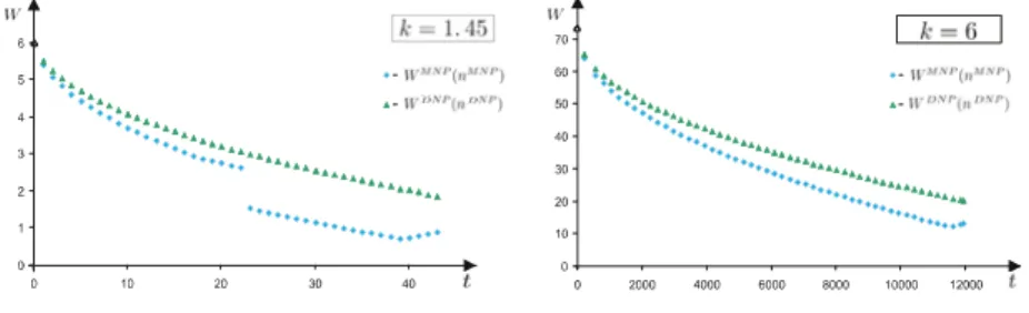
Figure 8 exemplifies the results of our simulations, when θ = 2 and F = 0.2. The first plot shows that for k low and high t the free entry number of firms is larger under DN P . However, the previous result only holds at a small region in the parameters’ space. For higher k or/and smaller t the long run equilibrium number of firms is larger under M N P .
Figure 8: Free entry long-run number of firms.
Our results also emphasize the fact that there exists excess entry under both pricing policies, as nS is always lower than nM N P and nDN P. In addition, the excess entry distortion is lower for low t (see Figure 8).
As expected, the free entry number of firms is decreasing with F and increasing with θ, under both pricing policies.
3 8Notice that the second solution that may appear with M N P has nDN P is equal to nM N P. This only occurs when k
4.2
Welfare
We reach always higher free entry long-run aggregate total surplus with DN P , although for low t, WDN P(nDN P) is very close to WM N P(nM N P). When t rises, the difference between these welfare levels increases (see for instance when θ = 2 and F = 0.2 at Figure 9). As in the standard Hotelling model, for both pricing policies welfare decreases when t rises.
5
Conclusion
The issue of whether price discrimination should be prohibited has been previously addressed in a setup where consumer differ according to one observable characteristic (location). Under this setup mill linear pricing and delivered linear pricing have been compared and it has been shown that, if there’s spatial contestability (firms can costless relocate), then in the long-run delivered linear pricing yields higher welfare, and, consequently, discriminatory prices should be allowed.
This paper considers a model where consumers simultaneously differ according to one unobservable (quality preferences) and one observable characteristic (location - brand preferences). In these circum-stances nonlinear prices arise in equilibrium. The main question addressed in this work is whether firms should be allowed to discriminate according to the observable characteristic. In other words, should firms be allowed to practise different nonlinear contracts at each location or should they be forced to set an unique nonlinear contract?
We showed that, when firms can costless relocate and set nonlinear contracts to screen consumers according to their preference for quality, delivered nonlinear pricing may bring smaller, equal or higher free entry equilibrium number of firms than mill nonlinear pricing, depending on the degree of asymmetric information and the degree of differentiation. The fact that the number of product varieties (free entry number of firms) may be higher under delivered nonlinear pricing is not present at Norman and Thisse (1996) and occurs when consumers types are more similar and differentiation is close to the level where local monopolies start to appear.
Our results corroborate Norman and Thisse (1996), under spatial contestability, in terms of too much product variety (excess of entry) with both mill nonlinear pricing and delivered nonlinear pricing since the free entry social optimal number of firms is always smaller than the free entry equilibrium number of firms when setting mill nonlinear pricing and delivered nonlinear pricing. This also happens in terms of welfare, since in the long-run delivered nonlinear pricing yields higher welfare than mill nonlinear pricing, thus, our results, support the view that discriminatory nonlinear prices should not be prohibited.
Besides extending previous results on the desirability of price discrimination according to some ob-servable characteristic, our work provides a comparison of mill nonlinear pricing and delivered nonlinear pricing which is interesting on its own as these two pricing policies have not been compared before.
Interesting extensions of our work would be to consider scenarios where we have a different proportion of types at each location or where brand preferences interact with quality preferences.
Appendix
A
Monopoly analysis
Consider a monopolist located at dm= 0. In this section we analyze the monopolist mill and delivered nonlinear contracts.
A.1
Mill nonlinear pricing
When the monopolist is not allowed to offer different nonlinear contracts at each location, his demand from type θ consumers is determined by the location, ˆdθm, where type θ is indifferent between buying from him or not buying at all:
θ ui− t ˆdθm− pi= 0 ⇔ ˆdθm=
θ ui− pi
t .
If the monopolist sells to both types of consumers, he will offer (¯pm, ¯um) and (pm, um) that solve the following problem: max ( ¯pm,¯um),(p m,um) µ ¯ pm− ¯ u2 m 2 ¶ ˆ d¯θm+ µ p m− u2 m 2 ¶ ˆ dθm subject to incentive compatibility constraints and feasibility constraints:
IC¯θ : ¯θ ¯um− ¯pm≥ ¯θum− pm ICθ : θ um− p
m≥ θ¯um− ¯pm
F C : 0 ≤ ˆdθm≤ 1 for θ = θ, θ
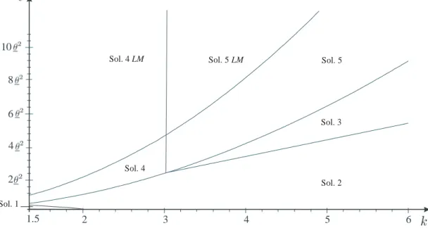
The Kuhn-Tucker conditions have multiple solutions39. Obviously, the solution of the monopolist problem is the one which yields the highest profit. Therefore, the optimal nonlinear contracts, which hold for different parameters sets, are given by:
Sol. 1 um= 2θ − ¯θ and pm= θ(2θ − ¯θ) − t ¯ um= ¯θ and ¯pm= ¯θ 2 + (θ − ¯θ)(2θ − ¯θ) − t Sol. 2 um= ¯θ and pm= ¯θ 2 − t Sol. 3 um= θ and pm= 3 4θ 2 ¯ um= ¯θ and ¯pm= ¯θ 2 − t Sol. 4 um= ¯θ and pm= 34¯θ 2 Sol. 5 um= θ and pm= 3 4θ 2 ¯ um= ¯θ and ¯pm=34¯θ 2
Incentive Compatibility Constraints are not binding, except at Sol. 1 (where IC¯θ binds). At Sol. 1, Sol. 2 and Sol. 3, the monopolist covers all the market for type ¯θ (that is, ˆd¯θ
m = 1). Notice that the quality offered by the monopolist to each type is the socially optimal, except for type θ at Sol. 1.
3 9We also achieved some undetermined solutions which could be represented by one of the stated solutions since the profits
from these possible but undetermined solutions are equal to the profits of other determined solutions and their intervals’ limits belong to the determined solutions intervals’ limits.


![Figure 3: Duopoly Delivered Nonlinear Pricing Contracts when t is High where: 2Reg ∗ C ([0, d C [) and C ¯θ ([d C , 1 2 ]) 3Reg ∗ I ([0, d[), Cˆ ([ ˆ d, d C [) and C ¯θ ([d C , 1 2 ]) 4Reg ∗ M ([0, d ∗ [), I [d ∗ , d[, Cˆ ([ ˆ d, d C [) and C θ ¯ ([d C , 1](https://thumb-eu.123doks.com/thumbv2/123dok_br/19221495.962933/13.892.173.742.309.534/figure-duopoly-delivered-nonlinear-pricing-contracts-high-reg.webp)