PHASE CHANGE MODELLING FOR NON-ISOTHERMAL
FLOWS: A MATHEMATICAL, NUMERICAL AND
COMPUTATIONAL MODEL FOR PURE SUBSTANCES
UNIVERSIDADE FEDERAL DE UBERLˆ
ANDIA
FACULDADE DE ENGENHARIA MECˆ
ANICA
PHASE CHANGE MODELLING FOR NON-ISOTHERMAL FLOWS: A
MATHEMATICAL, NUMERICAL AND COMPUTATIONAL MODEL
FOR PURE SUBSTANCES
Tese apresentada ao Programa de P´os-gradua¸c˜ao em Engenharia Mecˆanica da Universidade Federal de Uberlˆandia, como parte dos requisitos para a obten¸c˜ao do t´ıtulo de DOUTOR EM ENGENHARIA MECˆANICA.
´
Area de concentra¸c˜ao: Transferˆencia de Calor e Mecˆanica dos Fluidos.
Orientador: Prof. Dr. Aristeu da Silveira Neto
Dados Internacionais de Catalogação na Publicação (CIP) Sistema de Bibliotecas da UFU, MG, Brasil.
D812
2018 Duarte, Bernardo Alan de Freitas, Phase change modelling for non-isothermal flows [recurso eletrônico] : a mathematical, numerical and computational model for pure substances / Bernardo Alan de Freitas Duarte. - 2018.
Orientador: Aristeu da Silveira Neto.
Tese (Doutorado) - Universidade Federal de Uberlândia, Programa de Pós-Graduação em Engenharia Mecânica.
Modo de acesso: Internet.
Disponível em: http://dx.doi.org/10.14393/ufu.te.2018.795 Inclui bibliografia.
Inclui ilustrações.
1. Engenharia mecânica. 2. Escoamento bifásico - Modelos matemáticos. 3. Escoamento bifásico - Simulação por computador. I. Silveira Neto, Aristeu da, 1955- (Orient.) II. Universidade Federal de Uberlândia. Programa de Pós-Graduação em Engenharia Mecânica. III. Título.
2222 !"#$""%# &&'""&(%")&)"!*"'#&# %15+,-0'"&. 525 012345627874:47458;740<45;=1728
>??@ABCDEF?A?G@?H@DIDABGJKLM@DANDEF?BIOCHBCPD@QDRBSTCQSD
UVWX?F?YDVBKABZVQ[D\C]^_^_\`[?S?_R\aD[D^_^L`DQ@@?aDCbDRcCQSD\deB@[TCAQDLRM\>OGfghiiLji^ kB[Bl?CBmnfhof^fjLh^g^LpppWq?KH@DAWIBSDCQSDWNlNWe@LKBSq?KIBSrIBSDCQSDWNlNWe@
s45tu
8;01uw`B@CD@A?U[DCABx@BQbDKyND@bB t8s5z{0;8w__h^fOR>iif
|54874{u1{41s58}~uwk@DCKlB@CSQDAB>D[?@BRBSTCQSDA?Kx[NQA?K;21874460268wyQCTIQSDA?Kx[NQA?KBk@DCKlB@CSQDAB >D[?@
6 58708}~u4t41 418528t4{=12{8wYOydkUy
szs0;u78s464wGPDKBSPDCHBI?AB[[QCHl?@C?CLQK?bPB@ID[?pKmDIDbPBIDSD[\CNIB@QSD[DCAS?IqNbD?CD[I?AB[l?@qN@B KNeKbDCSBK
u5241s87u5wG@?lWy@WU@QKbBNADaQ[VBQ@DYBb?
UkBKBl?Q85u3878BI@BNCQF?qe[QSD\@BD[QDADC?DNAQbJ@Q?A?De?@DbJ@Q?ABRBSTCQSDA?Kx[NQA?K\`[?S?G\>DIqNKaDCbD RcCQSD\BI ijABDH?Kb?AB^i_g\KigP?@DK\S?IDKBHNQCbB`DCSDODIQCDA?@Dm
G@?lWy@WU@QKbBNADaQ[VBQ@DYBb?n?@QBCbDA?@oLdxd G@?lWy@Wa?[QAcCQ??A@QHNBKAB>D@VD[P?Ldxd G@?lWy@WU[ABIQ@UqD@BSQA?>DVD[[QCQXNCQ?@Ldxd y@WRQ[[BCDRD@CKQ[[D@D[BLdxd
G@?lWy@WMNBCbPB@>D@[?K@QBHB@xQ[P?LG?[QdaG y@WQSD@A?aB@lDbLGBb@?e@K
deB@[TCAQD\ijABDH?Kb?AB^i_g
y?SNIBCb?DKKQCDA?B[Bb@?CQSDIBCbBq?@88 ¡¢{ £ ¤¥¦¤¢\¢§¨¨¢© ª¢t «¨¬¢6¦¢\BIijig^i_g\K _mif\S?Cl?@IBP?@@Q??®SQD[AB`@DK¯[QD\S?IlNCADIBCb?C?D@bW°]\±_]\A?yBS@Bb?C]gWfj\ABgAB?NbNe@?AB^i_W
y?SNIBCb?DKKQCDA?B[Bb@?CQSDIBCbBq?@6¢¢¤¢5¢«¦¨{ £ ²¢\¢§¨¨¢© ª¢t «¨¬¢6¦¢\BIijig^i_g\K _mf°\S?Cl?@IBP?@@Q??®SQD[AB`@DK¯[QD\S?IlNCADIBCb?C?D@bW°]\±_]\A?yBS@Bb?C]gWfj\ABgAB?NbNe@?AB^i_W
y?SNIBCb?DKKQCDA?B[Bb@?CQSDIBCbBq?@ 041s45{85;u6³524 45:2;u\0¨¦´¢4µ¬¤¢\BIijig^i_g\K_°mh\S?Cl?@IB P?@@Q??®SQD[AB`@DK¯[QD\S?IlNCADIBCb?C?D@bW°]\±_]\A?yBS@Bb?C]gWfj\ABgAB?NbNe@?AB^i_W
y?SNIBCb?DKKQCDA?B[Bb@?CQSDIBCbBq?@8¨¬¦ 6£ 1¬¢\¢§¨¨¢© ª¢t «¨¬¢6¦¢\BI_iig^i_g\Ki¶mf°\ S?Cl?@IBP?@@Q??®SQD[AB`@DK¯[QD\S?IlNCADIBCb?C?D@bW°]\±_]\A?yBS@Bb?C]gWfj\ABgAB?NbNe@?AB^i_W
y?SNIBCb?DKKQCDA?B[Bb@?CQSDIBCbBq?@t¤ t ·¤¨3 3 \0¨¦´¢4µ¬¤¢\BI_iig^i_g\Kigmif\S?Cl?@IBP?@@Q? ?®SQD[AB`@DK¯[QD\S?IlNCADIBCb?C?D@bW°]\±_]\A?yBS@Bb?C]gWfj\ABgAB?NbNe@?AB^i_W
y?SNIBCb?DKKQCDA?B[Bb@?CQSDIBCbBq?@¡ ¢¨§ ¬¸\0¨¦´¢4µ¬¤¢\BI_iig^i_g\K_imfj\S?Cl?@IBP?@@Q??®SQD[AB `@DK¯[QD\S?IlNCADIBCb?C?D@bW°]\±_]\A?yBS@Bb?C]gWfj\ABgAB?NbNe@?AB^i_W
UDNbBCSQADABABKbBA?SNIBCb?q?ABKB@S?ClB@QADC?KQbBP¹qKmpppWKBQWNlNWe@KBQS?Cb@?[DA?@ºBbB@C?WqPq»
DSD?¼A?SNIBCb?ºS?ClB@Q@½QAº?@HD?ºDSBKK?ºBbB@C?¼i\QCl?@IDCA??SJAQH?VB@Q®SDA?@¾¿ÀÀÁ¿ÀB?SJAQH?>>4¿{48¾ÃW
First, I would like to thank God for allowing me to live great experiences in Uberlˆandia. I thank my supervisor, Prof. Dr. Aristeu da Silveira Neto, for the constant example of dedication and respect. For providing the support in the present work, I thank the Graduate Mechanical Engineering program, specially the Laboratory of Fluid Mechanics (MFLab) of UFU (Federal University of Uberlˆandia).
I would like to thank my family for the inconditional love. I thank my mother Iara for her sweetness, my father Jo˜ao for his trust and my sister Gisele for the complicity. I thank my fianc´e Pedro for teaching me that life has meaning only when we put love above all. In memory, I thank my mother-in-law Beatriz who taught me that a new day brings possibility to everything goes right.
I thank my friend H´elio Ribeiro Neto for being good and kind to me whenever I needed. For all the colleagues and staff from MFLab, I’m deeply gratefull for each moment lived. I’m also gratefull to my master degree supervisor, Hers´ılia de Andrade e Santos, who told me about the Graduate Mechanical Engineering program of UFU.
DUARTE, B.A.F., Phase change modelling for non-isothermal flows: A mathematical, numerical and computational model for pure substances. 2018. 178 f. Tese de Doutorado, Universidade Federal de Uberlˆandia, Uberlˆandia.
RESUMO
A dinˆamica de fluidos computacional ´e uma importante ferramenta para o estudo de es-coamentos presentes na natureza e em aplica¸c˜oes de engenharia. A modelagem computacional de problemas t´ıpicos de engenharia permite aumentar a eficiˆencia de processos produtivos e de equipamentos em diversos setores da economia. Al´em disso, o estudo de caracter´ısticas funda-mentais de escoamentos possibilita a cria¸c˜ao de um arcabou¸co te´orico importante para diversas linhas de pesquisa dessa ´area. Nos ´ultimos anos, a modelagem de problemas de mudan¸ca de fase tem sido conduzida utilizando modelos computacionais. Na presente tese de doutorado, foi desenvolvido um modelo matem´atico, num´erico e computacional de escoamentos n˜ao-isot´ermicos com mudan¸ca de fase. O c´odigo MFSim foi utilizado para a performance de todas as simula¸c˜oes computacionais e o cluster do Laborat´orio de Mecˆanica dos Fluidos (MFLab) foi empregado para a execu¸c˜ao das simula¸c˜oes na Universidade Federal de Uberlˆandia (UFU). O modelo computa-cional foi verificado e validado com in´umeros casos da literatura. Finalmente, um complexo caso de condensa¸c˜ao de contato direto (DCC) em cross-flow foi conduzido, demonstrando a potencial-idade do c´odigo MFSim para modelar at´e mesmo problemas de grande complexpotencial-idade. Problemas de ebuli¸c˜ao de l´ıquido ao redor de uma bolha de vapor foram utilizados para vallida¸c˜ao com solu¸c˜ao te´orica e anal´ıtica. Os resultados do presente trabalho apresentaram baixos desvios em rela¸c˜ao aos resultados pr´evios da literatura. Correntes esp´urias foram investigadas e quantificadas. Finalmente, for¸cas particulares a problemas de mudan¸ca de fase em CFD foram quantificadas e sua influˆencia nos problemas estudados foram nulas mesmo para situa¸c˜oes cr´ıticas.
ABSTRACT
The Computational Fluid Dynamic (CFD) is an important methodology to study the charac-teristics of flows in nature and in several engineering applications. Modelling non-isothermal flows may be usefull to predict the main flow dynamics which allows the improvement of efficiency in equipments and processes for industrial purpose. In addition, investigations using computational models may provide key information about the fundamental characteristics of flow, developing the theoretical groundwork of physical processes. In the last years, the topic of phase change has been intensively studied using CFD due to the computational and numerical advances reported in the literature. In the present work, phase change is studied using a mathematical, numerical and computational model developed in this thesis. The homemade code MFSim was used to run all the computational simulations in the cluster from the Fluid Mechanics laboratory (MFLab) from the Federal University of Uberlandia (UFU). The computational model was verified and validated against several cases from the literature. The model developed in the present thesis showed results with high accuracy and low differences compared to previous works in the literature. After the performance of several validation cases, some topics were deeply investigated. Finally, a com-plex case study of Direct contact condensation (DCC) was studied and the computational model provided accurate results compared to the literature. The present thesis reported the advances on modelling computationally the topic of phase change using the homemade code MFSim and several interesting conclusions were developed and some numerical issues were overcame. Boiling cases were validated against theoretical and analytical solution from the literature. The results show low deviations compared to the references. Finally, spurious currents magnitude were quan-tified for phase change problems and particular forces due to phase change were investigated. The results show null importance of these forces in the phase change model studied.
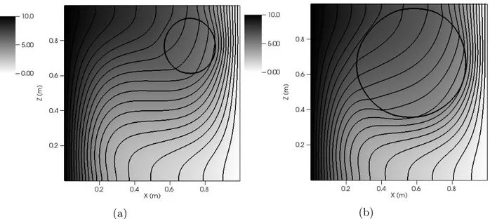
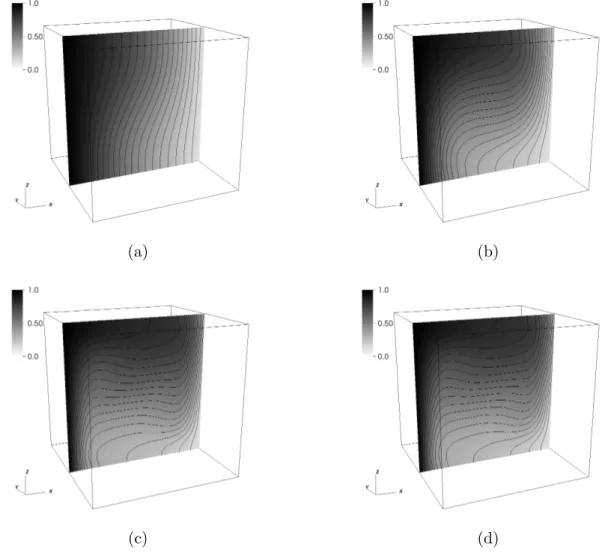
1.1 Central slice showing isotherms considering Pr=0.71 and Gr=1.4×10³(a), Gr=1.4× 10⁴ (b), Gr=1.4×10⁵ (c), Gr=1.4×10⁶ (d). . . . 5
1.2 Isotherms at central xz-plane for r = 0.15L (a) and r = 0.31L (b). Interface is represented by a contour line. . . 6
1.3 Velocity vectors at central xz-plane for A = 1.0 (a) andA = 0.33 (b). Interface is represented by a contour line. . . 6
1.4 Isotherms at central xz-plane for the case of thermal transfer increase (a) and reducement (b). Interface is represented by a contour line. . . 7
1.5 Tollmien–Schlichting instability in a case of single-phase flow natural convection. 8
1.6 Spurious currents in phase simulations considering m˙′
= 10.0 using a diffuse (a) and a sharp (b)interface treatment. . . 9
1.7 Interface and mesh configuration (a) at the initial time of the simulation and (b) at the final time. . . 9
1.8 Interface and mesh configuration (a) at the initial time of the simulation and (b) at the final time. . . 10
1.9 Water vapour bubble in condensation at the initial and final time of the compu-tational simulation. . . 10
1.10 Water vapour jet in cross-flow with liquid water. . . 11
4.1 Boiling liquid jet with an immersed conical surface at time t=0.17s (a) and t=1.37s (b). . . 39
4.2 Three-dimensional view of the general computational domain of the simulations performed in the present work. . . 40
5.1 Three-dimensional view of the u-velocity component field at 10.0s. . . 44
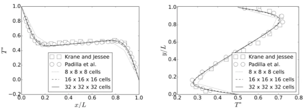
5.2 Dimesionless temperature along the line T∗
(x, L/2, L/2) and T∗
(L/2, y, L/2), respectively, for Ra= 1.89×10⁵ with OB . . . . 47
5.3 Dimensionless temperature along the line T∗
(x, L/2, L/2) and T∗
(L/2, y, L/2), respectively, for Ra= 1.89×10⁵ with NOB . . . . 48
5.4 Isotherms of the present study at central xz-plane for P r = 0.71 and: (a) Ra=1.0×10³; (b) Ra=1.0×10⁴; (c) Ra=1.0×10⁵ and (d) Ra=1.0×10⁶. . . 50
5.5 Isotherms of the Wan, Patnaik e Wei (2001) at central xz-plane for P r = 0.71
and: (a) Ra=1.0×10³; (b) Ra=1.0×10⁴; (c) Ra=1.0×10⁵ and (d) Ra=1.0×10⁶. 50
5.6 Isotherms from the present work with the isotherms at the central xz-plane for
P r= 0.71and: (a) Ra=1.0×10³; (b) Ra=1.0×10⁴; (c) Ra=1.0×10⁵ and (d)
Ra=1.0×10⁶. . . . 51
5.7 Isotherms at central xz-plane for r = 0.15L (a) and r = 0.31L (b). Interface is represented by a contour line. . . 53
5.8 Velocity field at the central xz-plane considering r = 0.15L (a) and r = 0.31L
(b). The interface is represented by a contour line. . . 53
5.9 Temperature and isotherms visualization for r = 0.15L (a) and r = 0.31L (b). The interface is represented by a contour line. . . 53
5.10 Frontal view of the central xz-plane with interface evolution using adaptive mesh at times 2.25s (a), 4.49s (b). . . 56
5.11 Frontal view of the central xz-plane with interface evolution using adaptive mesh at times 6.74s (a), 8.99s (b). . . 56
5.12 Frontal view of the central xz-plane with interface evolution using adaptive mesh at times 11.24s (a) and 13.48s (b). . . 57
5.13 Isotherms (a), velocity vectors (b) at time 13.48s. . . 58
5.14 Rayleigh-Taylor instability at 13.48s. . . 59
5.15 Interface evolution with adaptive mesh at times 9.05s (a), 18.09s (b) for A= 0.33. 59
5.16 Interface evolution with adaptive mesh at times 27.14s (a), 36.19s (b) forA= 0.33. 60
5.17 Interface evolution with adaptive mesh at times 45.24s (a) and 54.29s (b) for
5.18 Isotherms (a), velocity vectors (b) at time 54.29s. . . 61
5.19 Rayleigh-Taylor instability at 54.29s considering Atwood number of 0.33. . . 61
5.20 Velocity in centralxz-plane for Ra= 104 with OB (left) and NOB (right) . . . 63
5.21 Vorticity in central xz-plane forRa= 104 with OB (left) and NOB (right) . . . 64
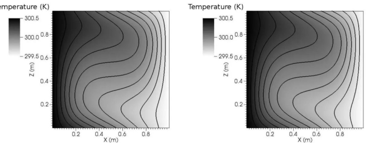
5.22 Temperature in centralxz-plane for Ra= 104 with OB (left) and NOB (right) . 65
5.23 Velocity in centralxz-plane for Ra= 106 with OB (left) and NOB (right) . . . 65
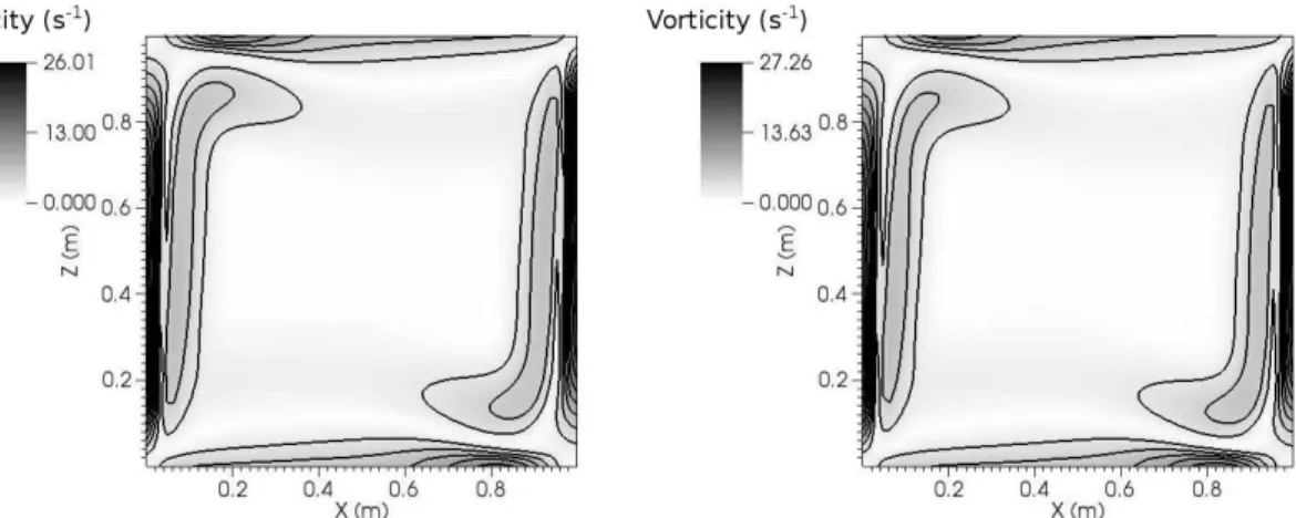
5.24 Vorticity in central xz-plane forRa= 106 with OB (left) and NOB (right) . . . 66
5.25 Temperature in centralxz-plane for Ra= 106 with OB (left) and NOB (right) . 67
5.26 Velocity in centralxz-plane for Ra= 108 with OB (left) and NOB (right) . . . 67
5.27 Vorticity in central xz-plane forRa= 108 with OB (left) and NOB (right) . . . 68
5.28 Temperature in centralxz-plane for Ra= 108 with OB (left) and NOB (right) . 69
5.29 Velocity in centralxz-plane for Ra= 1010 with OB (left) and NOB (right) . . . 69
5.30 Vorticity in central xz-plane forRa= 1010 with OB (left) and NOB (right) . . . 70
5.31 Temperature in centralxz-plane for Ra= 1010 with OB (left) and NOB (right) 70
5.32 Tollmien–Schlichting instabilities (left) and hairpin instabilities (right) . . . 71
5.33 Line segments used to evaluate theu, v and w velocity components . . . 74
5.34 u velocity component for the line segment AB in the central xz-plane with OB and NOB for Ra = 104 (upper left), Ra = 106 (upper right), Ra = 108 (lower
left) and Ra= 1010 (lower right). . . . 74
5.35 v velocity component along the line segment CD in the centralxz-plane with OB and NOB for Ra = 104 (upper left), Ra = 106 (upper right), Ra = 108 (lower
left) and Ra= 1010 (lower right). . . . 75
5.36 w velocity component along the line segment EF in the centralxz-plane with OB and NOB for Ra = 104 (upper left), Ra = 106 (upper right), Ra = 108 (lower
left) and Ra= 1010 (lower right). . . . 76
5.37 Isotherms at central xz-plane from the present paper forP r= 0.71and Gr=1.4× 10³ (a), Gr=1.4×10⁴ (b), Gr=1.4×10⁵(c), Gr=1.4×10⁶ (d) . . . . 78
5.38 Temperature field and isotherms for Gr = 1.4×10³ and P r = 0.71 (a) as well
5.39 Temperature field and isotherms at central xz-plane considering Gr=1.4 ×10³
and P r = 0.71 (a), P rove = 1.06 (b) and P rove = 1.51 (c). The isotherms are
represented in 20 thin isovalue contours, the thick contour represents the interface position and temperature field is presented in grayscale. . . 81
5.40 Spatial mean Nusselt number evolution in time for the single-phase case (P r = 0.71) and two-phase flows cases with P rove= 1.06 and P rove= 1.51. . . 82
5.41 Temperature field and isotherms at central xz-plane considering the single-phase case with Gr=1.4×10³ and P r = 0.71 (a) and the two-phase flow cases with
Gr=1.4 ×10³ and P r
ove = 1.06 with r = 0.31L (b) and r = 0.4L (c) The
isotherms are represented in 20 thin isovalue contours, the thick contour represents the interface position and temperature field is presented in grayscale. . . 83
5.42 Spatial mean Nusselt number evolution for the single-phase case (P r = 0.71), two-phase flow withr = 0.31L(P rove= 1.06) and two-phase flow withr = 0.40L
(P rove= 1.06) . . . 83
5.43 Temperature field and isotherms at central xz-plane for the single-phase case with Gr=1.4×10³ and P r= 0.71(a) and the two-phase flow cases with Gr=1.4×10³
and P rove = 1.51 (b) and P rove = 2.30 (c). The isotherms are represented in
20 thin isovalue contours, the thick contour represents the interface position and temperature field is presented in grayscale. . . 85
5.44 Spatial mean Nusselt number evolution for the single-phase case (P r = 0.71), two-phase flow withr = 0.31L(P rove= 1.51) and two-phase flow withr = 0.39L
(P rove= 2.30). . . 86
5.45 Temperature field and isotherms at central xz-plane for the single-phase case with Gr=1.4× 10⁴ and P r = 7.10 (a) and for the two-phase flow cases with
Gr=1.4×10⁴ and P r
ove = 6.30 (b) and P rove = 6.22 (c). The isotherms are
represented in 20 thin isovalue contours, the thick contour represents the interface position and temperature field is presented in grayscale. . . 88
5.47 Temperature field and isothers at central xz-plane for the single-phase case with Gr=1.4×10⁴ andP r = 7.10(a) and for the two-phase flow cases with Gr=1.4× 10⁴ and P r
ove = 6.22 with r = 0.31L (b) and P rove = 6.22 with r = 0.40L
(c). The isotherms are represented in 20 thin isovalue contours, the thick contour represents the interface position and temperature field is presented in grayscale. . 90
5.48 Spatial mean Nusselt number evolution for the single-phase case (P r= 7.1) and two-phase flows cases with P rove = 6.22considering r = 0.31Land r= 0.40L. 91
5.49 Temperature field and isotherms at central xz-plane for the single-phase case with Gr=1.4×10⁴ and P r = 7.10 (a) and for the two-phase flow cases with
Gr=1.4 × 10⁴ and P r
ove = 6.3 with r = 0.31L (b) and P rove = 5.5 with
r = 0.39L (c). The isotherms are represented in 20 thin isovalue contours, the thick contour represents the interface position and temperature field is presented in grayscale. . . 92
5.50 Spatial mean Nusselt number evolution for the single-phase case (P r= 7.1) and two-phase flows cases with a dispersed phase with radius of 0.31L (P rove= 6.3)
and 0.39L (P rove= 5.5). . . 93
5.51 Temperature field and isotherms at central xz-plane considering Gr=1.4× 10³
and Pr=0.71 for the two-phase flow cases with Gr=1.4×10³ and Pr=0.71 with
Ecdis= 5Eccon and Brdis= 5Brcon (a) andEccon = 2Ecdis andBrcon = 2Brdis
(b). The isotherms are represented in 20 thin isovalue contours, the thick contour represents the interface position and temperature field is presented in grayscale. . 95
5.52 Temporal spatial mean Nusselt number variation for the cases with similar Prandtl and Grashof numbers. . . 96
5.53 Temperature and isotherms at central xz-plane for the cases with Gr=1.4×10³
and Pr=0.71withBrdis = 5Brcon (a) andBrcon = 2Brdis(b). The isotherms are
represented in 20 thin isovalue contours, the thick contour represents the interface position and temperature field is presented in grayscale. . . 97
5.54 Spatial mean Nusselt number evolution for the single-phase case (P r= 0.71) and two-phase flows cases with Gr=1.4×10³, P r
5.55 Temperature field and isotherms at central xz-plane for the cases with Gr=1.4×10³
and Pr=0.71withEcdis= 2Eccon (a) andEccon = 5Ecdis(b). The isotherms are
represented in 20 thin isovalue contours, the thick contour represents the interface position and temperature field is presented in grayscale. . . 98
5.56 Spatial mean Nusselt number evolution for the single-phase case (P r = 0.71) and two-phase flows cases with for Gr=1.4×10³,P r
ove= 0.71. . . 98
5.57 Interface contour in the simulations using the Delta and GFM methods, respec-tively, at time t=0.5s, considering m˙′′
= 0.10kg/(m2s). . . . 100
5.58 Bubble radius evolution for m˙′′
= 0.10 kg/(m2s) using the Delta (a) and GFM
(b) methods. . . 100
5.59 Interface contour in the simulations using delta and GFM, respectively, at time t=0.5s, considering m˙ ′′
= 0.10 kg/(m2s). . . . 103
5.60 Interface, temperature field and mesh configuration at time 3.5 s at the central xz-plane. . . 104
5.61 Interface contour with the Delta method at initial time (a) and at 3.0s (b). . . . 105
5.62 Interface contour with the GFM method at initial time (a) and at 3.0s (b). . . . 106
5.63 Bubble radius evolution using the Delta method (a), and the GFM method (b). . 106
5.64 Slice of the centralxz-plane showing the interface and the mesh configuration for the Delta methods at time t=0s (a) and t=3.6s (b) , considering a variable mass density flux with Ja= 2.0. . . 107
5.65 Interface at time 12.0 s where the dotted line represents the mesh of32×32×64
cells, the dashed line is the mesh configuration of 64×64×128 cells, and the continuos line shows the grid with 128×128×256 cells. . . 109
5.66 Interface at the initial time of the simulation (a) and at the final time (b). . . . 110
5.67 Interface and mesh configuration (a) at the initial time of the simulation and (b) at the final time. . . 110
5.68 Evolution in time of the spatial mean Nusselt number in the film boiling simulation.112
5.70 Central xz-plane with the interface contour at the beggining (a) and at the end (b) of the simulations of a single water vapor bubble condensation. . . 113
5.71 Time history of the water vapor bubble diameter from the simulations from the present paper and the results from the literature. . . 114
5.72 Central xz-plane with the interface contour and mesh configuration at the time
0.00005s of the simulation of a single water vapor bubble condensation. . . 115
5.73 Spurious currents for m˙′′
= 0.1 kg/(m2s) at 0.001 s, (a) with Delta and (b) with
GFM. . . 116
5.74 Interface contour for m˙ ′′
= 0.1 kg/(m2s) at 0.001 s, (a) with Delta and (b) with
GFM at simulation’s final time. . . 117
5.75 Spurious currents for m˙′′
= 1.0 kg/(m2s) at 0.001 s, (a) with Delta and (b) with
GFM. . . 117
5.76 Interface contour for m˙ ′′
= 0.1 kg/(m2s) at 0.001 s, (a) with Delta and (b) with
GFM at simulation’s final time. . . 118
5.77 Spurious currents form˙′′
= 10.0kg/(m2s) at 0.001 s, (a) with Delta and (b) with
GFM. . . 118
5.78 Interface contour for m˙ ′′
= 0.1 kg/(m2s) at 0.001 s, (a) with Delta and (b) with
GFM at simulation’s final time. . . 119
5.79 Bubble radius evolution in phase change simulations with and without the recoil force effects using the Delta method. . . 122
5.80 Magnitude of the effects from the surface tension force compared to the recoil force using the Delta method. . . 122
5.81 Bubble radius evolution in the phase change simulations using delta for the non-divergent form with and without the extra force term. . . 124
5.82 Magnitude of the effects of the surface tension force compared to the additional force using the Delta method, for m˙′′
= 0.1. . . 125
5.83 Magnitude of the effects from the surface tension force compared to the additional force using the Delta method considering m˙′′
= 10.0. . . 126
5.85 Interface of the condensing jet at simulation time of 45s. . . 130
5.86 Interface contour of the jet at t=0s (a), t=0.005s (b), t=0.010s (c), t=0.015s (d).131
5.87 Mesh configuration and interface contour of the jet at t=0s (a), t=0.005s (b), t=0.010s (c), t=0.015s (d). . . 132
5.88 Jet centerline trajectory according to the results from the present work and from Clerx et al. . . 133
5.1 Grid configuration, error, refinement ratio, convergence ratio and order of conver-gence for temperature. . . 46
5.2 Average relative difference (ε) between OB and NOB from experimental data of Krane e Jessee (1983) . . . 48
5.3 Dimensionless temperature for NOB for x/L = 0.2, x/L = 0.5 and x/L = 0.8
from the line T∗
(x, L/2, L/2) . . . 49
5.4 Dimensionless temperature for OB for x/L = 0.2, x/L = 0.5 and x/L = 0.8
from the line T∗
(x, L/2, L/2) . . . 49
5.5 Spatial mean Nusselt number at the east wall for a range of Rayleigh numbers. . 51
5.6 Spatial mean Nusselt number at the east wall for two values of bubble’s initial radius. . . 54
5.7 Data used in the simulations of modelling a Rayleigh-Taylor instability in non-isothermal flows. . . 55
5.8 Mean Nusselt number (N u), differences between different mesh configurations(ψ)
and between the computed values using NOB and the experimental correlation of Cowan, Lovegrove e Quarini (1982) (ε)for Ra= 1010. . . . 63
5.9 Mean Nusselt number at the east wall and difference between the computed values and literature. . . 72
5.10 Minimum and maximum u,v and wvelocity components. . . 73
5.11 Summary of the thermal transfer rate results to compute the effects of the overall Prandtl number variation. . . 81
5.12 Summary of the thermal transfer rate results to compute the effects of the bubble size variation. . . 84
5.13 Summary of the thermal transfer rate results to compute the effects of the overall Prandtl number and bubble radius variation. . . 86
5.14 Summary of the thermal transfer rate results to compute the effects of the overall Prandtl number variation. . . 89
5.15 Summary of the thermal transfer rate results to compute the effects of the bubble size variation. . . 90
5.16 Summary of the thermal transfer rate results to compute the effects of the overall Prandtl number and the bubble radius variation. . . 94
5.17 Bubble radius error ε (%) form˙′′
= 0.10kg/(m2s) . . . . 101
5.18 Assessment of mesh configuration in the simulations with m˙ ′′
= 0.1kg/(m2s). . 102
5.19 Assessment of mesh configuration in the simulations of film boiling. . . 108
5.20 Assessment of mesh configuration in the simulations of film boiling. . . 111
5.21 Fluid properties employed in the simulations of a single water vapor bubble con-densation. . . 112
5.22 Spurious currents using different m˙′′
for Delta and GFM methods at 0.001 s. . . 120
5.23 Simulation time for Delta and GFM methods. . . 120
Abbreviations
A Atwood number
AMR Adaptive mesh refinement CFD Computational Fluid Dynamic CSF Continuum surface force method CFL Courant-Friedrich-Lewis condition DCC Direct Contact Condensation DHC Differentially heated cavity Delta Delta function method DOI Digital Object Identifier GFM Ghost Fluid method Gr Grashof number Ja Jakob number
LES Large eddy simulations
MFLab Fluid Mechanics Laboratory of UFU NOB Non-Oberbeck-Boussinesq approximation OB Oberbeck-Boussinesq approximation
PLIC Piecewise-linear interface calculation method Pr Prandtl number
Ra Rayleigh number
STP Standart temperature pressure UFU Federal University of Uberlandia VOF Volume of Fluid method
We Weber number
Subscript
Greek letters
α volumetric fraction
β volumetric expansion coefficient
Cp Specific heat capacity [J/kg]
ε relative error [%]
ρ specific mass [kg/m3]
µ dynamic viscosity [kg/ms]
η AMR efficiency [%]
k Thermal conductivity [W/mK]
κ interface curvature
L Latent heat [J/kg]
ψ indicator function (VOF)
δ Delta de Dirac
σ superficial tension coefficient
Mathematical operators
∂ gradient
∇ gradient
∇2 Laplacian
R
LIST OF FIGURES xiv
LIST OF TABLES xvi
LIST OF SYMBOLS xx
1 INTRODUCTION 1
1.1 Objectives . . . 2
1.1.1 General objective . . . 2
1.1.2 Specific objectives . . . 2
1.2 Justification . . . 3
1.3 Originality of the present thesis . . . 3
1.4 Highlights . . . 5
1.4.1 Grashof number influence in local thermal transfer rate . . . 5
1.4.2 Atwood number influence in the development of a Rayleigh-Taylor instability 6
1.4.3 Prandtl number influence in local thermal transfer rate . . . 7
1.4.4 Benchmark between Oberbeck-Boussinesq approximation (OB) X new temperature-dependent specific mass approach (NOB) . . . 7
1.4.5 Particular forces in phase change problems included in the computational model . . . 8
1.4.6 Evaluation of spurious currents in phase change problems . . . 8
1.4.7 Calculation of the adaptive mesh refinement efficiency in several problems 8
1.4.8 Film boiling simulations using AMR . . . 9
1.4.9 Simulation of a water bubble condensation . . . 10
1.4.10 Simulation of steam jet in condensation subjected to a liquid cross-flow . 11
1.5 Thesis organization . . . 11
2 BACKGROUND 13
2.1 Non-isothermal flows without phase change . . . 14
2.1.1 Specific mass variations due to temperature field . . . 14
2.1.2 Influence of relevant dimensionless numbers on non-isothermal flows . . . 16
2.1.3 Influence of bubbles on non-isothermal flows . . . 18
2.2 Non-isothermal flows with phase change . . . 19
2.2.1 Computational simulations of phase change . . . 20
2.2.2 Jump conditions in phase change simulations . . . 22
2.2.3 Particular forces in phase change problems . . . 22
2.2.4 Adaptive mesh refinement (AMR) in phase change problems . . . 24
2.2.5 Direct contact condensation . . . 24
3 MATHEMATICAL MODEL 27
3.1 Non-isothermal flows without phase change . . . 27
3.1.1 Formulation using the Oberbeck-Boussinesq approximation (OB) . . . . 27
3.1.2 Formulation using the new temperature-dependent specific mass approach (NOB) . . . 28
3.2 Non-isothermal flows with phase change . . . 29
3.2.1 Description of the general mathematical formulation . . . 30
3.2.2 Additional term in the non-divergent form of momentum equation . . . . 32
3.2.3 Turbulence model . . . 33
3.2.4 Interface location and transport . . . 33
4 NUMERICAL AND COMPUTATIONAL MODEL 35
4.1 Numerical model . . . 35
4.1.1 Phase change model . . . 35
4.1.2 Interface treatment for pressure . . . 36
5 RESULTS 41
5.1 Numerical verification of the thermal energy equation in the MFSim code . . . . 42
5.2 Validation of the thermal energy equation in the MFSim code . . . 46
5.2.1 Validation case 1: OB and NOB models . . . 46
5.2.2 Validation case 2: Simulations of natural convection in single-phase flows 49
5.2.3 Validation case 3: Simulations of natural convection in two-phase flows . 52
5.2.4 Validation case 4: Numerical simulations of a Rayleigh-Taylor instability . 54
5.3 Benchmark between Oberbeck-Boussinesq approximation (OB) and a new temperature-dependent specific mass approach (NOB) . . . 62
5.4 Influence of dimensionless parameters on non-isothermal single-phase flows with-out phase change . . . 77
5.4.1 Influence of the Grashof number on single-phase flows . . . 77
5.4.2 Influence of the Prandtl number on single-phase flows . . . 78
5.5 Influence of the Prandtl number on non-isothermal two-phase flows without phase change . . . 79
5.5.1 Simulations where the Prandtl number from the dispersed phase was higher than the Prandtl number from the continuos phase . . . 80
5.5.1.1 P rdis > P rcon and the effects of the overall Prandtl number
variation was computed . . . 80
5.5.1.2 P rdis > P rcon and the effects of the bubble size variation was
evaluated . . . 82
5.5.1.3 P rdis > P rcon and the effects of the bubble size and overall
Prandtl number variation were simultaneously analyzed . . . . 84
5.5.2 The Prandtl number from the dispersed phase was lower than the Prandtl number from the continuos phase . . . 87
5.5.2.1 P rdis < P rcon and the effects of the overall Prandtl number
variation was computed . . . 88
5.5.2.2 P rdis < P rcon and the effects of the bubble size variation was
5.5.2.3 P rdis < P rcon and the effects of the bubble size and overall
Prandtl number variation were simultaneously analyzed . . . . 91
5.5.3 Simulations where the Prandtl number from the dispersed phase was the same from the continuos phase . . . 94
5.5.3.1 Influence of the Brinkman number in two-phase flows without phase-change . . . 95
5.5.3.2 Influence of the Eckert number in two-phase flows without phase change . . . 96
5.6 Validation of the phase change model in the MFSim code . . . 99
5.6.1 Validation case 1: Boiling with a constant mass density flux . . . 99
5.6.2 Validation case 2: Boiling simulations with a variable mass density flux . 103
5.6.3 Validation case 3: Simulation of film boiling with Rayleigh–Taylor instability106
5.6.4 Validation case 4: An ascending condensing water vapor bubble in a sub-cooled water liquid . . . 112
5.7 Evaluation of the spurious currents in phase change problems . . . 115
5.8 Evaluation of particular forces in phase change problems . . . 120
5.8.1 Analysis of the recoil force in momentum equation . . . 121
5.8.2 Analysis of the additional force in momentum equation . . . 123
5.9 Case study of two-phase flow with phase change: Direct contact condensation jet with cross-flow . . . 126
5.9.1 Physical model . . . 127
5.9.2 Data and statistical analysis . . . 128
5.9.3 Computational results . . . 128
6 CONCLUSIONS 135
7 FUTURE WORKS 138
INTRODUCTION
These chapter describes the objectives, justification, originality, highlights and organiza-tion of the thesis. The objective subsecorganiza-tion describes the main and secondary objectives; the justification subsection presents the arguments supporting the thesis motivation; the highlights subsection shows the main topics investigated in the present work; finally, the organization sub-section describes the arrangement employed in the thesis composition.
The present work was focused on modelling mathematically, numerically and computa-tionally phase change in non-isothermal flows. The study was restricted to investigate flows considering pure substances and monocomponent fluids. The continuos hypothesis was adopted and the fluids were considered Newtonian.
According to the First Law of the Thermodynamic, the energy from a given system cannot be created or destroyed, since it can only be transformed from one form to another. There are several phenomena in nature and in engineering applications where one form of energy is converted to another, respecting the principle of total energy conservation.
When flow is subjected to phase change, its physical state is modified and the fluid prop-erties are modified where the phase transition occured. It’s imperative to study the phase change phenomenon since the phase change process may deeply modify the fluid properties in the region where phase transition occurs. Water, for example, at Standart Temperature Pressure (STP) con-dition, presents specific mass of approximately1000kg/m3 when is liquid; however, water vapour
presents specific mass of approximately1.5kg/m3 (POLING; PRAUSNITZ; O’CONNELL, 2001).
In addition, phase change may severely modify the temperature field affecting the flow dynamics of several phenoma. In the present thesis, the phase change phenomenon was studied from a mathemathical, numerical and computational model developed which was applied to the in house code MFSim.
1.1 Objectives
The present work aimed to achieve one general objective and seven specific objectives. These objectives were described in details in the following subsections.
1.1.1 General objective
The main objective of the present work was to develop a mathematical, numerical and computational model of non-isothermal two-phase flows subjected to phase change. The MFSim code was the plataform chosen to the computational implementation of the model developed in the present thesis, as well as the model verification and validation.
1.1.2 Specific objectives
The following objectives were defined for the present work:
1. Develop a bibliographic revision about the state of art of computational modelling non-isothermal two-phase flows and phase change;
2. Develop the thermal energy module in the MFSim code and perform verification and vali-dation cases;
4. Develop a mathematical, numerical and computational model of two-phase flows with phase change;
5. Include the phase change model in the MFSim code and perform validation cases;
6. Compose scientific papers and reports from the results obtanied in the present work;
7. Compose the thesis.
1.2 Justification
The present thesis was the first work focused on the study of non-isothermal flows with phase change in the research group from the Fluid Mechanics Laboratory (MFLab) in the Federal University of Uberlandia (UFU). MFLab research group has a strong insertion in mathematical, numerical and computational methodologies for general fluid mechanics problems and most part of its motivation has been research projects related to the brazilian industry. However, the influence of phase change process and temperature field variations have been generally not taken into consideration in the previous investigations conducted before the present thesis; since the purpose of the previous works were restricted to evaluate other variables of interest.
Recently, some research problems from MFLab projects have required the study of some complex phenomena where phase change is relevant to the fluid dynamics of flow. Then, the justification of the present thesis is the development of the initial steps of a new research line in the MFLab group where phase change is studied.
The main contributions from the present work was the development of a energy equation module as well as a phase change module in the MFSim code, allowing to study several important engineering applications.
1.3 Originality of the present thesis
1. Mathematical, numerical and computational methodologies of a temperature-dependent specific mass approach for non-isothermal flows;
2. Mathematical, numerical and computational methodologies for flows subjected to phase change;
3. Evaluation of the influence of dimensionless parameters in non-isothermal flows such as the Grashof, Prandtl, Nusselt and Jakob numbers.
Additional original contributions were obtanied according to the thesis progression in time, such as the following items:
1. Investigation of the recoil force in phase change problems;
2. Evaluation of a particular effect in phase change problems when using the non-divergent form of momentum equation;
3. Computation of adaptive mesh refinement (AMR) efficiency in phase change simulations using MFSim code
4. Comparison between two different approaches of pressure interface treatment in phase change problems.
The introduction of a phase change model in the MFSim code was itself an original con-tribution in the brazilian research scenario, since few relevant publications from Brazil of flows with pure substances subjected to phase change have been found in the main cientific databases (ISI Web of Knowlegde and ScienceDirect).
1.4 Highlights
In this section, some results-oriented points were presented to provide the readers an overview of the main findings of the present thesis.
1.4.1 Grashof number influence in local thermal transfer rate
In single-phase flows, the increase of Grashof number increases the local thermal transfer rate and isotherms pattern. Figure 1.1 illustrates the isotherms for different Grashof numbers in a simulation of natural convection of single-phase flow.
(a) (b)
(c) (d)
Figure 1.1: Central slice showing isotherms considering Pr=0.71 and Gr=1.4 × 10³ (a), Gr=1.4×10⁴ (b), Gr=1.4×10⁵ (c), Gr=1.4×10⁶ (d).
(a) (b)
Figure 1.2: Isotherms at central xz-plane for r = 0.15L (a) and r = 0.31L (b). Interface is represented by a contour line.
1.4.2 Atwood number influence in the development of a Rayleigh-Taylor instability
The increase of Atwood number increases the intensity of the baroclinic torque and the speed of the developement of the Rayleigh-Taylor instability. In addition, the simulation with higher Atwood number presented a higher local thermal transfer rate. Figure 1.3 shows the velocity field for the simulations of Rayleigh-Taylor instability for Atwood number of 1 and 0.33, respectively.
(a) (b)
1.4.3 Prandtl number influence in local thermal transfer rate
In two-phase flows, the introduction of a dispersed phase with different Prandtl number than the continuos phase may affect the local thermal transfer rate. The inclusion of a dispersed phase with lower Prandlt number than the continuos phase would reduce the local thermal transfer rate; as well as, the inclusion of a dispersed phase with a higher Prandtl number than the continuos phase would increase the local thermal transfer rate.
Figure 1.4 shows the isotherms for the case where the inclusion of a dispersed phase have increased and reduced the local thermal transfer rate, respectively.
(a) (b)
Figure 1.4: Isotherms at central xz-plane for the case of thermal transfer increase (a) and reducement (b). Interface is represented by a contour line.
1.4.4 Benchmark between Oberbeck-Boussinesq approximation (OB) X new temperature-dependent specific mass approach (NOB)
(a)
(b)
Figure 1.5: Tollmien–Schlichting instability in a case of single-phase flow natural convection.
1.4.5 Particular forces in phase change problems included in the computational model The present work has described for the first time in the literature the importance of an additional force due to the use of the non-divergent form of momentum equation when phase change occurs. The magnitude of the force was quantified and its importance was evaluated in some test cases.
In additional, the recoil force was investigated. The recoil force effects were also measured in phase change simulations and its magnitude was compared to the effects of interfacial tension force.
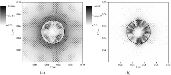
1.4.6 Evaluation of spurious currents in phase change problems
A diffuse and a sharp interface treatment for pressure were evaluated in phase change problems.
Figure 1.6 shows the spurious currents in phase change simulations considering a constant mass density flux of 10.0kg/m2s.
1.4.7 Calculation of the adaptive mesh refinement efficiency in several problems
(a) (b)
Figure 1.6: Spurious currents in phase simulations considering ˙m′
= 10.0 using a diffuse (a) and a sharp (b)interface treatment.
simulation of a Rayleigh-Taylor instability.
(a) (b)
Figure 1.7: Interface and mesh configuration (a) at the initial time of the simulation and (b) at the final time.
1.4.8 Film boiling simulations using AMR
(a) (b)
Figure 1.8: Interface and mesh configuration (a) at the initial time of the simulation and (b) at the final time.
1.4.9 Simulation of a water bubble condensation
Simulations of an ascending water bubble in condensation were performed and the results were compared to the literature. The figure below shows the water bubble interface at the initial time and after 3ms when condensation has almost completely vanished the vapor phase.
(a) (b)
1.4.10 Simulation of steam jet in condensation subjected to a liquid cross-flow
Simulations of a steam jet condensation with a liquid cross-flow was investigated. The figure below shows the interface contour from the saturated vapour jet in cross-flow with liquid water.
Figure 1.10: Water vapour jet in cross-flow with liquid water.
1.5 Thesis organization
The present work was organized in 7 chapters, namely:
❼ Chapter 1: it contains the introduction of the work. The objectives and the main
orig-inal contributions are described. The thesis main results are highlighted and the thesis organization is informed;
❼ Chapter 2: a background of the thesis topic is presented and the state-of-art of
❼ Chapter 3: the mathematical model used in the simulations is described. First, the
mathe-matical model of non-isothermal flows without phase change is presented; then, the math-emathical model of non-isothermal flows subjected to phase change is reported. Finally, a detailed subsection described the equations used in the cases where the specific mass variations were modelled according to the temperature field.
❼ Chapter 4: the numerical and computational models employed in the present work are
described. Details about the numerical discretizations, numerical treatment of interface and fluid variables were presented. The code MFSim is presented and its main characteristics are described.
❼ Chapter 5: the results are presented and compared to literature previous results. In addition,
the main results were summarized and a discussion was subsequentely provided.
❼ Chapter 6: the conclusions of the present thesis were presented. Each specific objective
previously defined in the thesis plan provided one or more conclusions according to the results obtanied.
❼ Chapter 7: it presents the main suggestions of future works based on the advances achieved
BACKGROUND
In this chapter, the authors present the central aspects related to modelling computationally non-isothermal flows with and without phase change, according to the literature. The main topics related to the thesis investigations are here described using the information found in the literature. The majority of ordinary fluid dynamic problems usually does not require information about the temperature field (TRYGGVASON; SCARDOVELLI; ZALESKI, ), since the variables of in-terest are usually the velocity or pressure (DUARTE et al., 2018). However, for most of the engineering applications, the temperature is an indispensable variable, affecting directly the flow characteristics such as in phase change problems (TANGUYet al., 2014) or indirectly, modifying the physical properties of fluids due to the temperature variations (MONTIEL-GONZALEZet al., 2015; DUARTEet al., 2018).
The importance of the temperature field in the computational fluid dynamics (CFD) is usually restricted to problems where the effects of temperature are proeminent or necessary to the flow characteristics since it represents the additional costs to solve the energy equation (TRYGGVASON; SCARDOVELLI; ZALESKI, ). To model the phase change phenomenon, the temperature field is obviously necessary to be known in the computational simulations; however, for several other problems, the temperature field hardly call attention to the literature, although it may bring severe consequences to the flow dynamic (DUARTE et al., 2018).
compu-tational aspects of modelling non-isothermal flows without phase change are reported. Then, the state-of-art of modelling phase change computationally is presented and its main characteristics are described.
2.1 Non-isothermal flows without phase change
In this section, some topics related to the computational aspects of modelling non-isothermal flows without phase change are reported. First, the importance of the specific mass variations due to the temperature field will be described. Then, the influence of some dimensionless parameters in non-isothermal flows are presented. Finally, the influence of bubbles in non-isothermal flows are briefly reported.
2.1.1 Specific mass variations due to temperature field
Although the term “density” is more commonly used than “specific mass” in the literature, the authors of the present work consider that “density” is suitable for referring to the property of an object or of a composed substance. On the other hand, “specific mass” refers to the property of a substance. Therefore, in the present thesis, the term “specific mass” will be used to define the amount of mass per unit volume.
Most of the fluid physical properties are temperature-dependent since the variations of tem-perature may modify the fundamental characteristics of fluids (POLING; PRAUSNITZ; O’CONNELL, 2001). In the computational fluid dynamics (CFD), the importance of these fluids properties vari-ation is restricted to problems where the temperature fields affects directly the flow dyamics such as natural convection problems (MONTIEL-GONZALEZ et al., 2015). For most of the natural convection problems, the traditional Oberbeck-Boussinesq approximation is sufficient to model computationally the flow dynamic correctly. On the other hand, the majority of the engineering applications are related to turbulent flows and usually with the presence of strong temperature gradients (AKHTAR; KLEIS, 2013).
equa-tions. The later way requires to solve the flow as compressible, where the continuity equation is solved without the usual simplification seen for incompressible flows. The literature also presents another form to account the effects of specific mass variations without invoking OB or solving the diferential equations considering the flow as compressible. The later form is generally known as non-Oberbeck Boussinesq models (NOB), where the specific mass is considered variable in all the terms from the momentum and energy equations; although the continuity equation preserves the incompressible condition with null velocity-divergence.
The NOB method was fundamentally based on Markatos e Pericleous (1984), who previ-ously studied natural convection in a 2D numerical model. Markatos e Pericleous (1984) employed an extension of OB, considering specific mass as a function of the temperature in all the terms of the momentum and energy equations. More recently, Montiel-Gonzalez et al. (2015) presented a numerical investigation of thermal convection problems with a comparison between OB and a new temperature-dependent method for all the fluid properties, and considering null velocity divergence. Their work obtained numerical results with higher accuracy in the approach using variable fluid properties as functions of temperature.
Most of what is known about natural convection is due to the use of OB (GRAY; GIOR-DINI, 1976) and more than one hundred years after the publication of OB, it is still probably the most employed formulation for natural convection (ZEYTOUNIAN, 2003). Some of the lit-erature, e.g., Montiel-Gonzalez et al. (2015) and Markatos e Pericleous (1984), have proposed alternative mathematical formulations to achieve more accurate results about thermal transfer without invoking OB, but still assuming null velocity divergence. A large number of flows sub-jected to thermal transfer are assumed to be incompressible, since the impact of a variable specific mass in the continuity equation is not relevant. On the other hand, the effects of a temperature-dependent approach for the specific mass in the momentum equation are particularly important for non-isothermal flows, as previously stated by OB (BOUSSINESQ, 1903). Therefore, when the flow is assumed incompressible, the velocity divergence is small enough to be considered null. However, variations of the specific mass in the momentum and energy equations may be pertinent due to the influence of temperature on the properties of the fluid, as found by Montiel-Gonzalez et al. (2015).
temperature field is recently being more investigated in several non-isothermal problems and this research has been important for bringing new insights into thermal transfer mechanisms. Several studies have investigated the thermodependency of the fluid variables in non-isothermal flows, such as Darbouli et al. (2016) and Montiel-Gonzalez et al. (2015).
The relevance of the specific mass variations due to the temperature field is particularly critical to a major part of fluid dynamic problems, namely natural convection cases. The variations of specific mass plays an important role on the flow characteristics modifying the velocity and pressure fields. Therefore, the specific mass is modeled here using a temperature-dependent approach and a benchmark is conducted with the traditional Oberbeck–Boussinesq approximation (OB).
In the literature, similar numerical studies on non-Oberbeck–Boussinesq buoyancy induced flows have been reported in the laminar and turbulent regimes; however, no similar investigation has been presented in three dimensions, which is particularly relevant for turbulence.
2.1.2 Influence of relevant dimensionless numbers on non-isothermal flows
There are several dimensionless numbers related to the physics of non-isothermal flows such as the Grashof, Prandtl, Rayleigh, Eckert, Brinkman and Nusselt numbers. These dimensionless numbers generally characterize the relation between the temperature field and the flow dynamics. Next, these dimensionless numbers are briefly described.
The Grashof number represents the ratio of gravitational to viscous force on a fluid and it’s defined according to the following equation (WHITE, 1974):
Gr= gβ(Ts−T∞)L 3
ν2 (2.1)
where: g is the gravity acceleration field,β is the volumetric expansion coefficient, Ts is the
tem-perature at a given reference surface, T∞ is the temperature of reference, L is the characteristic
length andν is the kinematic fluid viscosity. The Prandtl number defines the ratio of momentum diffusivity to thermal diffusivity and it’s given by the following expression (WHITE, 1974):
P r= µCp
where: Cp is the specific thermal energy, µ is the dynamic viscosity and k is the thermal con-ductivity. The Rayleigh number consist of the product of Prandtl and Grashof numbers which is expressed below:
Ra=P rGr (2.3)
The Rayleigh number expresses the ratio between the buoyancy and viscosity forces as well as the ratio between the momentum and thermal difussivities. The Eckert number consist of the ratio between the kinetic energy by the boundary layer enthalpy and is defined by the expression given below:
Ec= u 2
CpδT (2.4)
where u is the local flow velocity, Cp is the specific thermal energy and δT is the difference between wall and local temperature. The Brinkman number is a dimensionless number associated to the ratio between the thermal energy produced by viscous transformation and thermal energy transported by molecular diffusion. The Brinkman number is given by the following expression:
Br = µu 2
k(Tw −T0)
(2.5)
where Tw is the wall temperature and T0 is the temperature of reference.
The Nusselt number may be defined according to the following expression (DEEN; KUIPERS, 2013):
N u= L ∆T
∂T
∂x|x=0 (2.6)
According to the literature, the Grashof and the Prandtl numbers directly affect the thermal transfer rate in non-isothermal flows. The work from Chandra e Chhabra (2012) investigated the impact of the variations of these dimensionless numbers on the Nusselt number and the later authors found the increasement of the Nusselt number when Prandtl and Grashof number increased. However. the later work studied only single-phase flows. The influence of the Grashof number on the Nusselt number is already consolidated in the literature (PADILLA; LOURENCO; SILVEIRA-NETO, 2013; WAN; PATNAIK; WEI, 2001) and its increasement necessarly increases the thermal transfer rate. However, the role of the Prandtl number is yet not so studied in the literature.
2.1.3 Influence of bubbles on non-isothermal flows
It has been extensively reported in the literature the increasement of the thermal transfer rate due to the introduction of bubbles in single-phase flows; however, this topic has not yet been completely elucidated.
The thermodynamic effects of the addition of bubbles in single-phase flows are widely described in several experimental and numerical studies in the literature. According to Deen e Kuipers (2013), it is generally agreed in the literature that the introduction of a gas into a liquid enhances the turbulence in the medium and thus increases the thermal transfer rate to immersed surfaces. Deen e Kuipers (2013) additionally defend that higher gas velocities enhances even more the thermal transfer rate. Deckwer (1980) suggested that the presence of bubbles can increase the thermal transfer rate in a gas-liquid bubble column by more than one order of magnitude. Oresta
(considering 3% of volume fraction).
According to Dabiri e Tryggvason (2015), the presence of moving bubbles generally in-creases the local thermal transfer. Bukhari e Siddiqui (2007) studied natural convection for two-phase flow and concluded that thermodynamic patterns, such as the thermal exchange at the interface, may be directly affected by some hydraulic patterns such as the velocity field. The authors from the later work concluded that the turbulent structures on the air and water phases played an important role enhancing the thermal and mass transfer rates. Chandra e Chhabra (2012) presented a quantitative analysis of the influence of the Prandtl and the Grashof numbers in single-phase flows, reporting the Prandtl number importance in regulating the thermal transfer rate on immersed surfaces in single-phase flows.
Although the literature has obtained, majority, higher thermal transfer coefficients in two-phase flows compared to single-two-phase flows; there is no quantitative analysis or conclusions elucidating the causes of the numerical or experimental results obtained. In addition, some works have presented opposite results, such as Qiu, Wang e Jiang (2014) which obtanined the decreasement of the thermal transfer rate by the inclusion of bubbles in the flow.
It’s imperative to examine the thermal transfer characteristics using dimensionless parame-ters in order to establish general conclusions and to improve the understanding of the underlying mechanisms involving the thermal transfer mechanisms. Since information about the thermal transfer rate in single-phase and two-phase flows are crucial to several industrial processes as well as in a variety of equipments employed in engineering applications, computational investigations may guide and improve the efficiency of the thermal transfer processes. In addition, new studies on these topics may report new insights into the thermal transfer mechanisms, openning new research opportunities related to non-isothermal two-phase flows.
2.2 Non-isothermal flows with phase change
2011).
The main topics related to the thesis investigations are reported in this section and the state-of-art of modelling phase change computationally are described according to the literature.
2.2.1 Computational simulations of phase change
Phase change is a relevant issue in industrial applications (HAELSSIG; THIBAULT; ETEMAD, 2010) since it plays a critical role in a large number of processes (WELCH; WILSON, 2000; JU-RIC; TRYGGVASON, 1998). Boiling, for example, is a highly efficient way to transfer thermal energy, notably in industrial thermal exchangers (NIKOLAYEV et al., 2016). Moreover, chemical separation techniques, such as distillation, are characterized by simultaneous mass and energy transfer (HAELSSIG; THIBAULT; ETEMAD, 2010). Droplet evaporation is another indubitable important phenomenon presenting great importance for certain applications (STROTOS et al., 2011), particularly burning liquid-fuels. The earlies phase change numerical works in the litera-ture presented important aspects of mathematical and numerical modelling which can be seen in (JURIC; TRYGGVASON, 1998) and (WELCH; WILSON, 2000). Later, several advances in mathematical and numerical modelling have been achieved and reported in the literature with even complex simulations for industrial applications (TANGUY et al., 2014).
Numerical simulations of phase change are relevant to collect information about flow char-acteristics since experiments dealing with phase change are usually difficult to be correctly con-ducted (PAN; WEIBEL; GARIMELLA, 2016) due to the small spatial scales (WELCH; WILSON, 2000) and the rapidity of phase change process (JURIC; TRYGGVASON, 1998). Phase change simulations present several numerical obstacles (TRYGGVASON; LU, 2015). One of the most challenging aspects is notably the physical properties discontinuities occuring at the interface between two fluids (TSUI et al., 2014). In addition, the jump conditions across the interface of fluid properties, such as pressure, represent an important aspect to be considered in phase change simulations (TANGUY et al., 2014).
interface treatment generally presents a poor representation of the jump conditions at the interface since the fluid properties are smoothed across the boundary between the two fluids (TANGUYet
al., 2014). The development of spurious currents at the interface is a typical consequence in the velocity field due to the employment of a diffuse interface treatment for pressure.
Fictitious velocities emerges due to an erroneous estimation of the surface tension force (HARVIE; DAVIDSON; RUDMAN, 2006) and pressure gradient according to the numerical schemes employed (AKHTAR; KLEIS, 2013). In addition, the spurious currents tend to be in-tensified in the phase change problems (TANGUY et al., 2014), then they should be particularly controlled in these numerical simulations. The spurious currents generally appear close to the interface when computations of a static bubble or droplet are performed with a diffuse interface treatment for pressure due to the surface tension force calculation (FRANCOIS et al., 2006). According to Tanguy et al. (2014), the spurious currents intensity increases when phase change occurs due to the jump condition on the velocity field. In addition, the presence of spurious cur-rents may be partly responsible for an inaccurate interface evolution in time since this boundary’s advection is performed using the local velocity field.
Tanguy et al. (2014) have presented inaccurate results for a diffuse interface treatment in phase change simulations. Other works in the literature using a diffuse interface treatment, as Samkhaniani e Ansari (2016) and Lee, R. e Aute (2017) found numerical results with a low deviation with the literature. More studies are necessary to understand the consequences of using a diffuse interface treatment instead of a sharp strategy for one or more fluid variables in phase change simulations. In addition, it’s appropriate to quantify these fictitious velocity field in the phase change simulations in order to evaluate its consequences and to visualize the behavior of the interface motion in time to confirm the acuracy of the numerical model employed.
following expression:
Ja= ρlCpl(T∞−Tsat)
ρvL
(2.7)
where: T∞ is the temperature of reference far from the dispersed phase, Tsat is the saturation
temperature and Lis the latent energy.
2.2.2 Jump conditions in phase change simulations
Literature presents two numerical strategies to impose jump conditions of fluid variables across the interface, namely the Whole Domain formulation and the Jump Condition formulation (TANGUYet al., 2014). The Whole Domain methodology uses a Delta Functions method (Delta), in which the jump conditions are smoothed around the interface, smearing out discontinuities terms. On the other hand, the Jump Condition formulation uses a Ghost Fluid Method (GFM) in which the interface is treated imposing the jump conditions by ghost cells (TANGUY et al., 2014; TANGUY; MENARD; BERLEMONT, 2007).
The Delta method computes the surface tension force using a continuum surface force (CSF) model (BRACKBILL; KOTHE; ZEMACH, 1992) which usually generates spurious currents due to a numerical imbalance between the pressure gradient and the related surface tension force (FRANCOIS et al., 2006). Even though the presence of spurious currents has been extensively observed by researchers since CSF conception, to date there has been little quantitative analysis of their importance (HARVIE; DAVIDSON; RUDMAN, 2006), specially when applied to problems involving phase change. Numerous approaches have been proposed to supress spurious currents; although, several methods have difficulties to not induce unphysical flows due to the numerical error in estimating the interfacial surface tension (PAN; WEIBEL; GARIMELLA, 2016). Con-versely, the GFM approach computes the surface tension force without a smooth transition due to a sharp jump condition for pressure at the interface (FRANCOIS et al., 2006).
2.2.3 Particular forces in phase change problems
additional force due to the use of the non-divergent form of momentum equation. For the first time in the literature of phase change, the additional force due to the use of the non-divergent form of momentum equation is presented and quantified. The need of this additional term in phase change problems is reserved to the use of the non-divergent form of momentum equation and the occurence of mass transfer at the interface. Since the interface cells do not present null-divergence velocity in phase change problems, the non-divergent form of momentum equation naturally receives an additional term from the continuity equation. The details of this extra force term are described in the mathematical model section; later, the computational results section presents a quantitative analysis of the additional force term in phase change simulations.
During phase change, a recoil force appears at the interface between the two fluids due to volume change (RAGHUPATHI; KANDLIKAR, 2016). The intensity of recoil force depends on the mass density flux occuring at the interface. The recoil force may be defined according to the following expression (NIKOLAYEV et al., 2016):
~
frecoil = ˙m′′
2 1
ρv −
1
ρl
~n (2.8)
where: m˙′′
is the mass density flux (this term is described in the mathematical model section),ρ
is the specific mass and~n is the normal vector.
compute the magnitude of this force and its importance to phase change problems.
2.2.4 Adaptive mesh refinement (AMR) in phase change problems
It’s known that an accurate numerical solution of partial differential equations rely on the discretization on a computational grid with sufficiently high resolution. On the other hand, the simulations using uniform grids overly increase the computational costs due to a large domain region unnecessarly refined. A uniform and fine grid is generally associated with a high compu-tational cost which may limit the applicability of solving several complex problems of interest. Conversely, the AMR methodology is a computational tool allowing the definition of a criteria to guide a spatially non-uniform mesh refinement according to an indicator function, such as vorticity, temperature gradient or interface presence.
AMR may provide a strategy to solve complex problems using lower computational re-sources compared to uniform grids (AKHTAR; KLEIS, 2013) and it reduces the computational power requirement without affecting the precision from the numerical results (NINGEGOWDA; PREMACHANDRAN, 2014). The interest in using AMR in multiphase flows is particularly large since the interface region frequently requires fine grids due to the calculation of high gradients and the rest of the domain usually do not require fine grids (NIKOLOPOULOS; THEODORAKAKOS; BERGELES, 2007).
Recently, phase change literature present several works which employ AMR strategy to model some large scale or complex problems. In the present work the refinement criteria was related to the interface location which the majority of works in the phase change literature does, such as Akhtar e Kleis (2013). In order to compute a quantitative evaluation of the improvement of time and computational power saved with AMR compared to uniform grids, an expression of AMR efficiency is used to quantify the enhancement of AMR strategy from the literature.
2.2.5 Direct contact condensation