Abstract
In this study, the discrete-time Volterra series are used to update parameters in a nonlinear finite element model. The main idea of the Volterra series is to describe the discrete-time output of a nonlinear system using multidimensional convolutions between the Volterra kernels represented in a Kautz orthogonal basis and the excitations. A metric based on the residue between the experimental and the numerical Volterra kernels is used to identify the parameters of the numerical model. First, the identification of the linear parameters is performed using a metric based only on the first order Volterra ker-nels. Then the nonlinear parameters are identified through a metric based on the higher-order kernels. The originality of this nonlinear updating method stems from the decoupling of linear and nonlinear parameters and the use of global nonlinear model. In order to put in light the applicability of this technique, this work focus on the iden-tification of the parameters in a nonlinear finite element model of a beam that was preloaded by compression mechanism. This work shows that the updated numerical model was able to represent the behaviour observed in the experimental measurements.
Keywords
Discrete-time Volterra series, Kautz filters, model updating, nonlin-ear finite element model, nonlinnonlin-ear identification, sensitivity.
Updating of a Nonlinear Finite Element Model
Using Discrete-Time Volterra Series
1 INTRODUCTION
In many cases, the dynamical behaviour is needed to design a mechanical system. Moreover, the knowledge of the dynamical behaviour of a structure is important to control its integrity and to
Philippe Bussetta a Sidney Bruce Shiki b Samuel da Silva c
a INEGI, Composite Materials and
Structures Research, Institute of Me-chanical Engineering and Industrial Management, Porto 4200-465, Portugal. [email protected]
b UFSCar - Federal University of São
Carlos, Mechanical Engineering Department, Rodovia Washington Luís, km 235, Zip Code: 13565-905, São Carlos, SP, Brasil. [email protected] cUniversidade Estadual Paulista - Unesp,
Faculdade de Engenharia de Ilha Solteira, Departamento de Engenharia Mecânica, Av. Brasil, 56, Zip Code: 15385-000, Ilha Solteira, SP, Brasil. [email protected]
http://dx.doi.org/10.1590/1679-78253853
predict its service life. In the practical systems, nonlinear effects due to large displacements, gaps, jumps, discontinuities, etc. are very common (e.g. Worden and Tomlinson (2001)). The nonlinear finite element method is a very powerful tool to study the nonlinear vibrations. Nevertheless, it is not easy to identify the parameters of the nonlinear model due to the uncertainties in the modelling of the experimental system (e.g. the mechanical properties, the boundary conditions). Despite of the important number of investigations, the nonlinear model updating techniques are not mature as the classical linear ones.
A bibliography review on the state of the art nonlinear system identification techniques in structure dynamics is presented by Noël and Kerschen (2017). Furthermore, a bibliography review of the nonlinear updating methods is exposed by Bussetta et al. (2017). Generally, the updating methods are based on the minimisation of an objective function or a metric that represents the difference between the numerical results and the experimental data. This objective function can use data in the frequency domain or in the time domain. The Volterra series can be used to defined this objective function (e.g. Wu and Kareem (2014); Guo et al. (2013)). In the paper of Shiki et al. (2012) the authors made a numerical comparison of a nonlinear model updating technique based on Volterra series and proper orthogonal decomposition. The last technique showed severe limitations, especially when considering higher levels of excitation of a model with lumped polynomial stiffness while the Volterra series showed a better performance with higher levels of nonlinearity. Generally speaking, the updating methods are applied by assuming linear models of the structure with lumped non-linearities, often assuming some kind of nonlinear springs as being the source of the nonlinear behaviour. Although this kind of model is able to reproduce the nonlinear phenomena (e.g. Kerschen et al. (2003)), it is actually a rough simplification of the structure.
1.1 Originality of this Work
The originality of this work stems from the updating of nonlinear finite element model of structures using the Volterra series, rather than using simplified linear elements with lumped nonlinearity. The dynamical behaviour of structure is modelled using nonlinear finite element model and experimental data are used to identify numerical parameters. These parameters are split in linear and nonlinear parameters. The value of the linear parameters is identified using linear error indicator which is computed with the linear response of Volterra series. The identification of nonlinear parameters is based on the full Volterra series.
1.2 Outline
This paper is organised in five sections. First, the experimental setup of a preloaded buckled beam is described (section 2). Then, the nonlinear finite element model is presented in the part 3. The section 4 deals with the model updating based on the Volterra kernels expanded in a Kautz orthogonal basis. Finally, some remarks are summarised (section 5).
2 EXPERIMENTAL SETUP
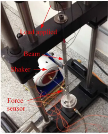
been the subject of experimental study to identify cubic stiffness non-linearity of single degree-of-freedom Duffing system Tang et al. (2015). The aim of this experimental setup is to study the vibra-tion of a preloaded beam. The test structure is composed of a vertical aluminium beam with dimen-sions of 460x18x2 mm (see figure 1). The bottom of the beam is clamped and a preload is applied on the top of the beam. The experimental setup has a screw in the top of the beam to apply an axial preload force. The preload was adjusted by trial and error until just before the buckling load of the beam Tang et al. (2015). This was done to obtain a stronger nonlinear effect since the linear stiffness is reduced by applying the preload Kovacic and Brennan (2011). The excitation of the beam is gen-erated by an electrodynamic shaker attached at 65 mm from the bottom of the beam. A load cell is placed between the shaker and the beam to record the exciting force with an acquisition board system. The oscillation of the beam is measured using the velocity captured by a laser vibrometer in the middle of the beam. The sampling frequency is equal to 1024 Hz and 4096 samples are recorded at each experimental test. In previous papers, Scussel and da Silva (2016) and Shiki et al. (2014a) have demonstrated the nonlinear regime of vibration of this test bed using stepped sine test, FRFs and time-frequency plots. More details can be obtained in these references.
(a) General view (b) Scheme
Figure 1: Experimental setup.
3 NONLINEAR FINITE ELEMENT MODEL
The model of the preloaded buckled beam uses the classical updated Lagrangian formulation of the 3D nonlinear finite element method. In each time step the displacement field is computed according to the momentum equation (see Wriggers (2008); Belytschko et al. (2014)):
Where is the displacement, ρ is the mass density, is the Cauchy stress tensor and is the specific body forces. The material is modelled as visco-elastic using the Kelvin-Voigt law, then the value of the stress is given by:
: (2)
where is the fourth-order tensor of the Hooke's law, the strain tensor, the deviatoric parts of the strain-rate tensor and the coefficient of viscosity. Note that the evolution of the Cauchy stress tensor, , is computed thanks to the Jaumann's objective time derivative. The mesh used in this model is composed of linear hexahedral elements. The displacement fields is computed at each node of the elements. The deviatoric part of the Cauchy stress is evaluated using a 2x2x2 Gauss quadrature scheme. To overcome the locking phenomenon, the pressure is considered constant over the element and computed only at a central quadrature point. This is a so called selective reduced integration. After integration of the weak form of the equation (1) over the mesh, the system of equations becomes:
,
, (3)
where is the mass matrix and and are the internal and external force vectors. is the stiffness matrix. The dynamical behaviour is computed thanks to the generalised- method proposed by Chung and Hulbert (1993). With this time integration scheme, the unknowns are computed at the time Δ due to the value at the time . The equilibrium equation is rewritten pondering inertia forces by the parameter , and internal and external forces by the parameter :
(4)
Moreover, the relations between the displacements, the velocities and the accelerations are:
Δt
(5)
γ γ (6)
Second order accuracy, unconditional stability and optimal numeric dissipation of high frequencies is obtained for:
ρ
ρ (7)
ρ
ρ (8)
ρ
ρ (10)
where ρ is approximately the percentage of numerical damping for the highest frequency of the structure.
4 MODEL UPDATING
Firstly, the test structure is submitted to a low level of amplitude force generated by the shaker in order to observe the linear response of the beam. Next, a larger amplitude force is used to study the nonlinear behaviour of the structure. The input used is a chirp signal sweeping up the frequency range from 20 to 50 Hz during the first half of the test (2 seconds). This frequency range comprises the first vibration mode which was considerably affected by the nonlinearity of the structure. During the second half of the test the shaker is turned off and the beam vibrates freely until it reaches the rest position. The low level of amplitude force and the high level one are respectively used to identify the first Volterra kernel and the higher-order Volterra kernels (i.e. the second and the third Volterra
kernels). Both input signals are used to update the 3D nonlinear finite element model. Finally, a middle level of amplitude force generated by the chirp input signal as well as a low, a middle and a high level of a 35 Hz sinusoidal input signal1 are used to show that essentially the output signal from the updated nonlinear finite element model and the experimental one are similar.
Figure 2 presents the scheme of the numerical model. This numerical model use the homemade code Metafor of the University of Liege (see the official website of Metafor 2017). Like the experi-mental results, the solution of the numerical model is computed to the time of 4 seconds. In absence of any indication, the value of the numerical parameters are the following ones. The time step is 1/1024 seconds, the percentage of numerical damping for the highest frequency, ρ , is 0.01. The mesh is composed of 9 600 hexahedral elements. The length, the width and the depth are respectively meshed with 300, 8 and 4 elements. The aluminium beam is modelled as visco-elastic material (Young's modulus: 58 GPa, Poisson's ratio: 0.33, density: 2 700 kg m-3, coefficient of viscosity: MPa s). Unfortunately, an important unknown of this numerical model is the boundary condition on the top of the beam. Since in the used experimental setup it is not possible to identify the value of the preloaded force, it is assumed that the boundary conditions on the top of the beam are modelled with an constant force, F, a linear spring – with a stiffness noted ks – and a viscous damper – with a damping coefficient noted c (see figure 2).
Figure 2: Scheme of the numerical model.
The constant force – F – is incorporated into the numerical model by a constant pressure apply on the boundary elements. The behaviour of the linear spring as well as the behaviour of the viscous damper are respectively modelled by linear spring and viscous damper elements connected to each node of this boundary. The value of the stiffness – k – and the damping coefficient – c – of these elements are divide by two if the connected node is on the edges and by four if it is on the corners. The stiffness and the damping coefficient of these elements are defined such as: ∑k k and ∑c c.
The updating process will be dealt with these three parameters – F, ks and c – as well as the coefficient of viscosity – . These parameters can be split into the linear and the nonlinear parameters. The linear parameter – – can be identified with only the linear behaviour of the structure. The nonlinear parameters – F, ks and c – have to be identified thanks to nonlinear vibration of the structure.
4.1 Volterra Model
The Volterra kernels are used to update the 3D nonlinear finite element model. The Volterra series are based on the fact that the output of a system (noted y) can be given by the sum of linear and nonlinear relations with the input (noted u). The output is described by:
y k
y k
y k
y k
⋯
(11)where y k is the linear term and y k with are the nonlinear terms. Each term of the equation (11) can be written using the discrete-time Volterra series expansion:
y k ⋯ n , ⋯ , n u k n (12)
where is the -order Volterra kernel and N with j are the size of this one. Problems of overparametrisation can appear due to the high numbers of unknowns (N ⋯ N ⋯ N ) needed to represent the discrete Volterra kernels, . To overcome the ill-posed and convergence problems, the Volterra kernel can be expanded in orthonormal basis. It means that each Volterra kernel can be approximated by it projection over an orthonormal basis. The -order Volterra kernel is written as a combination of orthonormal functions , n (see Marmarelis (2004)):
n , ⋯ , n ⋯ i , ⋯ , i , n (13)
In the case of nonlinear oscillating system, the orthonormal Kautz functions can be used Kautz (1954). These functions can be represented in the frequency domain by:
Ψ , z
d b z
z b d z d
d z b d z
z b d z d
Ψ , z z b
b Ψ , z
(14)
where z is the complex variable, g ∈ , ⋯ , J / and and are parameters defined thanks to the pair of conjugate poles of the Kautz function ( and ̅ ). These poles are linked to the sampling frequency of the time-domain signal (Fs) and the continuous pole, (i.e. the natural frequency and damping ratio ).
b Z Z ZZ
d Z Z
Z S
/
ω jω
(15)
Generally, the values describing the pair of conjugate poles of the Kautz functions (i.e. and
) are close to the values representing the linearised system (i.e. the natural frequency and damping
ratio). The value in the time domain of , is obtained by an inverse Z-transform of Ψ , . Finally, the value of y can be written as:
y k ⋯ i , ⋯ , i l , k (16)
where , is the input signal filtered by the orthonormal Kautz function , (i.e. the convolution
between the input signal and the Kautz function):
, k , n u k n (17)
Since the Volterra model is linear with respect to the parameters, the relationship between the input filtered by the orthonormal Kautz functions, the output and the Volterra kernels can be rewrit-ten as a simple matrix equation:
(18)
(19)
For more information about the evaluation of Volterra kernels see Shiki (2016); Shiki et al. (2014b).
4.2 Identification of the First Volterra Kernel – Updating of Linear System
The experimental data acquired during the test with the low level of chirp signal is used to identify the value of the parameters – the coefficient of the viscous damper c, the preloaded force F, the spring stiffness ks and the material damping coefficient . This level of amplitude force corresponds to a voltage of 0.01 V applied in the signal generator. Figure 3 shows the value of the exciting force recorded during the test and applied in the numerical model. Due to the low level of amplitude force, the response of the beam is linear. Then, the metric based on the first Volterra kernel is used (i.e.
using the output corresponding to the first Volterra kernel, see equation (16)):
e F, k , c, y y F, k , c,
y (20)
Where and refer respectively to the experimental data and the numerical model.
Figure 3: Value of the exciting force recorded during the test and applied in the numerical model (low level chirp input).
(a) For the coefficient of the viscous damper, c = 10 N s mm-1
(b) For the coefficient of the viscous damper, c = 15 N s mm-1
Figure 4: Value of the linear error, e , (i.e. based on the first order Volterra kernel) versus the value of the preloaded force and the value of spring stiffness, for the low level chirp input.
c (in N s/mm)
e
(in %)
F (in N)
ks (in N/mm)
0 2.27 80.25 390
5 1.76 82.75 540
10 1.59 74.00 0
15 1.61 77.00 180
20 1.64 79.50 330
25 1.67 81.50 450
Table 1: The minimal value of the linear error, e and the corresponding value of the preloaded force, F and the spring stiffness, ks versus the value of the coefficient of the viscous damper, c, for the low level chirp input.
Figure 5: Response to the low level chirp excitation of the experimental setup and computed with the numerical model (F = 74 N, ks = 0 N mm-1 and c = 10 N s mm-1).
Figure 6: Linear response of the Volterra model of system (y1) under the low level chirp excitation (F = 74 N, ks = 0 N mm-1 and c = 10 N s mm-1).
(a) Frequency response function (FRF) (b) Magnitude-squared coherence
Finally, we considered that the value of the material damping coefficient is independent from the value of the others parameters. In this way, the value of the material damping coefficient is updated independently. Figure 8 presents the value of the linear error versus the value of the material damping coefficient. The linear metric is minimised for the value of the material damping coefficient of 3 MPa s.
Figure 8: Value of the error based on the first Volterra kernel, e , versus the value of the material damping coefficient, for the low level chirp input.
4.3 Identification of the Second and the Third Volterra Kernels – Updating of Nonlinear System
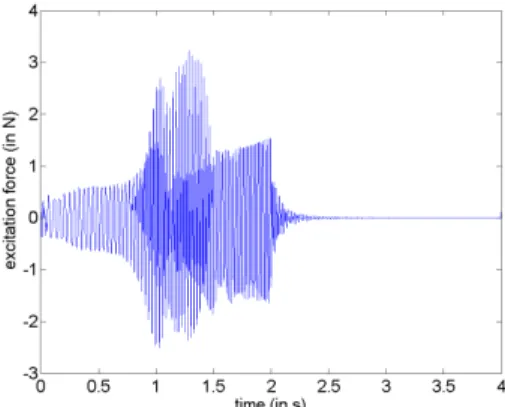
The system is excited by higher level chirp signal to put in light its nonlinear behaviour. This signal corresponds to 0.1 V applied in the signal generator. Figure 9 presents the evolution of the value of the exciting force.
Figure 9: Value of the exciting force recorded during the test and applied in the numerical model (high level chirp input).
Another metric based on the second and the third Volterra kernels is defined to update the nonlinear model (i.e. using the output corresponding to the second and the third Volterra kernels):
e F, k , c y y F, k , c
with y∗ y∗ y∗. The minimum of this nonlinear error is different from the minimum of the linear error, . The difference between both error functions can be explained by the fact that the value of these parameters – F, ks and c – have an influence on the linearised response as well as the nonlinear one. A new objective function is built to take into consideration the nonlinear behaviour of the struc-ture as well as linear part:
e e e (22)
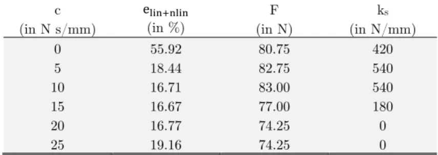
The minimum value of e as well as the corresponding value of F and ks are presented in table 2 versus c. The minimum value is obtained for: c = 15 N s mm-1, F = 77 N and ks = 180 N/mm.
c (in N s/mm)
e
(in %)
F (in N)
ks (in N/mm)
0 55.92 80.75 420
5 18.44 82.75 540
10 16.71 83.00 540
15 16.67 77.00 180
20 16.77 74.25 0
25 19.16 74.25 0
Table 2: The minimal value of e and the corresponding value of the preloaded force, F and the spring stiffness, ks versus the value of the coefficient of the viscous damper, c, for the high level chirp input.
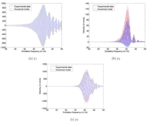
Figure 10 presents the value of the velocity recorded by the laser vibrometer and the velocity computed by the updated numerical model. The output of the updated model is very similar to the output of the experimental setup. In addition, with this model updated thanks to e , the linear error, e computed under the excitation of the low level chirp signal is close to the minimal value (see table 1). The FRF and the magnitude-squared coherence (figure 11) let us see that the numerical solution and the experimental data are close in the frequency domain. Moreover, the structure exhibit clearly a nonlinear behaviour. It can be verified that the components of both Volterra models (base on experimental data and using the updated numerical model) are also close (see figure 12). The nonlinear part of the Volterra model (y and y ) is higher than the linear one (y ). This is a clear demonstration that under the high level chirp excitation the system exhibits a nonlinear behaviour.
(a) Frequency response function (FRF) (b) Magnitude-squared coherence
Figure 11: Frequency response to the high level chirp excitation of the experimental setup and computed with the numerical model (F = 77 N, ks = 180 N mm-1 and c = 15 N s mm-1). The FRF distortions
of the plot indicate a nonlinear behaviour of the system.
(a) y1 (b) y2
(c) y3
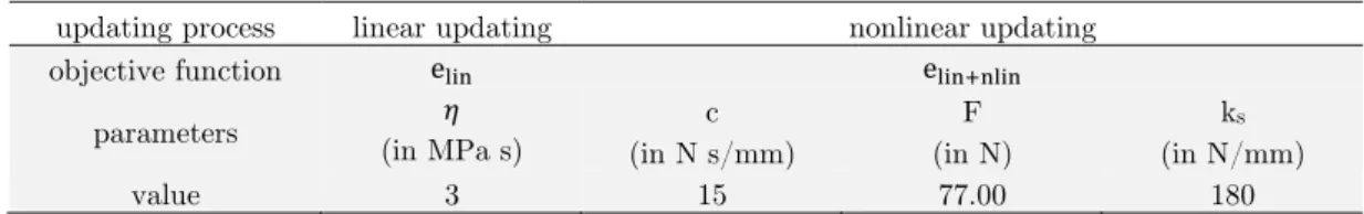
To put in a nutshell, the updating of the nonlinear finite element model is effected in two steps. First, the all parameters is evaluated thanks to the minimisation of the linear error (objective function using the first Volterra kernel). Then, only the nonlinear parameters are corrected by the minimisation of an objective function considering the three first Volterra kernels. The table 3 resume the value of the parameters identified versus the updating process and the objective function.
updating process linear updating nonlinear updating
objective function e e
parameters (in MPa s) c (in N s/mm)
F (in N)
ks (in N/mm)
value 3 15 77.00 180
Table 3: Value of the parameters identified versus the updating process and the objective function.
4.4 Validation of the Nonlinear Finite Element Model
To validate the updated nonlinear finite element model, a medium level chirp input is used. This signal is generated by 0.05 V applied in the signal generator. Figure 13(a) presents the value of the exciting force. Figure 13(b) allows us to verify that the velocity computed by the updated nonlinear model is near to the one recorded by the laser vibrometer.
(a) Value of the exciting force recorded during the test and applied in the numerical model
(b) Value of the velocity recorded by the laser vibrometer and computed by the nonlinear finite element model
Figure 13: Exciting force generated by the medium level chirp input and normal velocity in the middle of the beam recorded with the experimental setup and computed thanks to the numerical model.
on the Volterra kernels can be used for nonlinear finite element models with large number of degree of freedom.
(a) Low level (b) Medium level
(c) High level
Figure 14: Power spectral density (PSD) of the experimental setup and computed thanks to the numerical model.
5 FINAL REMARKS
In this paper, a model updating method using the Volterra series is proposed for nonlinear finite element model with large number of degree of freedom. One of the main advantages of the Volterra series is that the relationship between the input ant the output can be split into a linear response and a nonlinear one. This model updating method make use of the Volterra series to simplify the proce-dure. Consequently, this updating method is split in two parts. First, the linearised system (i.e. the
sinus-oidal signal. These examples show that the updated nonlinear finite element model essentially repro-duce the output of the experimental setup in the frequency range next to the first vibration mode which was strongly affected by the nonlinearity. In the way of reducing the computation time, the future study will be focused on the computation of the first Volterra kernel using the linearised numerical finite element model.
Acknowledgements
The authors gratefully acknowledge the financial support for this research from “Conselho Nacional de Desenvolvimento Científico e Tecnológico” (CNPq); grant number 313661/2014-6 and grant num-ber 307520/2016-1 and FAPESP; grant numnum-ber 12/09135-3. The second author is thankful to FAPESP for his scholarship grant number 13/25148-0.
References
Belytschko, T., Liu, W.K., Moran, B., Elkhodary, K., (2014). Nonlinear Finite Elements for Continua and Structures. New York: Wiley.
Bussetta, P., Shiki, S.B., da Silva, S., (2017). Nonlinear updating method: a review. Journal of the Brazilian Society of Mechanical Sciences and Engineering.
Chung, J., Hulbert, G., (1993). A time integration algorithm for structural dynamics with improved numerical dissi-pation: The generalized-α method. Journal of Applied Mechanics; 60(2):371–375. doi:10.1115/1.2900803.
Guo, Y., Guo, L.Z., Billings, S.A., Coca, D., Lang, Z.Q., (2013). Volterra series approximation of a class of nonlinear dynamical systems using the adomian decomposition method. Nonlinear Dynamics; 74(1):359–371. doi:10.1007/s11071-013-0975-8.
Kautz, W.H., (1954). Transient synthesis in the time domain. Transactions of the IRE Professional Group on Circuit Theory; 3:29–39. doi:10.1109/TCT.1954.1083588.
Kerschen, G., Lenaerts, V., Golinval, J.C., (2003). Identification of a continuous structure with a geometrical non-linearity. Part I: Conditioned reverse path method. Journal of Sound and Vibration; 262(4):889–906. doi:10.1016/S0022-460X(02)01151-3.
Kovacic, I., Brennan, M.J., editors, (2011). The Duffing equation: Nonlinear oscillators and their behaviour. John Wiley & Sons. doi:10.1002/9780470977859.
Marmarelis, V.Z., (2004). Nonlinear dynamic modeling of physiological systems. John Wiley & Sons.
Noël, J., Kerschen, G., (2017). Nonlinear system identification in structural dynamics 10 more years of progress. Me-chanical Systems and Signal Processing; 83:2–35. doi:10.1016/j.ymssp.2016.07.020.
Official website of Metafor, (2017). URL: http://metafor.ltas.ulg.ac.be/dokuwiki.
Scussel, O., da Silva, S., (2016). Output-only identification of nonlinear systems via volterra series. Journal of Vibration and Acoustics; 138(4):041012. doi:10.1115/1. 4033458.
Shiki, S.B., (2016). Application of Volterra series in nonlinear mechanical system identification and in structural health monitoring problems. Ph.D. thesis; Universidade Estadual Paulista - UNESP. URL: http://hdl.han-dle.net/11449/137761.
Shiki, S.B., Hansen, C., da Silva, S., (2014a). Nonlinear features identified by Volterra series for damage detection in a buckled beam. In: International Conference on Structural Nonlinear Dynamics and Diagnosis.
Shiki, S.B., Lopes, V., da Silva, S., (2014b). Identification of nonlinear structures using discrete-time Volterra series. Journal of the Brazilian Society of Mechanical Sciences and Engineering; 36(3):523–532. doi:10.1007/s40430-013-0088-9. Tang, B., Brennan, M.J., Lopes, J.V., da Silva, S., Ramlan, R., (2015). Using nonlinear jumps to estimate cubic stiffness nonlinearity: An experimental study. Proceedings of the Institution of Mechanical Engineers, Part C: Journal of Mechanical Engineering Science; (x):xxx–xxx. doi:10.1177/0954406215606746.
Worden, K., Tomlinson, G.R., (2001). Nonlinearity in Structural Dynamics - Detection, Identification and Modelling. University of Sheffield: Institute of Physics Publishing.