Calibration Agent for Ecological Simulations: A
Metaheuristic Approach
Pedro Valente1,2,António Pereira1,2, Luís Paulo Reis1,2
1 LIACC – Laboratório de Inteligência Artificial e Ciência de Computadores 2 FEUP – Faculdade de Engenharia da Universidade do Porto
Rua Dr. Roberto Frias s/n, 4200-465 Porto, Portugal pedro.valente@fe.up.pt
Abstract. This paper presents an approach to the calibration of ecological
models, using intelligent agents with learning skills and optimization techniques. Model calibration, in complex ecological simulations is typically performed by comparing observed with predicted data and it reveals as a key phase in the modeling process. It is an interactive process, because after each simulation, the agent acquires more information about variables inter-relations and can predict the importance of parameters into variables results. Agents may be seen, in this context, as self-learning tools that simulate the learning process of the modeler about the simulated system. As in common Metaheuristics, this self-learning process, initially involves analyzing the problem and verifying its inter-relationships. The next stage is the learning process to improve this knowledge using optimization algorithms like Hill-Climbing, Simulated Annealing and Genetic Algorithms. The process ends, when convergence criteria are obtained and thus, a suitable calibration is achieved. Simple experiments have been performed to validate the approach.
Keywords: Ecological Modeling, Calibration, Intelligent Agents, Simulation
Models, Uncertainty Analysis, Metaheuristics.
1 Introduction
The rapid progress achieved in computers hardware and software development in the last decades, have exponentially increased the usage of mathematical models across almost all fields of science, and simulation is now widely used to test or predict researchers’ theories. This is particularly relevant in the fields of physical, chemical, biological, ecological and environmental sciences, health and weather forecast domains.
Models are simplified views of processes and are used to solve scientific or management purposes. Modelers try to translate the actual knowledge about system processes, formulated in mathematical equations and components’ relationships, focusing in the processes the researcher is interested in and omitting some or many irrelevant details that aren’t important for the problem in consideration [6]. However, these omitted details may have a strong influence on the predicted results produced by the model [16].
Models are intensively used in theoretical and applied Ecology. Simulation models of complex ecological processes are increasingly constructed for use in both the development of ecological theory and the analysis of environmental questions. Such models can never be validated due to the limited observation of system dynamics [13]. They can, however, be assessed to investigate deficiencies in the relationships they define between ecological theory, model structure, and assessment data [18][16]. This study is related with ecological models of aquatic systems, for two main reasons: first, the diversity of components involved (like physical processes include flow and circulation patterns, water temperature, settling of planktonic organisms, among others), leaving to a complex ecological models, because of its interactions and dependencies. The second reason, the existence of a real simulator for coastal ecosystems – EcoDynamo [8], that permits to explore ecological models, for different point of view or interest (e. g. fishing, tourism, aquaculture, harbor activities, sports, etc.).
In the last century, human population migrates intensively from inland to coastal boundaries and, nowadays, 60% of the world lives within 60km from the sea. So the correct management of the coastal zones is very important for the environment balance, and sustainable development [4].
Computer Simulation is a powerful tool in evaluating complex systems, like Coastal ecosystems. These evaluations are usually in the form of responses to “what if” questions. Practical questions, however, are often of “how to” nature. “What if” questions demand answers on certain performance measures for a given set of values for the decisions variables of the system. “How to” questions, on the other hand, seek optimum values for the decision variables of the system so that a given response or a vector of responses are maximized or minimized [2][19].
Using simulation as an aid for optimization presents several specific challenges. Some of these issues are those involved in optimization of any complex and highly nonlinear function. Others are more specifically related to the special nature of simulation modeling. Simply acknowledged, a simulation optimization problem is an optimization problem where the value of the objective function (objective functions, in case of a multi-criteria problem) and/or some constrains, can only be evaluated by computer simulation, and its validity made by compare it to real data. However, these functions are only implicit functions of decision parameters of the system. In sum, these functions are often stochastic1 in nature as well.
Considered these characteristics in mind, for example, the objective function(s) and these constraints are stochastic functions of deterministic decision variables. These leave a major problem in estimation of even approximate local derivatives. Furthermore, this work against even using complete enumeration because based on just one observation at each point the best decision point cannot be determined. This is a generic non-linear programming problem.
However, advantages in using simulation optimization, for example, in stochastic systems, like ecological ones, the variance of the response is controllable by various output analysis techniques. Other main strength in using optimization techniques,
1 Stochastic - A process with an indeterminate or random element as opposed to a deterministic process that has no random element.
reflect the constant change of objective function or constraints from one interaction to another to reflect alternative designs for the systems [19][13].
Those optimization techniques or Metaheuristics can be more intuitive, if previous, by observing simulated model runs, we learn how variables interact, and the sensitivity of tune parameters values. In this case, optimization techniques don’t test in all space available, but in sub-space of pre-known validation [20].
The paper is organized as follows: the next section describes in more detail the problem in analysis; section 3, introduces and presents the key features of some known Metaheuristics: hill-climbing, Simulated Annealing and Genetic Algorithms; section 4 presents the architecture of the multi-agent simulation system, and its components; section 5 focus into Calibration Agent and it’s methodology applied to an ecological model; the paper concludes with some conclusion and analysis of the project current state and pointers to future work.
2 Problem Statement
One of the problems related in simulated modeling is the lack of fitness in results produced and the real data sets, because a model represents a wider view of reality, in this particularly case, an ecosystem. All models are translated by mathematical formulas, in which main variables are represented. The validation formulas process, are made by specialist, whose sensibility and comprehension on ecological systems, result into better fit to real ones.
The formula validation process made by specialist, basically consist into change parameters values, and compare the result variables with observed data. It is a methodic process of recombination values into optimal results.
When models became complex, with various formulas, parameters and variables, that can be combine or reused, the process of tuning became complex and time consuming. In these cases, use of Parameter Optimization and Simulation Optimization became one of best problem solution.
An optimization problem normally consists on trying to find values, of free parameters of a system, in which objective function is maximized (or in some cases minimized.
Several problems resolutions can be made by searching the best configuration set of parameters, which fulfill the goal (or some goals). The goal is either to minimized or maximized some quantity. This quantity is express by a function f, of one or more variables known as the objective function.
Variables that can change in the quest for optimality are known as the decision variables. If goal is to minimize then f is known either as the cost function or the penalty function. In opposition, when the goal is maximization, f is referred as the benefit function or utility function.
These problems, classified into optimizations problems, are important in both theoretical and practical domain. In some case, the values of decision variables can be specified through a number of conditions - the constraints. For example, the range number in a variable can be considered as constraint, in which function f must take in consideration.
The search space of a problem is defined as the set of all candidate solutions. Each candidate solution is express by an instantiation of decision variables, and therefore by a quantity or objective function result. It is considered feasible solution or just a solution, if a candidate satisfies all constraints of the problem. The search space is formed by all feasible solutions.
Simulation Optimization procedures are used when our objective function can only be evaluated by using computer simulations. This happens because there is not an analytical expression for our objective function, ruling out the possibility of using differentiation methods or even exact calculation of local gradients. Normally these functions are also stochastic in nature, causing even more difficulties to the task of finding the optimum parameters, as even calculating local gradient estimates becomes complicated.
Running a simulation is always computationally more expensive than evaluating analytical functions thus the performance of optimization algorithms is crucial.
Theoretical problems with calibrating complex models is highlighted by Villa et al. [19] who developed and applied a computer aided search algorithm for exploring model parameter spaces, and compared these explorations against more usual methods of calibration such as eyeballing, hill climbing and Monte Carlo experiments. Villa et al. [19] found that as the number of unknown parameters increases, the number of areas that can be discriminated within the parameter space to fit the same observed data is also increasing. When less is known of a modeled system, systematic calibration of complex models will reveal more potential solutions. Consequently, non systematic calibrations, such as ‘eyeballing’, have been inconclusive as methods for exploring the total potential parameter space.
3 Optimization and Metaheuristics
There are several situations where one has to deal with problems of growing complexity. These problems arise in diverse areas of knowledge. Often, the problem to be solved can be expressed as an optimization problem where, for each particular instance, the goal is to find a solution which minimizes (or maximizes) a given objective function [5].
Optimization problems are commonly divided into two main categories [5]: those where solutions are encoded as real numbers; and those where solutions are encoded as discrete values. Amongst the later class, a prominent group is that of combinatorial optimization problems, where the objective is to find an optimal combination of solution components from a finite (or possibly countable infinite) set.
For some optimization problems either there is no knowledge how to definitively find a global optimum or the known algorithm has no practical usefulness due to its computational effort. They are known as being of difficult optimization [1][14][7]. For such cases, approximate algorithms play an important role [16]. Although they not (generally) guarantee that a global optimum would be found, they are (usually) able to find sub-optimal solutions within small time budgets.
For discrete problems several heuristics have been developed along the years in order to produce high quality solutions. The majority of them were conceived to solve
a particular problem. Thus, some of the considerable effort putted in the development and refinement of such heuristics is more likely to be wasted if a (slightly) different problem has to be solved.
Metaheuristics are algorithmic frameworks that, at some extent, can be applied to a multiplicity of problems without major modifications [5]. They are in fact general high-level heuristics that guide an underlying search strategy in order to intelligently explore the solution space and return high quality solutions.
3.1 Hill-climbing
One of the principles behind Metaheuristic, is the definition of a neighbourhood leads to the definition of locally optimal solutions, or simply local optima. A local optimum is a feasible solution whose objective function is optimal in respect to a given neighbourhood, i.e. none of its neighbours have a better evaluation of the objective function [14].
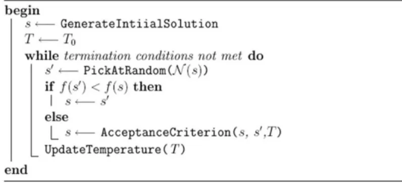
The most obvious local search strategy is iterative improvement (known as hill-climbing in the case of maximization). Given an initial solution and a neighbourhood relation, the iterative improvement strategy moves to a neighbour if and only if it corresponds to an improvement of the objective function. The search process continues from the found better solution and iterates until no improvement is possible. The algorithmic skeleton of iterative improvement is depicted in figure 1.
Fig. 1. Hill-Climbing Algorithm.
3.2 Simulated Annealing
Simulated Annealing (SA), also known as Monte Carlo annealing and statistical cooling, is a stochastic local search metaheuristic. It was one of the first algorithms incorporating an explicit mechanism to escape from local optima [7].
Its motivation arises from the physical annealing of solids. Annealing is a thermal treatment applied to some materials (e.g. steel, brass, glass) in order to alter their microstructure, affecting their mechanical properties. The annealing process starts by initially raising the temperature of a substance to high values (melt point). At this state the particles of the substance are arranged randomly. Then, carefully proceeds with a slow cooling process spending long times at temperatures in the vicinity of the freezing point. This process allows the substance to solidify with a crystalline structure, a perfect structure that corresponds to a state of minimum energy – the ground state.
Fig. 2. Simulated Annealing Algorithm.
SA uses the physical annealing analogy to solve optimization problems [7]. In this analogy, the candidate solutions of the optimization problem have correspondence with the physical states of the matter, where the ground state corresponds to the global optimum (minimum). The objective function corresponds to the energy of the solid at a given state (see figure 2). The temperature initialized to a high value and then decreased during the search process, has correspondence, into some extent, to the iteration count.
The fundamental idea of SA is to make a walk based on a local search strategy but allowing accepting solutions worse than the current one. This provides the algorithm with a good mechanism to escape from local optima [7].
3.3 Genetic Algorithms
Genetic algorithms are adaptive methods, which may be used to solve search and optimization problems [23][1]. They are based on the genetic process of biological organisms. Over many generations, natural populations evolve according to the principles of natural selection, i.e. survival of the fittest, first clearly stated by Charles Darwin in The Origin of Species. By mimicking this process, genetic algorithms are able to evolve solutions to real world problems, if they have been suitably encoded [23].
Before a genetic algorithm can be run, a suitable encoding (or representation) for the problem must be devised. A fitness function is also required, which assigns a figure of merit to each encoded solution. During the run, parents must be selected for reproduction, and recombined to generate offspring (see Figure 3).
Fig. 3. Genetic Algorithm.
Termination conditions of the algorithm can vary. If there is a known optimal value to the fitness function an obvious choice is to stop when that value is reached (or at least within a given precision). However this criterion has usually to be extended due to several factors: the optimal value is unknown, there are no guarantees to reach the optimal value within a given time limit (or there are no guarantees at all). So, termination condition has to include some condition that indubitably stops the algorithm.
4 Simulation System Architecture
The simulation system framework, named EcoSimNet, was built to enable physical and biogeochemical simulation of aquatic ecosystems [8][9][10][11][12][3]. The core application, the simulator EcoDynamo [8], is an object-oriented program application, built in C++ and is responsible to communicate between model classes and the output devices where the simulation results are saved. The simulated processes include [9]:
• Hydrodynamics of aquatic ecosystems – current speeds, and directions; • Thermodynamics – energy balances between water and atmosphere and
water temperature;
• Biogeochemical – nutrient and biological species dynamics; • Anthropogenic pressures, such as biomass harvesting.
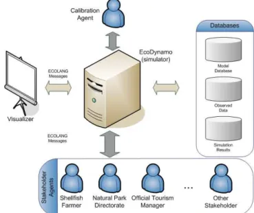
Fig. 4. Agent-based Simulation System Architecture.
Figure 4 defines the EcoSimNet architecture. The simulator has a graphical interface, where users can interact with ecological model properties: definitions as
morphology, geometric representation of the model, dimensions, number of cell, classes, variables, parameter initial values and ranges. The user have the power to choose the model, which classes it simulates, the period of time simulated, and the period of time to output results for file or chart. The output files are compatible with major commercial software, for posterior treatments and the charts are generated by MatLab®.
Each model is influenced by its class, objects that represent real entities behavior, like wind, tidal current, dissolved substances, etc. Different classes simulate different variables and processes, with proper parameters and process equations. All data are kept in database files, for posterior comparison with observed data.
This framework has the capacity to extend functionalities by adding external/remote applications (typically the Agents)[21]. All applications communicate with simulator by a TCP/IP communication protocol using ECOLANG language [12] (the EcoSimNet protocol), defining all semantic messages necessary for management and simulation domain. Allow the interaction between ecological simulation experiments and several agents, representing either users of the system under simulation or applications designed to perform specific modeling tasks.
All Agents can do the same tasks as the users do with the simulator (start/stop the model simulation runs - start, stop, pause, restart and step – select classes, collect variables to output).
The visualization application interacts with simulator, representing graphically (2D or 3D) the morphology and stakeholders agents’ interaction. The user can see information valid about classes simulated in some unit space (so called boxes).
5 Calibration Agent
Several procedures for automatic calibration and validation are available in the literature, like the Controlled Random Search (CRS) method [16] or the multi criteria model assessment methodology, Pareto Optimal Model Assessment Cycle (POMAC) [14]. However, these procedures do not capture the complexity of human reasoning in calibration process. They try to explore all search spaces, leaving to computer time consuming without best results.
The Calibration Agent (CA) is an Intelligent Agent [15][22] that communicates through the EcoSimNet protocol with the simulation application, assuming control over primary tasks around model understanding (ie. read/change model parameters, run simulation, collect results, etc…). Its purpose is to tune model equation parameters in order to fit the model to observed data, towards model calibration and validation.
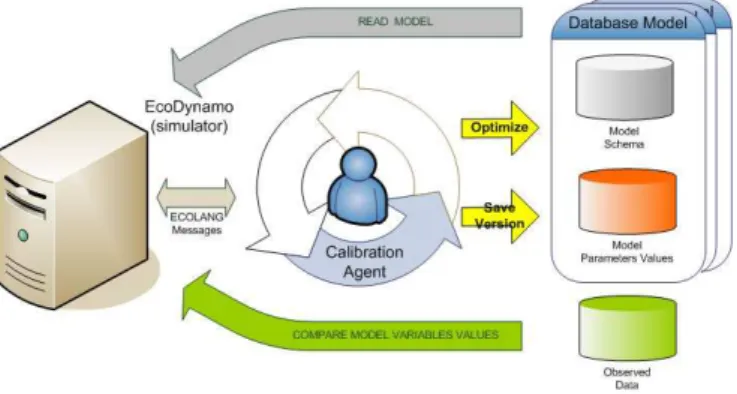
Fig. 5. Calibration Agent System Architecture.
All communications are made with simulator, using ECOLANG messages to compute input/outputs for the model loaded by application.
The CA acquires knowledge about the behavior of the system processes in five steps (see figure 5): 1) Simulator loads from Database Model, the schema and initial parameters values for model equation, 2) CA acquires the list of parameters and their values, 3) change the values of the parameters, using some knowledge based techniques, 4) run simulation model and 5) compare the lack of fitness between variables values simulated and observed ones.
The process finishes when the criteria of convergence is obtained or the user, in the graphical interface, stops the optimization. The user can save the parameter’s vector of values, into the model database (Model Parameters Values Database), to load it in a new optimization, like the first step of the process.
This process is interactive, and its success depends, almost completely on the process of selecting the right parameter and their correct values. For this reason, the use of intelligent agents makes all the difference, because of its capacity of learning and change its strategies at any time of the computing cycle.
The knowledge about the behavior of all system processes, until these days restrained for the experts, or “modeler” in the traditional calibration process, shall be used to guide the selection of new values for the parameters contained in different mathematical relationships. It is important to understand the flow inside mathematical expressions for better calibration. From simulator, CA only knows the model classes (entities simulated), the variables (result from expressions) inside them and the values of the parameters. In the present system, the CA, learn knowledge model in three phases [9]:
• Capturing relationships among classes and inter-variable;
• Analyzing the intra and interclass sensitivity of different variables to different parameters and among variables;
• Iterative model execution (run simulation), measuring model lack of fit, adequacy and reliability, until a convergence criteria is obtained.
These phases make the methodology more robust with the minimal understanding of model flow, and can be transposed to others models. The complete calibration procedure is show in Figure 6.
Fig. 6. Calibration Agent Procedure diagram [9]
The first step in CA is choosing the model to tune. This task became simplified, because the model loaded, for CA, is choosed by user interface in the simulator, and all extern modules read the same model.
Step1 and 2 from the diagram represent the understanding phase model. In these steps relationships matrix for classes and variables inside the same class and inter-class are constructed.
How can the CA know for each class variable, the interaction with others variables? This process is simplified because there are 2 internal simulator messages that reveal relationships: Inquiry and Update methods. Each class that interacts in ecosystem could know the values of variables in others entities – using the Inquiry method. If some class influences another uses the Update method for change some variable value in the other class, like in predator/prey model, where one class influences the other and vice-versa [6].
After this acquisition information or knowledge, by run model simulation for some period of time, the agent has in its power the minimal understanding how the entities model flow in the simulation.
After this phase the tuning process begins, applying the Metaheuristics algorithms related above. The optimization algorithm runs in search the adequate parameters values, not randomly but following the matrix of relationships constructed prior. The choice of optimization algorithms is influenced by the number of variables/parameters unknown that the model deals. Each optimization algorithm is tuned and combined with another Metaheuristics technique, to give the best values, in the valid time period.
6 Conclusions and Future Work
Model calibration is performed by comparing observed with predicted data and is a crucial phase in the modelling process. Because it is an iterative and interactive task in which, after each simulation, the expertise (or modeller) analyses the result and changes one or more equation parameter trying to tune the model, this “tunning” procedure requires a good understanding of the effect of different parameters over different variables. This is particularly painful in the simulation of ecological models, where the physical, chemical and biological processes are combined and the values of various parameters, which integrates the functions of the processes, are only estimated and may vary within a range of values commonly accepted by the researchers.
Using a calibration agent for model tuning enables full automate a very complex and tedious problem to solve manually, and without change the simulation code application. Because it is an agent, it can “live” abroad of core simulation and it is easier to upgrade the parameter tune techniques.
With this approach, we considered that some knowledge is gained into step 1 and 2 of the agent procedure diagram, but it is not trivial to compare the influence of parameters in variables between classes.
Simple controlled experiences have been made to test the validity of this approach for model calibration. However in terms of Metaheuristics, and model complexity, we can take result of other optimization techniques, like reinforcement learning.
The result of this work will be applied in the calibration of the Ria Formosa (Algarve) ecological model, in the context of ABSES project.
Acknowledgments
This work is partially supported by the ABSES project – “Agent-Based Simulation of ecological Systems”, (FCT/POSC/EIA/57671/2004).
References
1. Beasley, D., Bull, D.R. and Martin, R.R. (1993). An Overview of Genetic Algorithms: Part 1, Fundamentals, University Computing, Vol. 15, No.2, pp. 58-69, Department of Computing Mathematics, University of Cardiff, UK.
2. Beven, K., Binley, A., 1992. The future of distributed models: model calibration and uncertainty prediction. Hydrological Processes 6, 279–298.
3. Cruz , F., Pereira, A., Valente, P., Duarte , P. and Reis, L. P.: Intelligent Farmer Agent for Multi-Agent Ecological Simulations Optimization. In: J. Neves, M. Santos and J. Machado (eds): EPIA 2007, LNAI 4874, pp.593-604, 2007. Springer-Verlag, Berlin Heidelberg. ISBN: 978-3-540-77000-8 (doi:10.1007/978-3-540-77002-2_50).
4. Duarte, P., Meneses, R., Hawkins, A.J.S., Zhu, M., Fang, J., Grant, J.: Mathematical modelling to assess the carrying capacity for multi-species culture within coastal waters. Ecological Modelling 168, 109–143 (2003).
5. Glover, Fred; Kochenberger, Gary - Handbook of Metaheuristics (International Series in Operations Research & Management Science). Springer, 2003.
6. Jørgensen, S. E. and Bendoricchio, G.: Fundamentals of Ecological Modelling. Elsevier Science Ltd, 3rd edition. 2001.
7. Kirkpatrick, S.; Gelatt, C.; Vecchi, M. Optimization by Simulated Annealing, Science, 220 (4598), pp. 671-680, 1983.
8. Pereira, A. and Duarte, P.: EcoDynamo – Ecological Dynamics Model Apllication (Technical Report), University Fernando Pessoa, 2005.
9. Pereira, A., Duarte, P., Reis, L.P.: Agent-based Ecological Model Calibration – On the Edge of a New Approach. In: Ramos, C. and Vale, Z. (eds.), Proceedings of the International Conference on Knowledge Engineering and Decision Support, pp. 107-113, ISEP, Porto, Portugal, July. ISBN: 972-8688-24-5.
10. Pereira, A., Duarte, P., Reis, L.P.: Agent-Based Simulation of Ecological Models. In: Coelho, H., Espinasse, B. (eds.) Proceedings of the 5th Workshop on Agent-Based Simulation, Lisbon, pp. 135–140 (2004)
11. Pereira, A., Duarte, P., Reis, L.P.: An Integrated Ecological Modelling and Decision Support Methodology. In: Zelinka, I., Oplatková, Z., Orsoni, A. (eds.) 21st European Conference on Modelling and Simulation, ECMS, Prague, pp. 497–502 (2007)
12. Pereira, A., Duarte, P., Reis, L.P.: ECOLANG – A Communication Language for Simulations of Complex Ecological Systems. In: Merkuryev, Y., Zobel, R., Kerckhoffs, E. (eds.) Proceedings of the 19th European Conference on Modelling and Simulation, Riga, pp. 493–500 (2005)
13. Reynolds, J. H., Ford, E. D. - Multi-Criteria Assessment of Ecological Process Models. Washington: Currently Department of Statistics, University of Washington,, 1998. NRCSE-TRS No. 010.
14. Roberts, M., Howe, A. and Whitley, L.D.: Modeling Local Search: A First Step Toward Understanding Hill-climbing Search in Oversubscribed Scheduling. IN: American Association for Artificial Intelligence (www.aaai.org), 2005.
15. Russel, S., Norvig, P.: Artificial Intelligence: A modern approach, 2nd edn. Prentice-Hall, Englewood Cliffs (2003).
16. Scholten, H. and van der Tol,: Quantitative Validation of Deterministic Models: When is a Model Acceptable?. Proceedings of Summer Computer Simulation Conference, 404-409, SCS int., San Diego, CA, USA (July 12-22, 1998, Reno, Nevada, USA)
17. The DITTY project description [online]. Available at http://www.dittyproject.org [visited January, 8, 2008]
18. Thomas Back and Hans-Paul Schwefel. Evolutionary computation:An overview. In T. Fukuda, T. Furuhashi and D. B. Fogel, editeur, Proceedings of 1996 IEEE International Conference on Evolutionary Computation (ICEC '96), Nagoya, pages 20{29, Piscataway NJ, 1996. IEEE Press.
19. Villa, F., Boumans, R.M.J., Costanza, R., 1998. Calibration and testing of complex process-based simulation models. Proceedings of the Applied Modeling and Simulation (AMS) Conference, Honolulu, 12–14 August 1998.
20. Wang, Q.L., 1997. Using genetic algorithms to optimize model parameters. Environmental Modeling and Software 12 (1), 27–34.
21. Weiss, G.: Multiagent Systems. MIT Press, Cambridge (2000).
22. Wooldridge, M.: An Introduction to Multi-Agent Systems. John Wiley & Sons, Ltd., Chichester (2002).
![Fig. 6. Calibration Agent Procedure diagram [9]](https://thumb-eu.123doks.com/thumbv2/123dok_br/14922488.1000002/10.892.332.561.221.493/fig-calibration-agent-procedure-diagram.webp)
