New strategies to detect and understand genotype-by-environment interactions and QTL-by-environment interactions

(1)

Mestre

New strategies to detect and understand

genotype-by-environment interactions

and QTL-by-environment interactions

Dissertação para obtenção do Grau de Doutor em Estatística e Gestão do Risco, especialidade em Estatística

Orientador: Stanislaw Mejza, Full Professor, Poznan

University of Life Sciences, Poland

Co-orientador: João Tiago Mexia, Jubilee Full Professor,

FCT-UNL, Portugal

Júri:

Presidente: Prof. Doutor Fernando José Pires Santana Arguente(s): Prof. Doutor Hans-Peter Piepho

Prof. Doutora Ana Maria Nobre Vilhena Pires Parente

Vogais: Prof. Doutora Maria Antónia Amaral Turkman Prof. Doutor Carlos Manuel Agra Coelho

Prof. Doutor Stanislaw Mejza

Prof. Doutor João Tiago Praça Nunes Mexia

(2)

(3)

Mestre

New strategies to detect and understand

genotype-by-environment interactions

and QTL-by-environment interactions

Dissertação para obtenção do Grau de Doutor em Estatística e Gestão do Risco, especialidade em Estatística

Orientador: Stanislaw Mejza, Full Professor, Poznan

University of Life Sciences, Poland

Co-orientador: João Tiago Mexia, Jubilee Full Professor,

FCT-UNL, Portugal

Júri:

Presidente: Prof. Doutor Fernando José Pires Santana Arguente(s): Prof. Doutor Hans-Peter Piepho

Prof. Doutora Ana Maria Nobre Vilhena Pires Parente

Vogais: Prof. Doutora Maria Antónia Amaral Turkman Prof. Doutor Carlos Manuel Agra Coelho

Prof. Doutor Stanislaw Mejza

Prof. Doutor João Tiago Praça Nunes Mexia

(4)

(5)

Copyright

(6)

(7)

Acknowledgements

The last four and half years were (mostly) great and challenging! I had the great chance to work with many people and to visit many places during this journey. It is a pleasure to thank now to those who made the end of this thesis possible, either because of their scientific or emotional support.

First of all I would like to thank to my Mentors who share their knowledge with me and contributed greatly for my development as a researcher and as a person:

 to my supervisors Stanislaw Mejza and João Tiago Mexia. Professor Mexia and Professor Mejza were with me since the beginning, and have done everything they could to help me in any way I

needed. I’m deeply grateful to them for all the help and unconditional support. I’m very glad I can

have them by my side, as friends and collaborators. They are always there!

 to Hugh G. Gauch. Hugh definitively was one of the most important people for me in these years! His contribution to my scientific and personal development was immeasurable. He was great and even without knowing me or asking for any reference he accepted me as his guest in Cornell and shared his office with me. Hugh spent a lot of time with me discussing real science and the reasons why we do that. I’m deeply thankful for having the chance of meeting and really get to know him. Hugh is the best person I have ever met and represents what all people (including researchers) should

be like. I have no doubts I’m a better person now because of him.

 to Fred van Eeuwijk. I had the chance to work with Fred in Wageningen for about two years, which really contributed for my development in many ways. We had great meetings where I learned a lot

from our discussions and from his great knowledge in this topic. I’m really thankful to Fred for giving

me the supervision, to wrap up this thesis and for the great support in the final stage of this thesis. He contributed greatly for a better outcome.

I also would like to thank all my Co-Authors which in one way or in other helped me to finish the chapters of this thesis and improve my knowledge on several topics.

Besides my Mentors and Co-Authors, I had the chance to meet great people and make very good friends I hope to keep. In CMA we had a great environment created by a few good friends: Miguel Fonseca, Miguel de Carvalho, Elsa, Agostinho, Sandra and Vanda. In Poznan I have also found great people I can now call friends, namely Kasia, Ania and Aga. They were great and I felt at home in Poznan. In Wageningen I really enjoyed the company and conversations with Paul, Sabine, Nurudeen, Maria João, Marcos, Alba, Noor and

the great “football people” who work in the research group of Organic Farming Systems. I’ll definitively

miss our matches! I thank all of them and many others not mentioned for the enjoyable time I spend with them!

I must not forget the financial support which allowed me to reach this end. I would like to thank Fundação para a Ciência e Tecnologia (Portuguese Foundation for Science and Technology), of Ministério da Ciência, Tecnologia, e Ensino Superior, Portugal, for my doctoral grant SFRH/BD/35994/2007, which lasted for four years. I would also like to thank the project N N310 447838 supported by Ministry of Science and Higher Education, Poland, for further financial support.

(8)

(9)

Resumo

Interação entre genótipo e ambiente (GEI) é frequente em ensaios multi-localização, e traduz-se por

diferentes respostas dos genótipos em diferentes ambientes. Com o desenvolvimento das marcas

moleculares e técnicas de mapeamento, os investigadores podem analisar todo o genoma para detectar as

localizações específicas dos genes que influenciam a característica quantitativa de interesse. Estas localizações

são denominadas de quantitative trait locus (QTL) e, quando estes QTLs apresentam diferentes respostas em

diferentes ambientes, estamos perante interações entre QTL e ambiente (QEI), que é a base da GEI. Uma

boa compreensão destas interações permite aos investigadores selecionar melhores genótipos para diferentes

condições ambientais e, consequentemente, melhorar colheitas em paises desenvolvidos e, especialmente, em

países em desenvolvimento. Nesta tese de doutoramento pretendo apresentar novas estratégias para

melhorar a deteção e perceção de QTLs, especialmente QTLs associados a QEI no contexto de ensaios

multi-localização, utilizando e fornecendo open source software.

Na primeira parte desta tese é apresentada uma comparação entre dois dos métodos mais usados na

análise da GEI: a análise conjunta de regressões (JRA) e o modelo de efeitos principais aditivos e interação

multiplicativa (AMMI). Esta comparação é realizada em termos de “robustez” com o aumento da proporção

de valores omissos, e em termos da obtenção dos genótipos dominates/vencedores. Nos capítulos seguintes

são apresentados métodos com duas e três etapas onde os modelos AMMI são usados para aumentar a

precisão dos dados fenotípicos, e os respectivos scores usados para ordenar os ambientes na procura de

padrões ecológicos ou biológicos. A primeira destas abordagens (duas etapas) é apropriada quando a

variância do erro é constante ao longo dos ambientes, enquanto a segunda (três etapas) é uma generalização

permitindo ter em conta diferenças na variância do erro ao usar o modelo AMMI ponderado (WAMMI,

proposto nesta tese). A parte final da tese ilustra uma estratégia para simular e modelar GEI e QEI em

características complexas como a produção/rendimento, com base numa série de parâmetros fisiológicos

dependendo apenas dos dados genotípicos. Isto é realizado usando um modelo eco-fisiológico de

crescimento de colheitas com sete parâmetros dependentes de QTLs.

(10)

(11)

Abstract

Genotype-by-environment interaction (GEI) is frequent in multi-environment trials, and represents

differential responses of genotypes across environments. With the development of molecular markers and

mapping techniques, researchers can go one step further and analyse the whole genome to detect specific

locations of genes which influence a quantitative trait such as yield. These locations are called quantitative

trait locus (QTL), and when these QTLs have different expression across environments we talk about

QTL-by-environment interactions (QEI), which is the base of GEI. Good understandings of these interactions

enable researchers to select better genotypes across different environmental conditions and, consequently, to

improve crops in developed and developing countries. In this thesis I intend to present new strategies to

improve detection and better understanding of QTLs, especially those exhibiting QEI in the context of

multi-environment trials, by using and providing open source software.

The first part of this thesis presents a comparison between two of the most used methods to analyse and

to structure GEI: the joint regression analysis (JRA) and the additive main effects and multiplicative

interaction (AMMI) model. This comparison is made in terms of “robustness” with different incidence rates of missing values, and in terms of dominant/winner genotypes. In the following chapters two- and

three-stages approaches are presented in which the AMMI model is used to gain accuracy in the phenotypic data,

and their scores used to order the environments to find ecological or biological patterns. The first approach

(two stages) is appropriated when the error variance is constant across environments, whereas the second

(three stages) is more general and accounts for differences in the error variances by using the proposed

weighted AMMI model (WAMMI). The final part of the thesis illustrates a strategy to simulate and to model

GEI and QEI in complex traits, with the example of yield, based on a number of physiological parameters

purely genotype dependent. This is done by using an eco-physiological genotype-to-phenotype model with

seven parameters defined with a simple QTL basis.

(12)

(13)

List of Figures

Figure 1.1. Number of publications about GEI, QEI, QTL and G-P models, per year. ... 2

Figure 1.2. Proportion of publications about QEI within the number of publications about QTLs, per year. ... 2

Figure 1.3. Number of publications on research about GEI, per statistical method, per year. ... 3

Figure 2.1. Upper contour with the four dominant genotypes in the durum wheat population. ... 15

Figure 2.2. Ockham's hill for accuracy of the yield estimates for the durum wheat experiment. ... 21

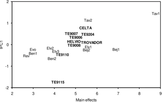
Figure 2.3. AMMI1 biplot for the durum wheat experiment. ... 22

Figure 3.1. AMMI1 biplot for 2004. ... 36

Figure 4.1. QTL scans for the 11 environments of the wheat PHS experiment ordered by location and year ... 48

Figure 4.2. QTL scans for the main effects and IPC1 to IPC3 for the wheat PHS experiment ... 49

Figure 4.3. Ockham’s valley for the wheat PHS experiment ... 50

Figure 4.4. QTL scans for Ketola 2004 based on the AMMI1 estimates and the raw data or naïve estimates. ... 51

Figure 4.5. The AMMI1 biplot for the wheat PHS experiment. ... 52

Figure 4.6. QTL scans for the 11 environments of the wheat PHS experiment, with the environments ordered by the environment IPC1 scores. ... 53

Figure 4.7. QTL expression as a function of environment IPC1 scores for the wheat PHS experiment. ... 55

Figure 4.8. Ockham’s hill for QTL detections for the wheat PHS experiment. ... 57

Figure 4.9. The AMMI2 biplot for the barley yield experiment. ... 61

Figure 4.10. QTL scans for the 16 environments of the barley yield experiment. ... 62

Figure 4.11. QTL expression as a function of environment PC1 scores for the barley yield experiment. ... 64

Figure 5.1. Schematic diagram of the crop growth model with seven physiological parameters. ... 72

Figure 5.2.Genetic map for pepper. ... 75

Figure 5.3. GGE biplot for one random realization of the two-way table... 80

Figure 5.4. AMMI2 biplot for one random realization of the two-way table. ... 81

Figure 6.1. QTL scans for 6 environments of the yield data for pepper. ... 97

Figure 6.2. AMMI2 and WAMMI2 biplots for one randomly chosen realization. ... 98

Figure 6.3. Summary of the number of detected QTLs for the actual data, AMMI2 predicted values, WAMMI2 predicted values and linear mixed model... 99

Figure 6.4. Number of QTLs detected per environment. ... 100

Figure 6.5. QTL scans for the 13 environments for the means of the SxM yield data, AMMI3 predicted values, and WAMMI3 predicted values. ... 101

Figure 6.6. Biplots for the first two axes of AMMI3 and WAMMI3 models, for the SxM yield data. ... 102

Figure 6.7. Genetic map with the information of the place where a QTL was detected for the SxM yield data. ... 104

Figure 7.1. Parents (Yolo Wonder and CM334) and F1 of the recombined inbred lines of pepper population and glasshouse experiments. ... 114

Figure 7.2. Observed and simulated yield for the pepper population in SP1 and SP2. ... 115

(18)

(19)

List of Tables

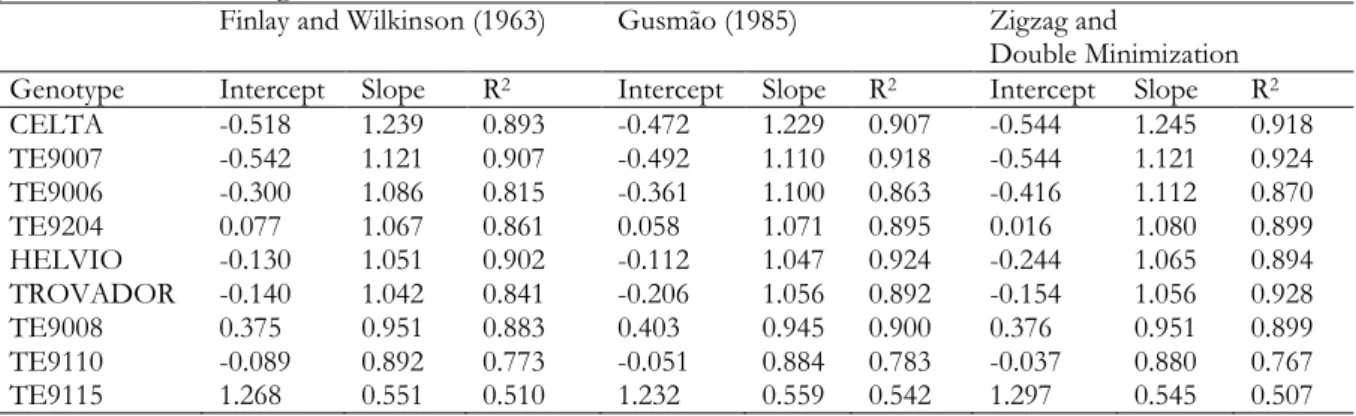
Table 2.1. Adjusted regression coefficients and coefficients of determination. ... 18

Table 2.2. Sums of the sums of squares of residuals. ... 19

Table 2.3. Dominant and number of significantly dominated genotypes for JRA, environments where the genotypes were dominant (JRA) and where the genotypes were winners (AMMI)... 20

Table 2.4. AMMI4 analysis of variance. ... 21

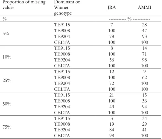
Table 2.5. Proportion of runs in which dominant genotypes (JRA) and winners of mega-environments (AMMI) are common to the results of the original data ... 24

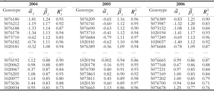
Table 3.1. Adjusted regressions coefficients and coefficients of determination, ordered by slope in each year. ... 32

Table 3.2. The dominant genotypes, range of dominance, environments where the genotypes are dominant and the number of significantly dominated genotypes for 2004. ... 33

Table 3.5. Results of the ANOVA for the AMMI5 model in 2004... 35

Table 3.6. Results of the ANOVA for the AMMI5 model in 2005... 36

Table 3.7. Results of the ANOVA for the AMMI5 model for 2006... 38

Table 3.8. Model comparison for predict ability for yield in spring barley for 2004, 2005 and 2006... 39

Table 4.1. Main QTLs for preharvest sprouting. ... 47

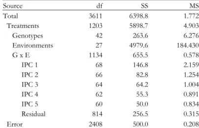
Table 4.2. AMMI3 analysis of variance for the preharvest spouting scores of the cross Cayuga x Caledonia. ... 49

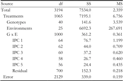
Table 4.3. AMMI7 analysis of variance for the yield of the cross Steptoe x Morex. ... 59

Table 5.1. The seven genotype specific, environment independent physiological parameters in the yield model, parameterized for greenhouse sweet pepper. ... 74

Table 5.2. Parameterization of the constants in the model for sweet pepper. ... 74

Table 5.3. Genetic architecture in the eco-phisiological genotype-to-phenotype model. ... 76

Table 5.4. Sensitivity analysis for the physiological parameters and environmental characterizations. ... 79

Table 5.5. ANOVA for the AMMI model with 2 interaction principal components. ... 80

Table 5.6. QTL effects and standard errors for the 10 detections for several subsets of environments. ... 83

Table 6.1. The 12 environments used in the simulated yield data for pepper. ... 92

Table 6.2. Genetic architecture of the simulated yield data for pepper (signal).. ... 92

Table 6.3. The 13 environments used in the SxM analysis. ... 93

Table 6.4. ANOVA of the AMMI5 model for the simulated yield data for pepper. ... 97

(20)

(21)

List of Abbreviations

AMMI – additive main effects and multiplicative interaction ANOVA – analysis of variance

AQ – AMMI analysis followed by QTL scans CxC –‘Cayuga’ × ‘Caledonia’

CIM – composite interval mapping df – degrees of freedom

DH – doubled haploid

EM – expectation-maximization FDMC – fruit dry matter content FTF – fraction to fruits

GEI – genotype-by-environment interactions

GGE – genotype main effect plus genotype by environment interaction GLI – genotype-by-location interactions

G-P – genotype-to-phenotype

IPC – interaction principal component JRA – joint regression analysis

LOD – logarithm of odds LUE – light use efficiency MET – multi-environment trial MS – mean square

PCA – principal components analysis PHS – preharvest sprouting

QEI – QTL-by-environnement interaction QTL – quantitative trait locus

RMSPD – root mean square predictive difference S×M –‘Steptoe’ × ‘Morex’

S/N – signal to noise SREG – sites regression SS – sum of squares

SVD – singular value decomposition

(22)

(23)

Chapter 1 General Introduction

1.

Introduction

1.1.

One of the main challenges in statistical genetics is to find superior genotypes over a wide range of

agro-ecological conditions and also over a number of years. This is also a challenge for farmers, breeders and

geneticists although farmers and breeders have often conflicting interests: breeders want genotype that can

be sold everywhere and farmers a genotype adapted to their climate and soil management. To achieve this

purpose, multi-environment trials (METs) are conducted in which a series of genotypes is evaluated over

environmental conditions and over time. The data from these MET are usually summarized in a two-way

table with genotypes in the rows and environments (local/year combinations) in the columns. In the most of

these two-way tables it is possible to find differences between genotypes in their phenotype (e.g. yield)

stability along environments, i.e. the genotypic and environmental effects are not simply additive and

genotype-by-environment interaction (GEI) is present in the data. GEI is defined by the change of genetic

ranking of genotypes with the environment, e.g., a genotype that is superior at well watered conditions may

yield poorly under dry conditions. The GEI can be expressed either as crossovers, when two different

genotypes change in rank order of performance when evaluated in different environments, or inconsistent

responses of some genotypes across environments without changes in rank order. The study and

understanding of these interactions is a major challenge, in order to improve complex traits (e.g. yield) across

environmental gradients.

With the development of molecular markers and mapping techniques, researchers can go one step

further and analyse the whole genome to detect specific locations of genes which influence a quantitative

trait. These locations are called quantitative trait locus (QTL) and when these QTLs have different

expression across environments we talk about QTL-by-environment interactions (QEI), which is the base of

GEI. A good understanding of these interactions allows researchers to select better genotypes across

different environmental gradients and, consequently, to improve crops for developed and, in particular, for

developing countries, based on theirs climate and soil characteristics.

One more step further can be achieved when using computer simulations to “replace” the field

experiments. Many studies have been made and many papers written about topics such as “eco-physiological

models”, “crop growth models” (Spitters, 1990, van Ittersum et al., 2003) and “genotype-to-phenotype

(G-P) models” (Chenu et al., 2009). These models allow the use of genetic and environmental characteristics to simulate the behaviour of each genotype in each environmental set-up along the growing season (Rodrigues

(24)

Figure 1.1 shows the number of publications per year, from 1990 to 2011 (October), which included

GEI, QEI, QTL or G-P models in the title or abstract plus keywords. The published research about G-P

models had a sharp peak in1996 and then decreased to about 20% in 2003, where started to increase almost

linearly until now. The number of publication on GEI between 1996 and 2002 didn’t change much but, since 2003 it increased so that in 2010 were published 3.5 more papers than in 2002 (210 in 2002; 737 in

2010). The number of publications about QTLs has increased linearly from 1993 until 2008 but since then it

seems to be stagnated. With the increase in number of publications about QTLs and about GEI, it would be

expectable a relatively high increase of research on QEI. However, there is little research on this topic, only

about 1% of all publications about QTLs also focus on QEI (Figure 1.2). Therefore I would expect a sharp

growth in the number of publications about QEI soon.

Figure 1.1. Number of publications about GEI, QEI, QTL and G-P models, per year. The information was obtained from the Scopus database in the period 1990-2011. The count for G-P model includes the

text “crop growth model”, “genotype-to-phenotype model” and “physiological model”. These results are very similar to the ones in the ISI Web of Science database.

Figure 1.2. Proportion of publications about QEI within the number of publications about QTLs, per year. The information was obtained from the Scopus database in the period 1990-2011.

0 500 1000 1500 2000 2500

1990 1991 1992 1993 1994 1995 1996 1997 1998 1999 2000 2001 2002 2003 2004 2005 2006 2007 2008 2009 2010 2011

Year of publication

N u m b e r o f p u b li ca ti o n s .

G-P Abstract G-P Title QTL - Abstract QTL - Title QEI - Abstract QEI - Title GEI - Abstract GEI - Title

0.0% 0.5% 1.0% 1.5% 2.0%

1990 1991 1992 1993 1994 1995 1996 1997 1998 1999 2000 2001 2002 2003 2004 2005 2006 2007 2008 2009 2010 2011 Year of publication

(25)

Genotype-by-environment interactions

–

the statistical

1.2. analysis of two

–

way tables

To better understand the GEI and QEI, and to make predictions for different environments and/or

different years, a wide range of statistical methods have been used. They have been applied to the output of

extensive experiments and plant breeding programs conducted under different environmental conditions (or

locations) and over several years (van Eeuwijk et al., 2005, Malosetti et al., 2010, Aastveit and Mejza, 1992,

Kang and Gauch, 1996).

Figure 1.3 shows the behaviour of the research on GEI by statistical technique used, along time. As in

Figure 1.1 we can observe that the amount of research on GEI together with QTL analyses has been almost

constant since 2005. Research on regression based techniques continues to increase within GEI analysis and

is the most common statistical tool used since 1990. The particular case of factorial regression models

represents less than 10% of the total research on regression for GEI. Research articles which use graphical

techniques such as biplots (Gabriel, 1971) or genotype main effect plus genotype-by-environment interaction

(GGE) biplots (Yan and Kang, 2002) had a sharp increase, especially since 2004. There is also a clear

increase for research on singular value decomposition techniques such as principal component analysis

(PCA) and additive main effects and multiplicative interaction (AMMI) models (Gauch, 1992). It explains

also the steep increase of biplots because PCA and AMMI models also use these graphical representations in

their outputs.

Figure 1.3. Number of publications on research about GEI, per statistical method, per year. The information was obtained from the Scopus database in the period 1990-2011, searching for “genotype

environment interaction” together with each of the statistical methods considered. 0

50 100

1990 1991 1992 1993 1994 1995 1996 1997 1998 1999 2000 2001 2002 2003 2004 2005 2006 2007 2008 2009 2010 2011

Num

b

e

r

o

f

G

EI

p

u

b

lic

a

ti

o

n

s

Year of publication

Cluster Analysis Mixed models QTL AMMI or PCA

(26)

1.2.1. Statistical models based on regression and singular value decomposition

The simplest model to describe phenotypic observations along environments is the additive model

without interaction term. In this case, the expected phenotypic response for genotype in

environment equals the grand mean plus the genotype and environment main effects (both

expressed as deviations from the grand mean), that is

(1.1)

The additive model is the base of all the models with interaction, but it is only applicable when there is

no GEI in the two-way table with genotypes in the rows and environments in the columns, that is, when the

phenotypic response across environments is a set of parallel lines. If there is interaction between genotypes

and environments, model (1.1) can be written to account for GEI, that is

(1.2)

where represents the GEI term for genotype i and environment . The full interaction model (1.2)

has as many parameters to be estimated as genotype-by-environment combinations, which is associated with

tests less precise because the lack of degrees of freedom, and represents a less parsimonious model. An

alternative extension of the additive model (1.1) was first proposed by Finlay and Wilkinson (1963), where

the phenotypic responses across environments are regressed on the phenotypic mean over environments (a

measure of productivity or biological quality in the absence of other environmental characterizations). The

GEI is expressed by the I slopes βiand the model can be written as

(1.3)

Another regression based model was presented by Gusmão (1985) where the (physical) block

information is used to correct for spatial effects. In this way the phenotypic responses per block are

regressed across environments resulting in regressions, where is the number of blocks.

A further alternative to the full interaction model is the additive main effects and multiplicative

interaction (AMMI) model (Gollob, 1968, Mandel, 1969, Bradu and Gabriel, 1978, Gauch, 1988, Gauch,

1992), which is more flexible than the Finlay and Wilkinson regression because can partition the interaction

in terms. It combines the analysis of variance (ANOVA) and principal component

analysis (PCA), with ANOVA performed first and then PCA (i.e. the singular value decomposition) applied

to the resultant matrix of GEI (Gauch, 1992). The model can be written as

∑

∑ (1.4)

where is the singular value for interaction principal component (IPC) , is the left singular vector for

genotype in component , is the right singular vector for environment in component , is the

residual for genotype i in environment , and is the number of retained components. A similar alternative

is the GGE model (Yan and Kang, 2002) which applies the PCA to the two-way table without the

environmental main effects, i.e.

(27)

with and genotypic and environmental parameters (scores) for the bilinear term . Both the AMMI

and GGE models are more useful when using graphical representations such as biplots (Gabriel, 1971).

1.2.2. The inclusion of environmental and genotypic information in the model

When specific environmental (and/or genotypic) information is available (e.g. rainfall, radiation,

temperature, marker information), the advisable linear-bilinear model to be used is the biadditive factorial

regression model, also termed as reduced rank factorial regression (Denis, 1988, van Eeuwijk et al., 1996, van

Eeuwijk, 1995)because it allows the inclusion of this extra information in the model. Considering the simple

case in which the interaction is due to two environmental variables and , the model can be written as

(1.6) where and are the genotypic sensitivities to the two environmental variables, respectively. This model

is an extension of the Finlay-Wilkinson regression (1.3) in which the interaction is written based on several

real environmental variables. This allows a physiological interpretation of the GEI in terms of real

environmental information. The generalization for the case when environmental covariates

are available is straightforward:

∑ (1.7)

A similar expression can be obtained when, besides the environmental covariates, we also have

information about genotypic covariates (e.g. physiological parameters or marker information). This

generalization for environmental covariates and genotypic covariates , can be

written as:

∑ ∑ ∑ ∑ (1.8)

These regression coefficients are not genotype or environment dependent. The coefficients are

genotypic sensitivities to the environmental covariables and the denote environmental weighting

constants with respect to the genotypic covariable (Baril et al., 1995). The parameters represent

coefficients with respect to cross-products of genotypic covariables, and environmental covariables

. Further generalizations are possible depending on the research interests (van Eeuwijk et al., 1996, Romagosa et al., 2009).

1.2.3. Taking into account the variance structure of the data

A more elaborated approach to understand GEI is the mixed model framework (Galwey, 2006, Verbeke

and Molenberghs, 2009). This methodology, combines the modelling of the mean and the variance, and

provides a powerful tool to analyse GEI. The main advantage of these models is the availability of modelling

the heterogeneity of variance across environments and correlations between environments. Unlike the

models presented before where all terms, except the residual, are fixed, the mixed linear model (Searle, 1971)

provides a framework where the fixed effects can be combined with several random terms. Residual

(28)

variances and random parameters. A mixed model for a two-way table indexed by genotypes and

environments is

(1.9) where the model parameters are defined as before. Typically, is fixed and , and are

random, following a normal distribution with zero mean and a variance specific to the term (Boer et al.,

2007, Malosetti et al., 2004).

1.2.4. QTL-by-environment interactions

When dealing with QEI instead of GEI, the described fixed and mixed models can be easily adapted.

For example the QTL model with interaction can be written as

(1.10)

where is the QTL main effect, is the QEI, is the genotypic residual, and is the

residual from the interaction. More details on these models and the how to include genetic information such

as marker information can be found in van Eeuwijk et al. (2005) and Romagosa et al. (2009).

A major point of interest is whether QEI can be detect for the phenotypic trait of interest and to see

whether we could interpret this QEI in terms of underlying QTLs for physiological parameters or

molecular markers. The QTL model that we are interested uses explicit marker derived information to

describe the GEI in terms of QTLs in their dependence on the environments (i.e. the QEI). The inclusion

of this marker information, genetic predictors, allows to test whether the phenotypic trait (e.g. yield) is

affected by the DNA at a particular genome position, and whether this effect depends on the

environment. A mixed linear model definition following Boer et al. (2007) is

[ ] [ ]

=[ ] [∑ ]

(1.11) where is the intercept for each environment, is derived from marker genotype information for

genotype , the QTL allele substitution effect for environment , is the total number of QTL

underlying (e.g. yield), and follows a multivariate normal distribution with zero mean vector and a

given variance-covariance (VCOV) matrix. The choice of the best VCOV structure can be done by

following the procedure described in Malosetti et al. (2004) and Boer et al. (2007).

1.2.5. Eco-physiological genotype-to-phenotype models

All the models described so far are intended to analyse the data after collected in multi-environment

trials. That procedure of collecting data is expensive, time-consuming and has limitations regarding the

number of genotypes, traits and environmental conditions considered. Simulation tools such as

genotype-to-phenotype models have proved to be useful in a better understanding of GEI and QEI (van Eeuwijk et al.,

2010).

A physiologically inspired alternative approach for collecting field data is based on physiological crop

(29)

with a prior biological structure (Spitters, 1990, van Ittersum et al., 2003) that can be used to help

understanding GEI and QEI (Tardieu, 2003, van Eeuwijk et al., 2005, Letort et al., 2008, Chenu et al., 2009,

Cooper et al., 2009, Bertin et al., 2010, van Eeuwijk et al., 2010). These models allow the simulation along the

growing season (i.e. every day) of the trait of interest (e.g. yield) and need, as input: (i) genotypic information

of the crop at hand, i.e. the genetic map with the position of the markers in the chromosomes and marker

information; (ii) information about the physiological parameters of the model for each of the considered

genotypes; and (iii) environmental characterizations of the study (i.e. weather, soil, etc.). These models allow

the inclusion of genetic information such as previously found QTLs for the trait and/or QTLs for the

physiological parameters, which will result in a more parsimonious and meaningful model. A particularly

strong point of crop growth models in comparison to more statistical G-P models is that they contain

explicit representations of development over time which may be useful in describing GEI (Chenu et al.,

2009). Otherwise the “time” would be an extra dimension on the phenotypic observations and harder to collect.

Objectives and outline of the thesis

1.3.

Despite the wide range of available references and techniques (as described before) to explore and better

understand GEI and QEI, not all of them are available to all breeders and researchers. In some cases,

because the statistical methods are too complex to be computationally implemented and applied by

non-statisticians. In other cases because, although these complex techniques are already well implemented in

statistical packages, the software is commercial and too expensive for developing countries where the

statistical improvements are slow to arrive.

One of the goals of this thesis is to propose strategies to improve the detection and understanding of

QTLs, especially those exhibiting QEI in the context of METs, using open source software (e.g. QTL

Cartographer, Wang et al., 2007; MATMODEL, Gauch, 2007; and R/qtl, Broman and Sen, 2009). One of

the strategies described here consist in the two stages AQ analysis, that is, the application of a parsimonious

AMMI model (Gauch, 1992) to the phenotypic data in order to gain accuracy, and then use those AMMI

predicted values to obtain the QTL scans (Gauch et al., 2011). The possibility of ordering the environments

by AMMI scores allows the analysis of patterns with ecological or biological interpretation. Other strategy, a

three stages approach, is able to account for differences in error variance across environments. This will be

done by using the weighted AMMI model (WAMMI, proposed in this thesis), instead of the standard AMMI

model, and to obtain the QTL scans (Gauch et al., 2011) based on the WAMMI scores (Rodrigues et al.,

2012b).

A second objective of this thesis is to illustrate a strategy for modelling GEI and QEI in complex traits

(e.g. yield), that departs from dissection of a target complex trait in a number of component traits, where

each of the component traits is purely genotype dependent. An eco-physiological genotype-to-phenotype

model with seven parameters, simulated for a back cross population of pepper (Capsicum annuum L.), is

(30)

QTLs are assumed to be in different chromosomes. We show that the QTL associated to the most

important parameters, for the trait in study, can be detected in the exact same place where they were

allocated during the simulation. These QTL detections were made using only the final phenotypic data

and the genetic map with the marker information.

1.3.1. Outline of the thesis

This thesis consists of five papers to be found in Chapters 2–6. Three categories can be distinguished:

 in Chapters 2 and 3 the application and comparison of methods prevails;

 in Chapters 4 and 6 new methodology is presented;

 in Chapter 5 a simulation model is discussed and its outcome analysed with existing and new methodology.

In Chapter 2 (A comparison between Joint Regression Analysis and the Additive Main Effects and Multiplicative interaction model: the robustness with increasing amounts of missing data) the main properties of joint regression

analysis (JRA), a model based on the Finlay-Wilkinson regression to analyse multi-environment trials, and

of the additive main effects and multiplicative interaction (AMMI) model, are presented. This study

compares JRA and the AMMI model with particular focus on robustness with increasing amounts of

missing values completely at random.

An application is presented which uses a data set from a breeding program of durum wheat (Triticum

turgidum L., Durum Group) conducted in Portugal. The two models result in similar dominant cultivars (in

JRA) and winner of mega-environments (in AMMI) for the same environments. However, JRA had more

stable results with the increase in the incidence rates of missing values.

Chapter 3 (A comparison between joint regression analysis and the AMMI model: a case study with barley) compares JRA and AMMI models and evaluates the agreement between the winners of mega-environments

obtained from the AMMI analysis and the genotypes in the upper contour of the JRA. An iterative

algorithm is used to obtain the environmental indexes for JRA, and standard multiple comparison

procedures are adapted for genotype comparison and selection. This study includes three data sets from a

spring barley (Hordeum vulgare L.) breeding program carried out between 2004 and 2006 in Czech Republic.

The results from both techniques are integrated in order to advice plant breeders, farmers and

agronomists for better genotype selection and prediction for different years and/or different

environments.

In Chapter 4 (Two New Strategies for Detecting and Understanding QTL-by-Environment Interactions) two new strategies for detecting QTLs and understanding QEI are presented. The first is to use a parsimonious

AMMI model to gain accuracy for the phenotypic data used in QTL scans, thereby improving QTL

(31)

in order to reveal consistent patterns and systematic trends that often have an evident ecological or biological

interpretation. These two strategies together are illustrated with two examples: preharvest sprouting scores

of a biparental wheat (Triticum aestivum L.) population from 14 environments spread over five years, and yield

for a doubled haploid barley (Hordeum vulgare L.) population tested in 16 environments.

Chapter 5 (A complex trait with unstable QTLs can follow from component traits with stable QTLs: an illustration by

a simulation study in pepper) illustrates a strategy for modeling of GEI and QEI in complex traits that departs

from dissection of a target complex trait in a number of component traits, where each of the component

traits is purely genotype dependent. An eco-physiological genotype-to-phenotype model converts the set of

genotype specific component traits into the complex target trait by integrating the components with

environmental inputs over the duration of the growing season. We developed a seven component

eco-physiological model for yield in pepper that simulated for a back cross population yield and yield

components, where the yield components were given a simple QTL basis. We demonstrate the viability of

our modeling approach for complex traits by a case study in sweet pepper (Capsicum annuum L.). We show

how credible patterns of GEI and QEI for yield can be simulated from genotype specific yield components

with a simple QTL basis.

Chapter 6 (Weighted AMMI to study genotype-by-environment interaction and QTL-by-environment interaction) introduces a generalization of AMMI model that accounts for heterogeneity of error variance across

environments, the weighted AMMI, or WAMMI. WAMMI is useful for studying GEI as well as QEI. For

QEI, we perform an initial analysis by WAMMI, and take the predicted values from this analysis as starting

point for QTL analyses per environment. We look at the performance of this strategy in relation to QTL

scans on the actual data and AMMI predicted values. We also make a comparison with a full mixed model

approach to QTL mapping for multiple-environments. We used two data sets for making comparisons: (i)

data from a simulated pepper (Capsicum annuum) back cross population using a crop growth model to relate

genotypes to phenotypes; and (ii) a doubled-haploid barley (Hordeum vulgare L.) population. Our results

demonstrate that the QTL scans of the WAMMI predicted values outperform the QTL scans for the actual

data and for the AMMI predicted values, being very similar to the QTL mixed model approach, with respect

to the number of QTLs detected.

Chapter 7 (Discussion) summarizes the results from the preceding chapters and presents a short discussion about the usefulness of the eco-physiological genotype-to-phenotype models when compared

(32)

(33)

Chapter 2 A comparison between joint regression analysis

2. and the additive main effects and multiplicative

interaction model: the robustness with increasing

amounts of missing data

Abstract

This chapter joins the main properties of joint regression analysis (JRA), a model based on the

Finlay-Wilkinson regression to analyse multi-environment trials, and of the additive main effects and

multiplicative interaction (AMMI) model. The study compares JRA and AMMI with particular focus on

robustness with increasing amounts of randomly selected missing data. The application is made using a

data set from a breeding program of durum wheat (Triticum turgidum L., Durum Group) conducted in

Portugal. The results of the two models result in similar dominant cultivars (JRA) and winner of

mega-environments (AMMI) for the same mega-environments. However, JRA had more stable results with the

increase in the incidence rates of missing values.

(34)

Introduction

2.1.

Joint regression analysis (JRA) has been widely used in crop sciences, to structure and understand

genotype-by-environment interaction (GEI) (Eberhart and Russell, 1966, Finlay and Wilkinson, 1963,

Gusmão, 1985, Mooers, 1921, Pereira and Mexia, 2008, Yates and Cochran, 1938, Zheng et al., 2009), and

in genetics, to analyse quantitative trait loci (QTL) -by-environment interaction (Emebiri and Moody,

2006, Korol et al., 1998).

In this chapter we are mainly interested in the approach proposed by Gusmão (1985) in which the

precision in analysing series of randomized block experiments was highly increased, by considering

environmental indexes for individual blocks instead of only one environmental index per environment. In

the literature some variants of JRA are also denoted as SREG (Sites Regression) model (Cornelius et al.,

1992, Crossa et al., 2002, Setimela et al., 2007).

Williams (1952), Gollob (1968), Mandel (1971), Bradu and Gabriel (1978) and Gauch (1988) have

made an important contribution to the development of additive main effects and multiplicative interaction

(AMMI) models. These models have been widely used to analyse multi-environment trials (METs)

because of their flexibility in allowing the use of several multiplicative terms to explain the GEI.

One of the difficulties in choosing the right tool to analyse METs arises when there are missing values

in the two-way table of genotypes and environments. These missing values can be either systematic

(Calinski et al., 1992, Denis and Baril, 1992), or selected completely at random in the two-way table.

This chapter brings together the main features of JRA and AMMI models, and compares them for

analysing a durum wheat (Triticum turgidum L., Durum Group) trial with particular focus on robustness

with increasing amounts of random missing data, either missing replications or missing cells (more likely

when the proportion of missing values is high). The aim here is not to compare the method’s ability to

estimate missing values in comparison to real data (Alarcón et al., 2010, Bergamo et al., 2008) but to

compare the overall stability when increasing the incidence rate of missing values. An emphasis is made in

the comparison between (i) the upper contour of JRA and the mega-environments of the AMMI model;

and (ii) the stability of the dominant/winner genotypes across environments. To obtain the results for the

JRA we developed an R code, and the MATMODEL software (Gauch and Furnas, 1991) was used to fit

the AMMI models.

Materials and methods

2.2.

2.2.1. Joint regression analysis

JRA has proven to be an important model for analysing and interpreting the GEI of two-way

classified tables and continues to be largely used as a complement of traditional statistical analysis in

genetics, plant breeding, and agronomy, for determining yield stability of different genotypes or

agronomic treatments across environments (Crossa, 1990). JRA may also be used for the analysis of series

(35)

linear regression, per genotype, of the yield on a synthetic variable measuring productivity, the

environmental index.

JRA, when applied to two-way tables obtained from METs, aims to determine the stability of the

genotypes or agronomic treatments over a wide range of environmental conditions and to interpret the

interaction (non-additivity). Let be a continuous response variable (usually yield) corresponding to a

row factor (usually the genotypes), and a column factor (usually the

environments). The model used for the analysis of METs can be defined as

(2.1) where is the grand mean, and are the genotype and environment main effects, is the

interaction and is the residual. A sub-model of (2.1), aiming at estimating some stability parameters for

making comparisons between varieties is given by JRA, and allows us to partitioning the GEI into two

parts of interest, i.e.

(2.2) where is a linear regression coefficient for the -th genotype and a deviation (unexplained GEI)

(Freeman, 1973). The JRA model can then be written as

 

    

, [ ] [ ] ,

i j i j i j ij

y G E bE

  *  ,

* *

[G_i] [b E_i _j] _i_j, (2.3) where comprises both the unexplained GEI and the experimental error (Shukla, 1972). We assume

fixed genotypic and environmental effects and random residual term.

The model (2.3) used in the present chapter does not take into account the block effects since it uses

the blocks as environments, following Gusmão (1985). If an experiment is designed with randomized

blocks and the treatments correspond to the genotypes to be compared, for each block in each design,

the environmental index is measured by the average yield. For each of the genotypes, a linear regression

of yield on environmental indexes is adjusted.

2.2.2. L

₂

environmental indexes

For convenience, let us consider the joint regression model of the second equation in (2.3), where



  * 

*

, 1

i Gi i

G b b, , is the environmental index corresponding to blocks instead of

environments, the number of blocks, is a continuous response (e.g. yield) for cultivar/genotype in

block if present, and the pairs



* *



 

, , 1, , ,

i i

G b i I , are the regression coefficients, for the genotypes.

To obtain the estimates for the regression coefficients and the environmental indexes, the goal

function to be minimized should be









 





  2

* * * * , 1 1 , , J b

J J b

ij i j i i j

i j

S G b E p y G b E . (2.4)

Usually the weight is 1 [0] when genotype is present [absent] in block . These weights may differ

(36)

when the i-th genotype is present. The main problem in such modeling is how to estimate the parameters.

However, the lately proposed so called zigzag algorithm (Pereira and Mexia, 2010) is very efficient in

finding the estimates of



* *



 

, , 1, , ,

i i

G b i I and . This zigzag algorithm is an alternating least

squares based algorithm (Calinski et al., 1992, Denis and Baril, 1992, Digby, 1979, Gabriel and Zamir,

1979, Gauch and Zobel, 1990). For the complete case, Pereira and Mexia (2010) presented an alternative

algorithm, the double minimization algorithm, which converges to the absolute minimum of the goal

function (2.4) and is an adaptation of the algorithm first presented by Fisher and Mackenzie (1923). More

details on the zigzag and double minimization algorithms can be found in Pereira and Mexia (2010).

2.2.3. The zigzag algorithm

Using the zigzag algorithm the minimization of the loss function (2.4) is carried out iteratively, starting

with some initial values for the environmental indexes. Since the choice of these initial values has some

effect on the number of iterations it should be made carefully. For the complete case (i.e. all the genotypes

are present in each environment) the average yield per block can be a good initial value (Gusmão, 1985).

When incomplete blocks are used we have a very convenient situation when α-designs are used. Then as the initial values for environmental indexes one may take the average yields for the corresponding

superblock. In the worst case any initial values may be taken (Pereira, 2004), but the choice of values close

to the environmental index speeds up the calculation.

After choosing the starting values for environmental indexes, the goal function is minimized with

respect to the regression coefficients Then the and are fixed

and new environmental indexes are computed, and so on until the convergence of the algorithm. At the

end of each iteration the environmental indexes are rescaled so that its range is kept unchanged. Hence,

the iteration procedure is called zigzag algorithm and it may be described as follows:

(i) Calculation of the initial values for the environmental indexes b₀

x , which ranges within the interval

0 0

[a , b ], a = Min{x , . . . , x } and b = Max{x , . . . , x } ;0 01 0b 0 01 0b

(ii) Minimize the function



, 0



J J b

S G b x and obtain

 

0

b

G x and

 

0

b

b x ;

(iii)To minimize



   

0 , 0



,

J J b

b b

S x G x b x minimize the functions:









2

1

, , 1,.. ,.

J

i ij i

J

j j i

J

j j

h x p Y G b x i b





  

G b ,

to obtain the new vector '0 b

x , of the new environmental indexes;

(iv)Standardize the vector of environmental indices to keep unchanged the range. With





0 01 0 0 01 0

' ' , . . . , '_b , ' { ' , . . . , ' }_b

a Min x x b Max x x

take





0 0

1 0 0 0

0 0

' ' ' '

i i

b a

x a x a

b a



  

(37)

to obtain the vector ₁b

x , the new environmental indexes;

(v) Repeat the steps from (ii) to (iv) until successive sums of sums of squares of weighted residuals differ by less than a fixed amount (e.g. 10-9_).

2.2.4. Upper contour

When two of the regressions on genotypes intersect it means that one of the genotypes is better for

higher environmental indexes while the other is preferable for lower environmental indexes. The

intersection of regressions shows more than one genotype with similar performance. The upper contour

of the JRA is a concave polygonal (Mexia et al., 1997), constituted by segments of the adjusted regression

lines, that contains the higher adjusted yields for the environmental indexes (Figure 2.1). Each of these

segments will correspond to a range of variation of the environmental indexes in which the associated

genotype will have the maximum adjusted yield (Pereira and Mexia, 2008). These genotypes are called

dominant and should be selected. The remaining genotypes should be compared with the dominant to

check whether they are dominated on the entire range for the adjusted environmental indexes, . If so,

they can be safely discarded from the breeding program.

Figure 2.1. Upper contour with the four dominant genotypes in the durum wheat population. The abbreviations for the 11 environments are placed in the axis of the environmental indexes (Bej1: Beja1; Bej2: Beja2; Ben1: Benavila1; Ben2: Benavila2; Evo: Évora; Elv1: Elvas1; Elv2: Elvas2; Elv3: Elvas3; Rev: Revilheira; Tav1: Tavira1; Tav2: Tavira2).

An analogy can be made between Figure 2.1 in this chapter and Figure 2 in Gauch and Zobel (1997),

where the AMMI1 nominal yields from a corn trial is depicted as a function of the environment

interaction principal component (IPC) axis 1. A more detailed comparison in what concerns the winner

(38)

2.2.5. Genotype comparison and selection

Let L be the number of dominant genotypes with dominant ranges (ci'i', di'i' 1 ), ' 1,...,i  L1.

The entire range for the environmental indexes will be



c1 , dL



. To have interaction between

genotypes and , and environments there are two possible cases for different slopes, i i_' and _i _i_'. After establishing the upper contour, non-dominant genotypes should be compared with the

dominant ones. This comparison should be made on the left [right] extreme of the dominance range if the

non-dominated genotypes have lower [greater] slope than the dominant one. So, when i i' _i i'_

we are led to compare the adjusted values  i ix and i'i'x at the environmental index  i  i1.

These comparisons between slopes may be made using one of the statistical tests: (i) one-sided t tests

without correction for multiple testing; (ii) Scheffé multiple comparison tests (Scheffé, 1959); (iii)

Bonferroni multiple comparison method (Seber and Lee, 2003); (iv) Tukey multiple comparison method

(complete case); and (v) Control of False Discovery Rate which is robust against erroneous rejections

(Benjamini and Hochberg, 1995). More details of these tests can be found in Pereira and Mexia (2008).

2.2.6. AMMI models

The core idea of the AMMI models is: (i) first apply the additive analysis of the variance model

(ANOVA) to a two-way table (in the present case with genotypes and environments); and (ii) secondly

apply the multiplicative principal component analysis (PCA) model to the residual from the additive

model (in this case to the interaction) (Gauch, 1992). The AMMI model with multiplicative terms can

be written as

  



N    

i,j i j , , i,j

n=1

y = + + _n _{n i} _{n j} , (2.5)

where is the yield of genotype in environment ; the grand mean; the genotype mean deviations

(the genotype means minus the grand mean); the environment mean deviations; the singular value

for the PCA axis ; and are the genotype and environment PCA scores for PCA axis ; is the

number of PCA axes retained by the model; and is the residual. If the experiment is replicated, an

error term which is the difference between the mean and the single observation for replicate ,

should be added.

The main purposes of the AMMI models were pointed out by Crossa (1990): (i) model diagnosis

(Bradu and Gabriel, 1978); (ii) to clarify GEI (Crossa et al., 1990, Zobel et al., 1988); and (iii) to improve

the accuracy of yield estimates (Crossa et al., 1990, Zobel et al., 1988).

2.2.7. Durum wheat yield data

All the properties and comparisons presented in this chapter are illustrated with a data set resulting

(39)

(ENMP, Elvas) in the years of 1992/1993 and 1993/1994. It contains the yield from nine genotypes

(CELTA; HELVIO; TE9006; TE9007; TE9008; TE9110; TE9115; TE9204; and TROVADOR) of

durum wheat (Triticum turgidum L., Durum Group), measured in 11 environments (Benavila1; Revilheira;

Évora; Elvas1; Beja1; Tavira1; Elvas2; Tavira2; Elvas3; Benavila2 and Beja2), and performed in complete

randomized blocks with four replicates. These environments were obtained in two years, the first 6 in the

first and the second 5 in the second year. Only the locations Tavira, Benavila and Beja were the same in

both years. All the locations in this data set are in south Portugal, Tavira being at the sea side (Algarve)

while the remaining in the inland (Alentejo). More details about this data set can be found in Pereira and

Mexia (2010).

2.2.8. Simulation of missing values

Since the plants may be destroyed by animals, floods or during the harvest, and the yield

measurements may be erroneously performed and inadequately introduced in the data base, missing values

are common in agricultural experiments. When dealing with missing values researchers should decide

between: (i) find a good tool to estimate the missing values (Alarcón et al., 2010, Bergamo et al., 2008), or

(ii) chose a robust technique against missing observations to perform the analysis. In the present study we

will be interested in the second approach, namely to compare the robustness of JRA and AMMI with the

increasing of missing data. Our interest here is to study the case where the missing values were selected

“completely” at random, instead of having systematic patterns (Calinski et al., 1992, Denis and Baril, 1992). Our simulation procedure can be summarized in the following steps:

(i) Choose the incidence rate of missing values (e.g. );

(ii) Remove, “completely” at random, of the two-way table with genotypes and environments, leaving at least one observation in each environment and in each genotype;

(iii) a. Use the zigzag algorithm (Pereira and Mexia, 2010) to compute the regression coefficients and the L2 environmental indexes for JRA by minimizing the loss function (2.4); Results such as those shown

in Figure 2.1 and in Table 2.3 can be obtained using the appropriated multiple comparison tests

mentioned above. b. Use the MATMODEL software (Gauch and Furnas, 1991) to estimate the missing values. Results such as those shown in Table 2.3 can be obtained by this software.

(iv)Repeat (ii) and (iii) n times for each incidence rate of missing values. The number of interactions n should be chosen based on the size of the original two-way table. In this particular case we used

.

For higher incidence rates of missing values it is more likely that not only replications are missing, but

cells (means). In this case an Expectation-Maximization (EM) algorithm provides an effective general

strategy for obtaining maximum likelihood estimates (Gauch, 1992). This procedure has been adapted for

AMMI and is called EM-AMMI (Gauch and Zobel, 1990), and is implemented in the MATMODEL

New strategies to detect and understand genotype-by-environment interactions and QTL-by-environment interactions

New strategies to detect and understand

genotype-by-environment interactions

and QTL-by-environment interactions

Orientador: Stanislaw Mejza, Full Professor, Poznan

University of Life Sciences, Poland

Co-orientador: João Tiago Mexia, Jubilee Full Professor,

FCT-UNL, Portugal

New strategies to detect and understand

genotype-by-environment interactions

and QTL-by-environment interactions

Orientador: Stanislaw Mejza, Full Professor, Poznan

University of Life Sciences, Poland

Co-orientador: João Tiago Mexia, Jubilee Full Professor,

FCT-UNL, Portugal

Copyright

Acknowledgements

Resumo

Abstract

Table of contents

List of Figures

List of Tables

List of Abbreviations

Chapter 1

General Introduction

1.

Introduction

1.1.

Genotype-by-environment interactions

–

the statistical

1.2.

analysis of two

–

way tables

1.2.1.

Statistical models based on regression and singular value decomposition

(1.1)

1.2.2.

The inclusion of environmental and genotypic information in the model

1.2.3.

Taking into account the variance structure of the data

1.2.4.

QTL-by-environment interactions

1.2.5.

Eco-physiological genotype-to-phenotype models

Objectives and outline of the thesis

1.3.

1.3.1.

Outline of the thesis

Chapter 2

A comparison between joint regression analysis

2.

and the additive main effects and multiplicative

interaction model: the robustness with increasing

amounts of missing data

Abstract

Introduction

2.1.

Materials and methods

2.2.

2.2.1.

Joint regression analysis

2.2.2.

L

environmental indexes



















2.2.3.

The zigzag algorithm





 