For Ips typographus (L.) Bark Beetle in Austrian Forests

Predisposition Assessment Modelling

For

Ips typographus

(L.) Bark Beetle in Austrian Forests

Nuno Jorge Nunes Esteves

Dissertation submitted for obtaining the degree of

Master in Environmental Engineering

Supervisor : Prof. Doutor Maria Rosa Santos de Paiva

Co-Supervisor : Dr. Dipl. Ing. Sigrid Netherer

Examination Committee

Chairperson: Prof. Doutor Nuno Videira

Members of Committee: Prof. Doutor José Carlos Franco Santos

Prof. Doutor Maria Rosa Santos de Paiva

v

Nuno Jorge Nunes Esteves

MSc. In Environmental Engineering

Predisposition Assessment Modelling

For

Ips typographus

(L.) Bark Beetle in Austrian Forests

Dissertation submitted for obtaining the degree of

Master in Environmental Engineering

Supervisor: Professor Dr. Maria Rosa Santos de Paiva, Department of Environmental

Sciences and Engineering (DCEA), Faculty of Sciences and Technology(FCT), New

University of Lisbon, Portugal.

Co-Supervisor: Dipl.-Ing. Dr. Sigrid Netherer, Institute of Forest Entomology, Forest Pathology

and Forest Protection, University of Life Sciences and Natural Resources, Vienna, Austria

Chairperson: Prof. Doutor Nuno Videira

Members of Committee: Prof. Doutor José Carlos Franco Santos

Prof. Doutor Maria Rosa Santos de Paiva

vii

Predisposition Assessment Modelling for Ips typographus (L.) Bark Beetle in Austrian Forests Nuno Jorge Nunes Esteves

Statement of copyright

viii

A quiet secluded life in the country, with the possibility of being useful to people to whom it is

easy to do good, and who are not accustomed to have it done to them; then work which one

hopes may be of some use; then rest, nature, books, music, love for one's neighbour

—

such

is my idea of happiness.

ix

Acknowledgments

I would like to start by expressing my profound gratitude to Prof. Axel Schopf for giving me the opportunity to participate in the Rosalia Lehrforst Roof Project and gain experience in environmental research with the Institute for Forest Entomology, Pathology and Protection of Universität für Bodenkultur.

Equally I would like to mention my deep gratitude to Dr. Sigrid Netherer who was a reliable and experienced source of knowledge and support during the development of this thesis as well as in ensuring that I would take the most of my experience while working with the IFFF.

I must extend my gratitude to Josef Pennerstorfer. Josef not only assisted and integrated me in the project, but also shared valuable knowledge in GIS which was an essential aspect during the construction of the Predisposition Model.

I am also immensely grateful to Prof. Maria Rosa Paiva for her guidance throughout my whole passage in Vienna and the IFFF in BOKU. This thesis was only possible due to her expertise on ecology and forest protection as well as her support and supervision.

I am extremely thankful for the support my family gave me during this experience in Austria, and encouragement to thrive for my goals as well as for my friends from Portugal who always face challenging times with kindness and optimism.

xi

Resumo

Na Europa Central e em particular na

Áustria, infestações do escolitídeo

Ips typographus (L.) têm atingido, nas últimas décadas, níveis preocupantes causando danos florestais, especialmente em abetos (Picea spp.) que atingiram 3 milhões de m3 _{de madeira danificada em 2009. Nos sistemas}

naturais, estes eventos resultam geralmente de um conjunto de fatores com um carácter dinâmico, sendo os mais relevantes as tempestades de vento e neve, que quando estudadas numa perspetiva integrada, determinam um nível de predisposição a infestações por I. typographus.

O trabalho apresentado nesta dissertação constitui o desenvolvimento de um Modelo de Predisposição relativamente ao escolitídeo I. typographus para a Floresta de Rosalia no distrito de Viena, Áustria. As características referentes ao terreno e povoamento podem ser traduzidas por parâmetros que, por sua vez, são estudados usando Sistemas de Informação Geográfica.

É assim possível obter resultados

quanto à predisposição a tempestades de neve e vento e consequentemente predisposição para infestações de insetos, aspetos estes que formaram a base para o desenvolvimento do modelo apresentado. Os parâmetros referentes às características das árvores e terreno, foram obtidos através de um inventário, sendo posteriormente analisados e pontuados de acordo com um Sistema de Predisposição, baseado em indicadores anteriormente formulados.

Os resultados quanto à predisposição da Floresta de Rosalia foram analisados numa perspetiva espacial e processados estatisticamente. Para este local, os resultados revelaram que o seu nível de predisposição ao ataque por I. typographus se situa numa classe “Média”. Os principais fatores que determinaram a sua inclusão nesta classe foram o facto de o povoamento possuir uma estrutura de idades bastante diversificada e de a proporção da espécie hospedeira, Picea abies, no povoamento ser de apenas de 20%.

O modelo desenvolvido nesta tese permite não só obter resultados quanto à predisposição do arvoredo e terreno de acordo com um Sistema de Predisposição extensivamente utilizado e melhorado, mas também pode servir como base para condições e cenários diferentes, por outras organizações que procurem desenvolver planos de proteção e gestão contra risco de infestações de I. typographus.

Palavras-chave

xiii

Abstract

Over the last decades outbreaks of the bark beetle Ips typographus (L.)assumeda high importance in forestry due to the economic losses caused, amounting to 3 million m3 _{the volume of wood damaged in}

2009 in Austria. In natural systems, such events result from a dynamic interaction among several factors, the integrated analysis of which can depict the predisposition level of a stand, or site, to I. typographus outbreaks.

The objective of this thesis was the development of a Predisposition Model for Rosalia Forest, located in the state (Land) of Vienna in Austria. Wind and snow storms are two of the main factors that lead to a higher level of risk, as high quantities of fallen timber become available, constituting a favourable breeding habitat for I. typographus communities to proliferate. Terrain and stand related data can be translated into parameters that are registered and studied using Geographic Information Systems, in order to obtain predisposition results to wind and snow damage and ultimately overall predisposition assessments to insect infestations.

Stand and site related parameters from spatial and inventory data were analysed and scored according to an Assessment System previously formulated. In order to allow for different analysis and adjustments the Model was developed in a mask-like structure.

Results on predisposition for the Rosalia Forest were spatially analysed and statistically processed. It was concluded that the majority of the stand area fell in the Medium predisposition class. This was due to the diversified age structure of the stand as well as to a relatively low proportion of the host species Picea abies present in this site. The model developed not only allows for the assessment of bark beetle predisposition according to an Assessment System based on an extensive compilation of literature, but can also be used as a working tool for further sites and scenarios by entities aiming at the management of the risk of I. typographus infestations.

Keywords

xv

Table of Contents

Acknowledgments ... ix

Resumo ... xi

Abstract... xiii

Table of Contents ... xv

List of Figures ... xvii

List of Tables ... xix

Acronyms ... xxi

Introduction

………

..

………1

1.1

Background and motivation ... 3

1.2

Ecological and Economic Importance of

Ips typographus

... 4

1.2.1

Forest sector description in the EU and Austria in particular ... 4

1.2.2

Bark Beetle Outbreaks ... 6

1.3

State of the art on

Ips typographus

Research ... 7

1.3.1

ArcGIS and MapModels ... 9

1.3.2

Model Builder ... 10

1.3.3

Rosalia Roof Project ... 11

1.4

Objectives ... 13

Materials and Methods

... 15

2.1

Data and Model Concept ... 17

2.1.1

Forest Inventory data ... 17

2.1.2

Rosalia Forest Shapefile and DEM ... 19

2.1.3

Structure ... 21

2.1.4

PAS approach ... 22

2.1.5

Data join ... 22

2.1.6

Indicators: stand and site level ... 23

2.2

Indicator scoring tools ... 25

2.2.1

Reclassify ... 25

2.2.2

Fuzzy Membership... 26

xvi

2.3

Preparatory Models ... 33

2.3.1

Data Preparation Models ... 33

Smooth Model ... 33

Aspect Model ... 34

Low-Middle-High Slopes and Range submodel ... 37

2.3.2

Terrain Morphology Models ... 40

Terrain Morphology

_–

Snow Damage ... 40

Terrain Morphology

–

Wind Damage ... 43

2.4

Secondary Models ... 44

2.4.1

Stand level damage models ... 44

Snow Damage ... 45

Wind Damage ... 47

2.4.2

Site Level Damage Models ... 48

Snow damage ... 48

Wind Damage ... 50

2.5

Predisposition Assessment to Bark Beetle Attacks models ... 53

2.5.1

Stand Level ... 53

2.5.2

Site Level ... 54

Results

... 57

3.1

Stand Level Results ... 59

3.2

Site Level Results ... 61

3.3

Overall Predisposition Results ... 64

Discussion and Conclusions

... 67

4.1 Predisposition model ... 69

4.2 Rosalia Forest predisposition results ... 71

4.3 Future Work ... 73

References

... 75

Annex

–

A

... 79

xvii

List of Figures

Figure 1.1 Distribution of Picea spp. (spruce) in Austria. ... 5

Figure 1.2 Evolution of damage costs related to snow, storms and bark beetle outbreaks in Austria from 1944 to 2012 [17]. ... 7

Figure 1.3 RA structure for the study bark beetle outbreaks ... 8

Figure 1.4 An example of a simple spatial query in MapModels. ... 10

Figure 1.5 Example creation of a raster file with all forest areas with Model Builder ... 11

Figure 1.6 Photograph of one of the semi-covered plots ... 12

Figure 1.7 Chronology of the Rosalia Roof Project in 2011 and 2012. ... 13

Figure 1.8 Chronology of the Rosalia Roof Project in 2013 and 2014. ... 13

Figure 2.1 Location of the Rosalia Forest referred to as Lehforst ... 17

Figure 2.2 Shapefile map of Rosalia Forest stand. ... 19

Figure 2.3 TIN and DEM of the Rosalia Forest in ArcScene. ... 20

Figure 2.4 Model structure for predisposition assessment for Ips typographus ... 21

Figure 2.5 Graphical display of the fuzzy number grading in the Slope Gradient indicator ... 22

Figure 2.6 Join command dialog box in ArcMap prompted from the shapefile ... 23

Figure 2.7 Land use reclassification example through the Reclassify tool. ... 25

Figure 2.8 Linear fuzzy membership example. ... 27

Figure 2.9 Raster calculator dialog box example ... 28

Figure 2.10 Example of a non-linear indicator trend. ... 30

Figure 2.11 Graphical representation of Equation 2.7 with linear trends ... 32

Figure 2.12 Graphical representation of Equation 2.7 with linear and sinus trends ... 32

Figure 2.13 Workflow of the Smooth Model.. ... 33

Figure 2.14 Output rastermap from the Smooth Model. ... 34

Figure 2.15 Output rastermap from the Adjust submodel. ... 35

Figure 2.16 Workflow of the Aspect Model with theAdjust submodel integrated. ... 36

Figure 2.17 Workflow of the Low-Middle-High Slopes model ... 38

Figure 2.18 Output rastermap from the Low Middle High Slopes submodel. ... 39

xviii

Figure 2.20 Output rastermap from the Terrain Morphology - Wind Damage submodel ... 44

Figure 2.21 Output rastermap from the Snow Damage on stand level model ... 46

Figure 2.22 Output rastermap from the Wind Damage on stand level model ... 48

Figure 2.23 Output rastermap from the Snow Damage Predisposition on site level. ... 50

Figure 2.24 Output rastermap from the Wind Damage Predisposition on site level. ... 52

Figure 3.1 Stand Level Predisposition to bark beetle outbreaks. ... 59

Figure 3.2 Predisposition results for the entire map area ... 61

Figure 3.3 Site Level Predisposition to bark beetle outbreaks. ... 62

Figure 3.4 Predisposition classes results for site level. ... 63

Figure 3.5 Overall predisposition results from the sum between site and stand results. ... 65

xix

List of Tables

Table 2.1 Parameters gathered from the inventory of Rosalia Forests’ stand ... 18

Table 2.2 DEM properties in ArcMap System. ... 20

Table 2.3 List of all PAS indicators on stand level. ... 24

Table 2.4 List of all PAS indicators on site level. ... 24

Table 2.5 Description of the function in Fuzzy Membership tool ... 26

Table 2.6 Scoring example table for a non-linear trend indicator. ... 29

Table 2.7 PAS values for the Exposure to wind parameter. ... 41

Table 2.8 Fuzzify function fuzzy values and corresponding scores... 43

Table 2.9 Indicator list for the Snow damage – Stand level model. ... 45

Table 2.10 Site level indicators and indicator weights for snow damage. ... 47

Table 2.11 Site level indicators and indicator weights for wind damage. ... 49

Table 2.12 Site level indicators and indicator weights for wind damage. ... 51

Table 2.13 List of parameters, criteria, indicator values and indicator weights for stand level predisposition assessment. ... 54

Table 2.14 List of parameters, criteria, indicator values and indicator weights for site level predisposition assessment. ... 56

Table 3.1 Predisposition class distribution considering the original range of value for both site and stand results. ... 60

Table 3.2 Statistics results for stand level predisposition to bark beetle outbreaks. ... 61

Table 3.3 Statistics results for site level predisposition to bark beetle outbreaks. ... 63

Table 3.4 Predisposition classes distribution considering the original range of value for both site and stand results. ... 64

xxi

Acronyms

DPSIR

–

Driving Forces, Pressures, State, Impacts and Responses

EC

–

European Commission

ERM

–

Environmental Risk Management

EU

–

European Union

GDP

–

Gross Domestic Product

GVA

–

Gross Value Added

IFFF

–

Institute for Forest Entomology, Forest Pathology and Forest Protection

MCDA

–

Multi-Criteria Decision Analysis

Chapter 1

3

1.1 Background and motivation

Forests have been described as multifunctional, serving economic, social and environmental purposes, and acting as habitats for animals and plants while playing a key role in mitigating climate change and other essential environmental services (European Comission, 2013).

Between services and functions that ecosystems provide, the inherent values that benefit humankind can be divided into two types: use values and non-use values. The first include economic benefits from the direct and indirect use of the forest. Direct use values refer to the actual use of a good or a service, e.g. fuelwood, timber, game, edible plants, or non-extractive such as tourism. These values have been usually described with statistical data for whole regions, such as contribution to GDP and valuation of production, which have their own issues concerning the representativeness of welfare (Constanza, et al., 1997). Indirect use values on the other hand, are associated with functional benefits related to environmental services such as carbon sequestration, the ability to reduce soil erosion and the provision of a habitat to protect biodiversity.

Non-use values include existence values, option values and bequest values. The first category reflects benefits from the fact that a certain good, or service exists and it is preserved. Option values consist of the potential use, direct or indirect of a given good or service, e.g. value of preserving biodiversity or genetic material, to ensure the option of having these goods in the future. Bequest values refer to benefits from ensuring that certain goods will be preserved for future generations.

Holistic assessments of how different services and respective values behave, are crucial to inform decision making processes in natural systems management. Approaches such as DPSIR, LCA, RA and Predisposition Analysis have allowed for the construction and analysis of scenarios where systems variables and states sensibility, productivity and integrity can be simulated for different conditions. With the validation of the obtained results, responses can be formulated thus increasing sustainability in a given system and reducing exposure to risk to a certain pressure (Moberg, 2006).

Such principles were integrated in the EU strategy for forests, considering 2020 objectives, aiming to identify the key aspects needed to strengthen sustainable forest management, one of which is the control and optimization of predisposition to disturbances. Tools such as Predisposition Assessment Systems (PAS) have been developed in recent years that can assist foresters in this task and consequently contribute to protect the values associated with forests (Führer & Nopp, 2001).

4

1.2 Ecological and Economic Importance of

Ips typographus

1.2.1 Forest sector description in the EU and Austria in particular

Forests and other wooded lands cover 40% of EU’s land area and the general quality of forest resources

and forest management has remained fairly stable over the past decades, estimates indicating that it has increased in some respects. Still some significant problems exist in many countries, e.g. fires in the Mediterranean regions, defoliation and outbreaks of pests and diseases throughout the continent, among others (UNECE, FAO, 2011).

The forest sector has been economically defined to cover production, trade and consumption of forest products and services, as well as forest resources. Its contribution to GDP in Europe is 127.3 billion Euro, having its strongest macroeconomic importance in North (2.2%) and Central-Eastern Europe (1.6%). The countries in which this sector is particularly important are Finland, Latvia, Sweden (3 to 5% of GDP) and Austria, Belarus and Estonia (2 to 3% of GDP) (UNECE, FAO, 2011).

Since 1950 the area of forest available for wood supply has been steadily rising in Europe, having increased 11% in Western Europe by 2000 (UNECE, FAO, 2005). This trend could be explained by driving forces such as management decisions, natural causes, policy decisions as well as changes in the definition of forest itself which lead to a consequent growing stock of wooded land classified by broadleaves and conifers and availability for wood supply. Although this trend of growing stock is rising, currently only 60-70% of the annual increment is being cut. On the other hand harvest rates are expected to increase by around 30% by 2020, largely by the expected prominent role of and demand for wood-based energy _{where Europe’s demand is expected rise from 13 millio}n (2012) to 25 million to 30 million tonnes a year by 2020 (International Wood Markets Group, 2013).

Employment on the forest sector has always been an important contributor to rural economies, representing the main source of income for almost four million people in Europe, from which 750 000 work in forestry. Even though there are many different trends among regions in the EU, while global employment numbers in the sector continue to decline (UNECE, FAO, 2011). In terms of damage, estimates of 2011 pointed to 20% of trees in the EU being classified as either damaged or dead. Damage in forest areas mainly result from a combination of biotic damage agents, such as insect attacks, fungal diseases and abiotic damage agents like anthropogenic factors, climatological, hydrological, geophysical and meteorological causes (Moore & Allard, 2011).

In Austria, forests cover an estimated 4 million hectares of land, making it almost half of the country’s

5

Forstwirtschaft, Umwelt und Wasserwirtschaft, 2013). Around 80% of the forest area is covered by coniferous species, mainly Norway spruce (Picea abies) and the dominant broadleaf species is beech (Fagus sylvatica). Topographically the forest area reaches from 100 m to 1 800 m above sea level and a medium slope of 40% (Schadauer, et al., 2006).

Even though in Austria the output of the forest industry between 2007 and 2009 mirrored the economic crisis that affected the economy on a global scale partially due to the decrease in roundwood prices, though it has since then recovered, with an estimate GVA of 1 169.4 million € in 2012 (Statistik Austria, 2013). The country is notoriously known for its economic wood-related activity, ranking fifth regarding coniferous sawnwood, eighth in paper and paperboard and ninth in wood based panels at global lever, 2010 data. (Schwarzbauer, et al., 2012).

Concerning the area of forest classified by number of tree species occurring by forest type, the largest fraction of the Austrian forest falls within the 1 and 2-3 tree species classes and within a total of 479 000 hectares under the Natura 2000 (UNECE, FAO, 2011). In ecological terms the largest threats are posed by bark beetles and wind damage as a calamity agent and fungal diseases, with high damage potentials to entire tree stands (UNECE, FAO, 2011).

Figure 1.1 Distribution of Picea spp. (spruce) in Austria (Waldwissen, 2013).

6

OBF (Austria Federal Forests). The AFI for example, is constructed and produced by the Federal Research and Training Centre for Forests, Natural Hazards and Landscapes (BFW) and provides comprehensive and basic data for forest management on all governing levels (Schadauer, et al., 2006). These reports have shown that problems arise mainly when several damage factors occur during the same time such as air pollution, wind-throw, snow storms or insect related calamities.

1.2.2 Bark Beetle Outbreaks

Disturbances such as snow breakage, storm throw and insect infestations represent important components in decision-making, for forest management. In 1990 and 1999, Central Europe was deeply

affected by the ‘Vivian/Wiebke’ storms. The total damages that resulted were estimate in 290 million m3

of fallen timber (Wermelinger, 2002), resulting in a decline of stability which gave rise to an enormous propagation of the European spruce bark beetle, Ips typographus (L.). Since then the spruce bark beetle has been described as one of the main drivers of disturbances in spruce dominated forest in Europe, for their particular susceptibility (Müller, et al., 2008).

Bark beetles play an important role in natural ecosystems. The interactions between these insects and their host have evolved over some 200 million years ago through continuous adaptation and counter-adaptation. Bark beetles such as Ips typographus deposit their eggs in galleries excavated in the phloem, cambium and outer sapwood of trees and successful broods flourish with the death of these tissues (Christiansen, et al., 1987). Broods feed on such tissues and during their latent or low population levels, they preferably attack felled trees, or trees temporally weakened by extreme weather conditions or other destructive agents (Edmonds & Gara, 1999).

7

Figure 1.2Evolution of damage costs related to snow, storms and bark beetle outbreaks in Austria from 1944 to 2012 (Federal Research Centre for Forests, 2012).

Another condition that enhances this risk is the fact that after the Second World War, most of the areas which were aforestated in Central Europe were planted mainly with spruce, which in Austria accounts for an estimate of 1 million hectares (Netherer, et al., 2005). The trend of the damage caused by bark beetle between 2006 and 2008, demonstrating a slight decrease after reaching a maximum in 2005. However this trend was interrupted in 2009 as a result of the hurricane and snow breakage events resulting in a total of 2.87 million cubic meters of damaged wood.

1.3 State of the art on

Ips typographus

Research

Risk management is a mechanism for managing exposure to risk that enables us to recognise the events that may result in unfortunate or damaging consequences in the future, their severity, and how they can be controlled (Dickson, 1995). As such it requires as a prerequisite an environmental RA (risk assessment) which can be described generally by the following equation:

(1)

R(X) = ∫ f(X) ∗ D(X)dX

_X∞

 X – Random event/Hazard

8  f(X) – Probability of occurrence of event X

 D(X) – Damages/Consequences of event X

Within this process, when verified and established the scope and variables that are in play, there is a need to analyse how exposed to a risk a natural system, e.g. a forest, is to a disturbance – predisposition to risk. The damage function can be formulated through ascertaining the predisposition associated with the underlined disturbances, the capacity to withhold certain thresholds and their effects. The probability function of a certain event is formulated by ascertaining the likelihood of such an event to occur, e.g. in flood risk, the probability function is established by the magnitude of a precipitation event characteristic to a given year period, commonly denominated as return period. For the same example, the damage function is usually represented in monetary terms, by the buildings, crops, equipment, cars and others, that would be inside the flooding area.

Risk assessment in forests have been conducted for several disturbances agents such as wind damage, insect outbreaks and wildfires. This tool has been a key aspect of Decision Support Systems (DSS) when it comes to ecosystems management, by allowing for disturbance exposure minimization actions which can not only provide information to maintain a systems’ productivity and balance, but can

also lead, in extreme weather conditions, to saving human lives.

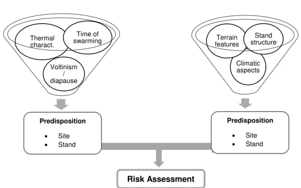
An RA model concerning bark beetle outbreaks can be described with the following component sequence:

Eco-physiologic aspects of Ips typographus Topoclimatic aspects

Figure 1.3 RA structure for the study of bark beetle outbreaks (adapted from Netherer et al. 2004).

According to the theory of predisposition and trigger, the origin of forest damages is based on the combination of favourable spatial and temporal conditions in susceptible forest trees and of different

9

disturbance factors (Führer, 1987). The eco-physiological and topoclimatic aspects have been extensively described and simulated in the past 20 years with the purpose of reducing risk, and consequently the damage that I. typographus outbreaks might cause.

Several of these studies have been performed in Central Europe concerning the factors that are intrinsic to an increase in exposure to an outbreak, their impacts, risk management options, among others. (Schwarzbauer, et al., 2012) (Seidl, et al., 2008) (Kazda & Pichler, 1998). Although the dynamics that lead to an infestation, as with all natural systems, are considerably complex and sensible, compilations and analysis of these studies have allowed to narrow down the main influences behind these outbreaks (Wermelinger, 2004).

For the purposes of this document, the dynamic predisposition assessment system (PAS) from which the main indicators were compiled, for the stand and site used as reference was the one used by Netherer and Nopp-Mayr (2005) in the High Tatra Mountains (Netherer & Nopp-Mayr, 2005). This DPAS considers 17 indicators, divided in the structure already discussed, stand and site-related. It was concluded that the results obtained with this model were in agreement with the hypothesis formulated by the authors, where an increased score of indicator weight, or predisposition, signifies a high probability of damage and that actual infestations or damages, will occur more frequently in high scoring locations (Netherer, et al., 2005).

Another important model that has been developed in recent years for I. typographus development assessment was PHENIPS. This tool allows for the calculation of the microclimatic conditions required for bark beetles seasonal development based on the spatial and temporal simulation of the sites digital elevation model (DEM). After its validation PHENIPS was applied to Kalkalpen National Park in Austria and was found to be able to monitor the actual state of development of the bark beetles at specific stand/tree level levels by explicitly considering effects of regional topography and stand conditions, based on local air and bark temperatures (Baier, et al., 2007).

1.3.1 ArcGIS and MapModels

GIS models that established a connection between decision analysts and computer system design when it comes to geographical data treatment can be highly usefull in risk assessment procedures. The software chosen to perform the analysis on this field was ESRI’s ArcGIS and its former suite, ArcView

a powerful and flexible tool for spatial analysis, data management, mapping and visualization, advanced editing, geocoding and map projections. In 2010 ESRI was found to have more than 40% of the entire GIS marketshare, used by more than 300 000 organizations worldwide (ARC, 2011).

10

in a cloud-based platform, ArcGIS Online (Anon., 2013). This version keeps in with the on-the-move, online network and app-friendly information technology for GIS software, turning map creation, exploration and publishing available for any device that supports it.

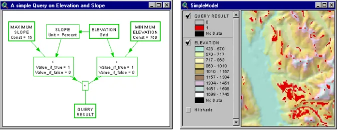
In 2002 a graphical modelling language based on the early ArcView 3.0® was developed at the Institute of Regional Science of the Vienna University of Technology denominated MapModels. It contained a basic function library with various flowchart elements for a range of analysis operations including application of, a highly useful concept for spatial analysis, fuzzy logic (Benedikt, et al., 2002). Its purpose was to act as a Spatial Decision Support System where users with Avenue™ programming skills could extend and/or customize the set according to their preferences (Netherer, et al., 2002). Two of its most relevant features were the built-in fuzzifyfunction that enabled one to construct an ‘award-_{penalty’ score} system based on past literature, and the fact that elements on display were active and could be connected to link and process information within flowcharts.

Figure 1.4 An example of a simple spatial query in MapModels and its respective display, for areas with a maximum slope of 15% and an elevation over 750 meters.

1.3.2 Model Builder

ModelBuilder is an application used to create, edit and manage models through the tools and attributes of ArcMap. These designable models are workflows that string together nodes and variables, where the output of a model or tool is the input of a consequent process (ESRI, 2006). Similarly to the work area of ArcMap, in ModelBuilder when a tool is inserted, a dialog box is prompted and when a file is added it is assigned connectable node.

11

Figure 1.5 Example creation of a raster file with all forest areas from the Stands layer through the workflow basis of ModelBuilder.

Nodes with identical functions or positions have specific colours. Blue coloured oval nodes represent input data, orange nodes represent tools and green oval nodes represent output data. All input or outputs nodes can be configured to be model parameters, thus becoming an essential component to be indicated by the user or extracted from an initial model and used on a following model, as indicated for the Stands inputfile on Fig. 1.5.

Tool nodes can be configured to expose all existing parameters that prompt when the function is selected. This allows a user to customize the conditions in which the tools will operate and output data can be introduced in functions not only as input data but also as function parameters. The nodes that result from each desired parameter to be exposed, is identified with a light blue colour.

A user can also add Environment settings which affect a tool´s result but contrary to other tool parameters, many of these settings when selected do not appear on the dialog box of a tool. A simple example of a use of these settings is applying the Extent Environment setting which allows a certain analysis to be limited to a selected geographic area, defining a new area for the resulting output data. One other valuable feature of ModelBuilder are the iterator tools. These tools grant the possibility to filter or select different operations on files, according to the preferences stated or reference values in which the operations will be based. One of them is the For iterator where interval values for a particular process are assigned, directing different processes for the corresponding input values.

1.3.3 Rosalia Roof Project

12

Apart from temperature, which is a vital condition to the proliferation of a bark beetle population, shortage in water supply due to drought events, or unfavourable site conditions, have also been associated with infestations.

The structure of the evaluation for the roof project was based on the water supply and deficit which may lead to drought stress in terms of tree physiology and ultimately turning them more attractive and less resistant to bark beetle attacks. The tree physiology-related methods used in the project included tree water status, content and potential analysis as well as resin and bark anatomy study. The methods used for bark beetle assessment included monitoring of pheromone traps, their phenology at the site and induced attacks.

The test area consisted of six plots. Two of them were control plots with no cover to allow for the comparison of test conditions with regular functioning conditions in the site. Four plots were fully (2) and semi covered (2), allowing for severity assessment in drought effects. In each of these plots, 3 trees were analysed for the physiological parameters mentioned and subjected to induced bark beetle attacks.

Figure 1.6 Photograph of one of the semi-covered plots (Esteves 2013).

13

Oct-11

Apr-12 Jun-12 Nov-12

Project start and

preparation Plots construction Monitoring

Roof construction & Monitoring under drought stress

Irrigation of fully covered

plots

Figure 1.7 Chronology of the Rosalia Roof Project in 2011 and 2012.

Apr - 13

May – 13 Oct - 13

Oct-14 Project End

Irrigation of fully

covered plots Induced attack by Ips typographus & Monitoring Model establishment

Figure 1.8 Chronology of the Rosalia Roof Project in 2013 and 2014.

The methods used to assess climate and soil parameters were soil hydrological recordings, specifically soil moisture, water potential and temperature, and climate related data: air temperature, precipitation, relative humidity, wind speed and global radiation.

1.4 Objectives

The objectives set out initially to be accomplished focused on the development of a predisposition model on the ArcGIS ModelBuilder software and how its performance concerning the application of data from previous studies into indicators of predisposition of a certain site.

 Develop a structure for the model allowing for a separate analysis, at stand and site level, of hazards resulting from attacks of the bark beetle Ips typographus;

 Integrate the data generated by the Predisposition Assessment Systems as indicator weights;  Ensure flexibility in the model in order to allow for different input conditions according to the

user’s desired scope or choice of procedure;

15

Chapter 2

Materials and Methods

17

2.1 Data and Model Concept

2.1.1 Forest Inventory data

The data used for the development of this model and in particular for the stand-related analysis, originated from an inventory conducted by the ÖBF (Austrian Federal Forests). The OBF is responsible for the monitoring and management of 15% of the Austrian forest area, representing the largest profit-oriented organization in Austria in charge of natural environments. Besides management and reporting services on behalf of the Austrian government, the OBF also promotes public awareness to locals and visitors, as well as partnering with research projects that incorporate their sustainability and conservation objectives (AG, 2013).

The data from the inventory showed that 20% of the tree species identified were spruce, a well-known host for bark beetles especially in areas with frequent windthrow events (Fahse & Heurich, 2011). The stand is located within an altitude range of 400 and 650 meters. The average value of canopy closure was 48.7% and a water supply average of “Moderately Moist”.

The values of water supply for the stand fell within the “Xeric” to “Moderately Moist” categories.

Reported stem damages was minimal, with an inventory scale average value of 0.0023.

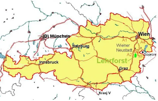
Figure 2.1 Location of the Rosalia Forest referred to as Lehforst (Teaching forest grounds).

18

(Table 3.1). The potential number of I. typographus generations in the study area, which is a main criterion within predisposition assessment, was fixed at two, based on previous modelling activities by use of PHENIPS (Baier, et al., 2007).

The conversion from raw data to adaptable values, was made through conditional functions, statistical analysis and interpretation of the code established by the ÖBF. These codes were linked to the water supply characteristic of each area of the stand, which were identified by a single ObjectID.

The inquiry of the proportion of different species and age class was defined only for the top layer. The parameter age class was only registered for the predominant tree species in the top layer. For the bonity parameter the same principle was applied, where only the predominant tree species, with the highest proportion in the top layer, was evaluated for its yield class.

In the Gleysol parameter, organic wet soils were also taken into account. The scales adopted for these parameters, were adjusted to the DPAS rating system (See section 2.1.6) and later joined with the shapefile, through the same ObjectID.

Table 2.1 Parameters gathered from the inventory of Rosalia Forest stand and classes of value after the process of initial data transformation.

Parameter Classes of value

Forest area Yes/No (1/0)

Proportion of spruce 0 - 100%

Proportion of pine 0 - 100%

Proportion of spruce and fir 0 - 100% Proportion of spruce, pine and fir 0 - 100% Proportion of deciduous trees 0 - 100%

Canopy closure 0.0 - 2.0

Stand age year

Water supply 0 - 7

Bonity 0 - 20

Stem damage 0 - 5

19

Regarding the data on the proportion of species from the stand file, 1.2% of the values were missing or, in some cases, the species label was not mentioned. The problem posed by the missing data was addressed by integrating the values in a category that considered other deciduous tree species so that the proportions that were identified could be integrated into the dataset.

2.1.2 Rosalia Forest Shapefile and DEM

The data in Excel spreadsheet format was joined with the shapefile from the stand area in Rosalia forest through a specific command in ArcMap (See Section 2.2.3). This file allows for the insertion of the data into the corresponding areas, thus granting a possibility to perform a wide variety of study operations, in this case a predisposition assessment.

Concerning GIS file formats, Shapefiles store non-topological geometry and attribute information for the spatial features in a data set and can support point, line and area (polygon) features. The geometry for a feature is stored as a shape comprising a set of vector coordinates. For the purposes of the model, the shapefile contained area data on the stands in polygon shape (ESRI (Environmental Systems Research Institute), 1998).

20

Site related parameters where analysed through the Digital Elevation Model, here after called DEM. This file as well as the DEM, were provided by the Bundesamt für Eich- und Vermessungswesen (BEV), which is a subordinate federal agency of the Federal Ministry of Research and Economy. The main tasks carried out by the BEV are geoinformation surveying and measurement, as well as the calibration of this information. The DEM provided is part of a national geodatabase compiled by the Department of Geomatics, the Austrian Spatial Data Infrastructure.

Spatial data files are an essential part of planning, management and protection of natural systems. As such they provide key information throughout a wide variety of fields of study like agriculture, forestry, homeland security, civil and energy engineering, among others.

DEMs are commonly used in spatial characterization processes in a wide variety of fields of study. DEM data is stored as a point elevation data on either grid, or triangular integrated network (TIN), or as vectorized contours stored in a digital line graph. Grid format is most widely used.

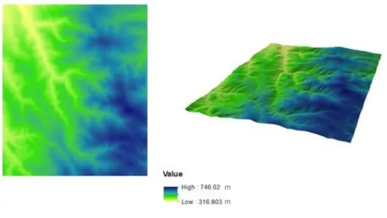
Figure 2.3 TIN (left) and DEM (right) of the Rosalia forest stand area viewed in ArcScene.

The DEM used in this work included the stand site, making it possible to analyse both data sources. The main properties of the DEM (see Table 2.2), were compatible with the shapefile, allowing for spatial and statistical analysis to be carried out in the course of the development of the model.

Table 2.2 DEM properties in ArcMap System.

Property Value

Cell size (X,Y) 10, 10

Format GRID

Pixel Type Floating point Spatial Reference MGI_Transverse_Mercator

21

2.1.3 Structure

Based on a comprehensive review of research papers and expert knowledge (Nopp 1999; Netherer and Nopp-Mayr, 2005), the predisposition of a forest environment to biotic and abiotic damage agents incorporates two main components: the condition of the stand and the characteristics of the site. Following the approach of Speight and Wainhouse (1989) and Berryman (1986) relevant indicators were defined and scored according to their influence on the global predisposition to bark beetle outbreaks within these two components of the Predisposition Assessment System (DPAS).

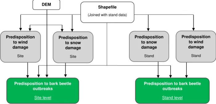
Since the stand and site were analysed separately, the overall predisposition was concomitantly separately developed. Predisposition to snow and wind damage was analysed by discrete assessment systems and results were integrated in the bark beetle PAS. These analyses were performed through submodels having as input the initial datasets and as outputs the indicator results to be ultimately combined. According to the PAS, for site level predisposition, both the DEM and shapefile were also integrated in the final model as the slope and altitude are indicator parameters (Fig. 2.4).

Figure 2.4 Model structure for predisposition assessment for Ips typographus

In Fig. 2.4 a simplified view of the structure of the model is represented, as some of the four submodels, required the preparation of the source files, particularly the DEM. An example of these preparation steps is the Smooth submodel, where ArcGIS tools were applied to even certain surfaces of the DEM, but where no indicators were applied. This ‘smoothed’ DEM provided the new elevation data to be applied in all subsequent models.

Predisposition to wind damage Stand Predisposition to snow damage Stand Predisposition to snow damage Site Predisposition to wind damage Site Shapefile

(Joined with stand data)

DEM

Predisposition to bark beetle outbreaks

Site level

Predisposition to bark beetle outbreaks

22

2.1.4 PAS approach

The values established by PAS resulted from the product between relative scores within an indicator and the relative importance of an indicator (weighting). The resulting values from this product are the relative weights and consequently the scores for each indicator. The break values for which a defined score is assigned, is denominated as fuzzy number.

Figure 2.5 Graphical display of the fuzzy number grading in the Slope Gradient indicator regarding predisposition to wind damage on site level.

Upon the confirmation of the relative scores, one can estimate a set of values corresponding to their score using fuzzy numbers logic. In Fig. 2.5 the slope gradient values are graded within a [0, 0.40] interval. This principle was applied to the parameters that were defined within the scope of the system and ultimately summed, with their respective weight. Depending on the stand data, the indicators were either continuously or discretely weighed.

2.1.5 Data join

Before proceeding with the model construction in ModelBuilder, two of the original datasets, the shapefile and excel data from the forest inventory needed to be adapted and joined afterwards joined. As mentioned in Section 2.1.2., the stands data contained in the excel file were fitted to the indicator classes needed to rate the areas predisposition to wind and storm damage and subsequently for bark beetle outbreaks.

The function used to associate this data with the areas that they describe was the Join command of ArcMap. Joining data commands are typically used to append the fields of one table to those of another

0.00 0.10 0.20 0.30 0.40 0.50

0 20 40 60 80 100

Slope gradient (%)

Sc

or

23

through an attribute or field common to both tables. In this case the common field would be the identification area number, ObjectID.

Figure 2.6 Join command dialog box in ArcMap prompted from the shapefile, being Sheet1 the excel sheet to be joined with the table of the shape file.

The resulting output file from this command is the shapefile containing all the necessary information for the consequent model operations, remaining in FLOAT format.

2.1.6 Indicators: stand and site level

The indicator values for stand level of the PAS, regarding wind, snow and bark beetle damage, related to four parameter categories: tree species composition, structure, vitality and predisposition to wind and snow damages (Table 2.3 and Table 2.4).

Level Parameter Criterion

Stand Species composition Proportion of spruce (%)

24

Table 2.3 List of all PAS indicators on stand level.

Table 2.4 List of all PAS indicators on site level.

Structure Stand Age - Alterklasse (years) Canopy closure (%)

Phase of stand development (years)

Stand Edges Vitality Stem damages Predisposition to Wind Damage (%)

Snow Damage (%)

Level Parameter Criterion Site Generation factor Temperature

Soil Hydrology Gleysol

Bonity (Productivity)

Terrain Altitude (m) Slope (%) Morphology

25

2.2 Indicator scoring tools

2.2.1 Reclassify

In order to incorporate the values of each indicator into the model, a transformation of the scale of the initial data or of the output results of the submodel was needed. ArcGIS has several tools that allow to manage the data according to the objective of the user. Toolboxes such as Spatial Analyst, Spatial Statistics, Analysis, 3D Analyst, Data Management, among others provide, for example tools that transform value intervals and classes on data, calculate new fields and data attributes or join fields from different files.

Another function that allows for the transform input data into new values, according to the PAS is the Reclassify tool from the Spatial Analyst toolbox. With Reclassify the user selects the target-reclass field and constructs its reclassification from old values to new values. Although it is a considerably flexible tool in terms of freedom to choose reclassification methods and intervals, this tool is restrictive when trying to reclass continuous data and still maintain its continuous attribute.

A common example of an application of this tool is land use categorization. For example, using as an input raster data water availability, ranked from 1 to 20, 20 being a perfectly water supplied area, it would be possible establish the land uses for each area, irrespectively of the planning purpose - agricultural, forestry, or urban, with new classes, from 1 to 5 (Fig2.7).

Figure 2.7 Land use reclassification example through the Reclassify tool.

26

2.2.2 Fuzzy Membership

Another tool that enables a user to perform an indicator-like ranking of results and translating them into a fuzzy set is the Fuzzy Membership function from the Spatial Analyst toolbox. Fuzzy sets are defined by assigning to every object a membership grade to the whole that represents a concept

This tool transforms the data from the input raster into a 0 to 1 range, indicating the strength of a membership within its dataset with 1 being absolutely in the set. This strength evaluation can be based on several fuzzification algorithms. Each one of the algorithms available in the Fuzzy Membership tool in ArcGIS defines a continuous function and each function captures a different type of transformation (ESRI, 2013).

Table 2.5 Description of the function in Fuzzy Membership tool (Adapted from ArcGIS Resource Center overview of fuzzy classes).

An important aspect of this tool is that when the input are continuous values, they remain continuous i.e. the only aspect that is modified is the range in which they are represented. This property is the result of the application of a function instead of combining several values into one single category, which is the method that the Reclassify tool applies.

Membership Function Description

Gaussian Membership defined through a Gaussian or normal distribution based on a midpoint indicated by the user with a defined spread decreasing to zero.

Large Large input values have a membership closer to 1. The user provides de midpoint, which is assigned a membership of 0.5, with a defined spread.

Linear

Membership defined by a linear transformation between the user-specified minimum value, which gets an attributed membership of 0, and maximum value, which is assigned a membership of 1.

MSLarge Membership defined through a function based on the mean and standard deviation, with larger values having a membership closer to 1.

MSSmall Membership defined through a function based on the mean and standard deviation, with the smaller values having a membership closer to 1.

Near Membership defined through a function around a specific value which is provided by the user as well as a specific spread decreasing to zero.

27

Figure 2.8 Linear fuzzy membership with 30 as the minimum value and 70 as the maximum value.

The approach carried out with a linear fuzzy membership indicates that a dataset, within a 0 to 1 range, receives a membership value based on a linear scale with a large input value being assigned a greater possibility, i.e. is placed closer to 1. However, this presents some operational issues in particular for more complex membership studies, for alternative membership ranges, among other conditions that would require a more customizable tool.

2.2.3 Linear and Sine Fuzzify Function

The use of Fuzzy Membership proved to have several limitations and uncovered the need of a more customizable tool. A fuzzify function was thus developed, allowing the user to fix the start and ending points of the membership ranges, as well as to select the type of function on which to base the membership.

ArcGIS has a wide variety of tools, besides those mentioned in Section 2.2.1 and 2.2.2, and script functionalities, but still the editing of the tools is still restricted. For the desired purposes of the PAS, a hybrid tool for ArcMap was developed which would integrate fuzzy membership principles and support the customizing and management of the properties of the analysis.

28

Figure 2.9 Raster calculator dialog box where a conditional (Con) function is used. MeanDEM as input Layer and map algebra expression where the desired operation is to divide all values between 100 and 600 inclusive of the

input file by 10. All other values are assigned a value of 0.

By taking advantage of the third section of this function, which refers to the values that are not included in the first expression, a user can extend the calculation substantially. If we consider the example given in Fig. 2.9, in order to perform a different calculation for altitudes above 600 meters, it is only necessary to include another conditional function and the corresponding algebra expression in the third section of the first conditional function (Equation 2).

Equation 2.1 Con( (“%MeanDEM%” > 100) & (“%MeanDEM%” <= 600) , (“%MeanDEM%” / 10) , Con ( (“%MeanDEM%” > 600), 2 , 0 ) ) )

In Equation 2.1 for values above 600 meters, considering the data from the file “MeanDEM”, the value

2 is attributed. For values that do not fall within the range of the analysis, from 100 to infinity, the value 0 is attributed. This feature enables the user to diversify its analysis, apply different methods to the data range in an efficient way by resorting to just one tool.

This is a key aspect to be considered for the construction of indicators that simultaneously do not behave linearly and do not fall within the 0 – 1 scale, both of which preclude the use of the Fuzzy Membership tool. A possible way to include this tool in the construction of the indicator is to perform an initial reclassification of the data, through the Reclassify tool, and then apply the Fuzzy Membership function.

29

Considering the advantages and disadvantages of each calculation process, it was decided that integrating equations that would represent the behaviour of the indicators for each interval in a single tool would be the most efficient and straightforward procedure to integrate the PAS into the model. The basis for these calculations was the Raster Calculator tool and the input are the values prepared in Excel and the Layer file to which the indicators will be applied.

Firstly, in order to describe a linear trend one must calculate its slope and interception on the y-axis. A slope constitutes the rate at which an ordinate of a point of a line on a coordinate plane changes with respect to a change in the abscissa. In an indicator construction scope this represents the quotient between two ranges: parameter values and corresponding indicator scores.

Knowing the slope, the y-axis interception value is given by inserting any corresponding values in the equation.

Equation 2.2

Using Equation2.2as a basis the function for both negative and positive linear slope indicator trends is obtained. When the objective is to rank the score of a parameter, the fuzzy logic should be applied and the border fuzzy numbers used as direct input for each trend. In sequence the equation obtained is then inserted it in the Raster Calculator tool. This methodology enables the data to be calculated and scored while maintaining their continuous attribute.

The use of this type of logic can be exemplified by considering a continuous dataset file that will be the object of an indicator score analysis. This indicator will have two trend scoring patterns with the following scores:

Table 2.6 Scoring example table for a non-linear trend indicator. V1 > V3 >V2 results into a decreasing trend from V1 to V2 and in an increasing trend from V2 to V3.

The resulting two equations (Equation 2.3 and Equation 2.4) based on Eq. 2.2 and correspondent graphics that describes the trends and border score values are the following:

Criterion Indicator Score

C ≤ x1 V1

x2 V2

≥ x3 V3

Slope

𝑦(𝑥) =

𝑦

_𝑥

2

− 𝑦

1

30

Equation 2.3

v

_i

(x) =

v2−v1

x2−x1

∗ (x − x

2

) + v

2

and

Equation 2.4

v

_ii

(x) =

v3−v2

x3−x2

∗ (x − x

3

) + v

3

In both equations, x represents the input data value for which a score value will be calculated, being all other values parameters that refer to the slope and y-axis, in this case v-axis, of the indicator linear function.

Figure 2.10 Example of a non-linear indicator trend.

If the calculation of more trends and respective indicator values is needed, the same logic will be extended and integrated in the raster calculator tool. For the example presented above with the values from Table 2.6 the Map algebra that would incorporate the Raster Calculator tool of ArcMap is the following, for a given file with the name ‘Data’:

With the introduction of a second conditional clause (Con), the values from x2 and on, are affected by the second linear equation, thus following the scores previously established in the PAS.

The second category of function that was used in the construction of this model was the sine function. This function is one of the basic functions encountered in trigonometry, the others being cosecant, cosine, cotangent, secant and tangent. The sine function has a period of 2_𝜋.

31

As this category of function behaves as a wave, a mathematical curve, it is often applied in physics, signal processing and many other fields. The most basic form of a sinus function, as a function of time is the following:

Equation 2.5

y(t) = A sin(ωt + φ)



A

–Wave amplitude, the peak deviation of the function from zero;



_𝜔

(2

_{𝜋 ∗}

f

)

–

Angular frequency, the change of rate of the function argument;



_𝜑

–

The phase, specifies where the oscillation is at t = 0.

This initial equation has to be adapted to a format allowing to incorporate values from the PAS and to apply them to the range of values of a map. Hence reformulation of this equation was conducted where the initial and final fuzzy numbers, and the initial point of the function considering a sinus-shaped function, are provided by the user.

Equation 2.6

f(x) = |f

₁

− f

₂

| ∗ sin ((

π

0.5

) ∗ (x + x

i

)) + f

1

After the scoring range is set, a sine function can be constructed that behaves in a smoother manner considering a change in trend signal. A clear example for indicator function construction would be an indicator with a rank between 0.25 and 0.75, for values between 0 and 6, with the following behaviour:

Equation 2.7 f(x) =

{

0.25 , x ≤ 1

0.25 ∗ (x − 2) + 0.5, 1 < x ≤ 2

0.25 ∗ sin ((_0.5∗4π ) ∗ (x − 2)) + 0.5 , 2 < x ≤ 4

− 0.25 ∗ (x − 5) + 0.25, 4 < x ≤ 5

0.25 , x > 5

32

of the scoring range, a sinus trend is applied. The goal in implementing this trend is to simulate a more gradual and less abrupt change in slope.

Figure 2.11 Graphical representation of equation 2.7 with linear trends for a hypothetical scoring of features with values ranging from 0 to 6

Figure 2.12 Graphical representation of equation 2.7 with linear and sinus trends for an hypothetical scoring of features with values ranging from 0 to 6.

33

2.3 Preparatory Models

2.3.1 Data Preparation Models

Smooth Model

The initial step in developing the predisposition model would be to adjust the initial DEM to a smoother surface. The importance of undergoing this process resides in the adjustment of values that might misrepresent the area, values that suddenly change or cells with lack of data. All these occurrences potentially influence data processing flow or process data in an imprecise or misrepresentative way.

Figure 2.13 Workflow of the Smooth Model. The output raster DEM S signalled with a P indicating it as a Model Parameter.

The tool used to adjust the DEM was Focal Statistics, from the Spatial Analyst toolbox. This tool calculates for each input cell location a statistic of the values within a specified neighbourhood around it. The neighbourhood classes that the tool provides are Annulus, Circle, Rectangle, Wedge, Irregular and Weight and the statistics units can either be cell or map based. The type of statistics applied to the file was Mean, for a circle neighbourhood and cell size of 3 units.

The output file be like the input Elevation file, denominated DEM S for the consequent models, making this the first step after the joining of the excel data with the shapefile (Section 3.2.1).

P

34

Figure 2.14 Output rastermap from the Smooth Model.

Aspect Model

From previous analysis on the Rosalia forest, the value of aperture angle was 270° and orientation was 315°. The value for orientation referred to the predominant wind direction observed in the site during past studies. As wind is an important component of the PAS, it was essential to develop an Aspect-based raster file where the slopes that had the same orientation as a certain wind direction would be defined.

35

With the previous value of orientation of 315° one can adapt the original range of values from the Aspect tool using map algebra. The Adjust submodel performs this range adaptation and prepares it for the Aspect model.

Figure 2.15 Output rastermap from the Adjust submodel.

36

Two linear fuzzy membership functions were applied considering the previously stated aperture angle and orientation values. One of the fuzzy membership function ranked from 0 to 1 the output rastermap from the Adjust model in an increasing trend from 0º to 180º and the second ranked in a decreasing trend from 180º to 360º. The application of this procedure means that the same value of 0.5 was attributed for a slope with a direction of 270º or 90º, in reference to the 315º orientation angle.

Figure 2.16 Workflow of the Aspect Model with theAdjust submodel integrated.

37

Low-Middle-High Slopes and Range submodel

Slope characterization for the Rosalia forest is a key component of the predisposition assessment. This terrain feature is the first derivative of a surface and has both magnitude and direction. It can be derived from the TIN or DEM using tools that GIS software, such as ArcGIS provide (Li, et al., 2010). In the Low-Middle-High Slope Model, the goal was to describe the slopes into 3 categories, each with their corresponding interval.

The calculation would be based on two separate procedures. One would be to establish an euclidean range for areas characterized by water flow from the prepared DEM and the other to identify and also establish and Euclidean range for convex surface areas. The final step consists in dividing the resulting rastermaps and applying a Range Model where the low, middle and high denominated slopes can be identified.

For the first procedure, several spatial analyst tools were used. In the first calculation the Flow Direction tool is applied. With this tool, one creates a raster of flow direction from each cell to its steepest downslope neighbour, thus providing useful hydrological information that would serve as input for the Flow Accumulation tool. Here the values are evaluated to describe a flow pattern as the accumulated weight of all cells flow into each downward sloping cell in the output raster.

Based on past research, specifically early model constructions with MapModels (See section 1.3.1) it was established that a threshold of 1000 flow accumulation cell values would represent a considerable water flow. With this value, a conditional tool (Con) was implemented, assigning a value of 1 to all cell values above or equal to the pre-established 1000 accumulation value and 0 otherwise. The result of this calculation produced a raster file with all designated water flows for the Rosalia forest.

This file is the input for the Euclidean Distance tool. This tool calculates for each cell, the distance to the closest source and a value of zero is appointed to a legitimate source. The aim of this process is to construct a range of values representing the relative proximity to water flow-supportable terrain. The

output file would be denominated “riverseucl”.

Simultaneously the DEM file was also analysed for convex-shaped terrain. The first tool to be used should be the Focal Statistics with a neighbourhood of 6 cells, larger than the one used in the Smooth Model (see section 2.3.1) in order to expand the analysis range further and include possible outlier terrain surfaces. The following tool applied should be a Curvature tool where the curvature of a surface is calculated on a cell-by-cell basis, assigning a positive value for convex surfaces, 0 for plain surfaces and negative values for concave surfaces.

Similarly to the process conducted to obtain a Euclidean distance raster file of the previously threshold for the defined river areas, a threshold for convex areas was defined using a conditional tool (Con). The threshold level selected was 0.3 so that only distinct convex surfaces would be included.

38

this tool represents the relative distance from convex area to which a value of zero will be asigned. With both Euclidean distance tool-originated files, a quocient between the riverseucl file and a file corresponding to the sum of both the riverseucl and conveucl was applied. The output file from this division represents the normalized values of river-like surfaces, in this case low slopes, from all convex surfaces. Instead of analysing the slopes in terms of percentage or grade rise, with this file one yields a range of slopes with the terrains that result from the riverseucl as referrence.

Figure 2.17 Workflow of the Low-Middle-High Slopes model and the integration of the Range Model. The output files to be used on subsequent submodels signalled with the Model Parameter symbol (P).

39

The final step consists in defining the range for low, middle or high slopes. This procedure was conducted through a mask submodel denominated Range (Annex A). This submodel has as prerequisite parameters, besides an input raster file, a centre value and a range value.

All raster values above a threshold of centre value plus range value were designated as high slopes, all values under a threshold of centre value minus range value were designated as low slopes and all in between middle slopes. With this last step the user obtains a map where low, middle and high slopes are differentiated according to specific threshold values using as reference the surfaces designated as rivers.