1
David João Nunes Palma
Licenciatura em Engenharia Electrotécnica e de Computadores
Design of Future Distribution Grids
Dissertação para obtenção do Grau de Mestre em Engenharia Electrotécnica e de Computadores
Orientador: Prof. João Francisco Alves Martins Co-orientador: Dipl. Ing. Jörg Dickert
Júri:
Presidente: Prof. Doutora Anabela Gonçalves Pronto Vogal(ais): Dipl. Ing. Jörg Dickert (Co-orientador) Prof. Doutor Duarte de Mesquita e Sousa (Arguente) Prof. Doutor(a) João Francisco Alves Martins (Orientador) Prof. Doutor João Miguel Murta Pina (Arguente)
3
Statement
This thesis does not contain material previously published or written by another person, except where due reference is made. The material contained in this work has not been previously submitted to meet the requirements for an award at this or any other higher education institute.
__________________________________________
Author’s signature
_________________
4
Dedico esta tese:
À minha mãe e à minha família
À minha namorada
5
i.
Resumo
O presente trabalho introduz o conceito de controlo de tensão em sistemas de distribuição de energia, que incluam geração distribuída e veículos eléctricos. O impacto da geração distribuída e dos veículos eléctricos no abastecimento de tensão será avaliado. Por um lado a geração distribuída providencia mais potência para o sistema, o que pode causar a inversão do fluxo de potência e um aumento no nível de tensão na sua proximidade quando a carga é reduzida. Por outro lado, os veículos eléctricos representam uma carga adicional em sistemas de distribuição, levando ao aumento da procura de mais potência da rede, e da queda de tensão ao longo dos ramos de distribuição do sistema. Ambos poderão causar problemas de tensão no abastecimento de energia, caso não seja implementado um sistema de controlo de tensão. Dispositivos, tais como o transformador equipado com tomadas comutáveis, ou o regulador automático de tensão, que não eram elementos essenciais no passado, são hoje soluções importantes para a regulação de tensão.
Neste projecto diversas soluções para o controlo de tensão são analisadas, tanto de um ponto de vista técnico como económico. No geral, os resultados mostram que diferentes estratégias conduzem a resultados diferentes, e algumas soluções demonstram ser melhores que outras no controlo de tensão. No momento de decidir qual a estratégia a implementar, de forma a obter uma solução adequada para um determinado sistema, é necessário ter sempre em conta a capacidade dos condutores, os limites técnicos de cada dispositivo e os custos associados aos mesmos.
6
ii.
Abstract
This work presents the concept of voltage control in power distribution systems with distributed generation and electric vehicles penetration. The impact of DG and EV in the voltage supply is investigated. DG provides more power into the system, which can cause the inversion of the load flow and an increase in the voltage supply when the demand is low. EVs on the other hand are additional load in distribution systems, increasing power demand and voltage drop. Both might be a cause of voltage problems in the power supply, when no voltage control is applied. Devices such as the tap-changer transformer or the voltage regulator which were not essential in the past are now important solutions to solve voltage variation issues. In this work, several different solutions for voltage control are analyzed, both technically and economically.
Overall, the results show that different strategies have different outcomes, and some solutions provide better voltage control than others. In order to have a proper solution for a system, when choosing a control strategy, it is necessary to always take into account the cable ampacity, the technical limits of each device and the costs associated with it.
7
iii.
Acknowledgements
This work has been carried out, during 6 months, from 3 December 2012 to 3 June 2013, at the Institute of Electrical Power Systems and High Voltage Engineering (IEEH) of the Technical University of Dresden (TUD), in Germany.
I would like to express my gratitude to my supervisor, Mr. Jörg Dickert from the IEEH, who, through his guidance, has made possible the accomplishment of this work. My gratitude also goes to Professor João Martins from the Department of Electrical and Computer Engineering (DEE) of Faculty of Sciences and Technology – New University of Lisbon (FCT-UNL), my home university, for being available to accompanying this work.
I would also like to express my gratitude to Professor Peter Schegner from the IEEH, for giving me the opportunity to finish my master degree at the TUD, which was an honor for me.
8
Contents
I. RESUMO ... 5
II. ABSTRACT ... 6
III. ACKNOWLEDGEMENTS ... 7
IV. LIST OF FIGURES ... 10
V. LIST OF TABLES ... 13
VI. LIST OF EQUATIONS ... 14
VII. LIST OF ABBREVIATIONS ... 15
CHAPTER 1 ... 16
INTRODUCTION ... 16
1.1 MOTIVATION ... 16
1.1 POWER DISTRIBUTION:THE PAST, THE PRESENT AND THE FUTURE ... 17
1.2 EUROPEAN SMART GRID R&D ... 19
1.3 OBJECTIVES ... 20
CHAPTER 2 ... 21
POWER DISTRIBUTION SYSTEM ... 21
2.1 INTRODUCTION ... 21
2.2 THE PRESENT DISTRIBUTION SYSTEM ... 23
2.2.1 Structure ... 23
2.2.2 Components ... 24
2.2.3 Requirements ... 25
2.3 THE LOAD ... 25
2.3.1 Load Class ... 26
2.3.2 An Introduction to Load Modeling ... 30
2.3.3 Load Behavior ... 32
2.3.4 Load Demand ... 37
2.4 FUTURE POSSIBILITIES FOR DISTRIBUTION ... 41
2.4.1 DC Distribution ... 41
2.4.2 Single vs. Two vs. Three-phase system ... 45
2.4.3 Smart Metering System ... 48
2.4.4 Voltage Level Used ... 48
2.4.5 Demand Side Management... 49
2.4.6 Conductor upgrades ... 49
2.4.7 Energy Storage ... 49
2.4.8 FACTS in distribution ... 49
2.5 CASE STUDY ... 52
2.6 CONCLUSIONS ... 57
CHAPTER 3 ... 58
VOLTAGE CONTROL IN DISTRIBUTION SYSTEMS ... 58
3.1 INTRODUCTION ... 58
3.2 VOLTAGE DROP AND ITS IMPACT ON DISTRIBUTION ... 59
3.3 VOLTAGE CONTROL ... 63
9
3.3.2 Voltage Regulator ... 69
3.3.3 Reactive power ... 72
3.3.4 Load Transfer ... 75
3.4 VOLTAGE CONTROL IN THE PRESENCE OF DISTRIBUTED GENERATION ... 76
3.4.1 Overview of distributed generation technology ... 76
3.4.2 Intermittent Inversion of the Power Flow and its Impact on Distribution ... 77
3.5 VOLTAGE CONTROL IN THE PRESENCE OF FUTURE LOADS ... 78
3.5.1 Electric Vehicles and Electric Heat Pumps in Distribution Systems ... 79
3.5.2 Future possibilities for EVs in Distribution Systems ... 80
3.6 VOLTAGE CONTROL IN DCDISTRIBUTION SYSTEMS ... 80
3.6.1 Low Voltage Direct Current ... 83
3.7 CASE STUDY ... 85
3.7.1 Results ... 90
3.7.2 Overall Voltage Regulation Required for Each Solution ... 126
3.8 ECONOMIC ANALYSIS OF DIFFERENT SOLUTIONS ... 128
3.9 CONCLUSIONS ... 135
CHAPTER 4 ... 136
4.1 CONCLUSIONS AND FUTURE WORK ... 136
10
iv.
List of figures
Figure 1 – A typical power grid ... 17
Figure 2 – An actual power grid with distributed generation ... 18
Figure 3 – A vision of the future power grid ... 19
Figure 4 – Primary Distribution System ... 23
Figure 5 – European Primary System ... 23
Figure 6 – Residential demand by load type ... 34
Figure 7 – Residential demand by load group ... 34
Figure 8 – Typical demand of common appliances per day ... 36
Figure 9 – Load vs. frequency of use per year for several appliances ... 36
Figure 10 – Variations of exponential and ZIP load model coefficients during a typical spring day ... 37
Figure 11 – Typical load profile for residential loads ... 38
Figure 12 – Typical load profile for commercial loads ... 38
Figure 13 – Typical load profile for small to medium industry ... 38
Figure 14 – Typical load profile for large industry ... 39
Figure 15 – Coincidence factor as a function of the number of customers ... 40
Figure 16 – Typical AC UPS system... 43
Figure 17 – A DC UPS system ... 44
Figure 18 – Relation between rate of occurrence and voltage level for single, two and three-phase systems ... 46
Figure 19 – Number of phases associated with a voltage drop to 85% ... 46
Figure 20 – Number of phases associated with a voltage drop to 20% ... 46
Figure 21 – Smart meter ... 48
Figure 22 – Types of series compensation using FACTS ... 50
Figure 23 – Types of shunt compensation using FACTS ... 51
Figure 24 – Different topologies for static var compensators ... 51
Figure 25 – Single radial distribution system ... 52
Figure 26 – Voltage profile for each standard load model ... 54
Figure 27 – Voltage difference between each standard load model ... 55
Figure 28 – Short line equivalent circuit ... 59
Figure 29 - Voltage diagram using vectors ... 60
Figure 30 – Transformer equipped with OLTC ... 64
Figure 31 – On-Load Reactor ... 64
Figure 32 – On-Load Resistor ... 65
Figure 33 – Electronically-assisted version of on-load resistor (b) arrangement ... 66
Figure 34 – An improved version of the electronically-assisted OLTC ... 67
Figure 35 – Substation Voltage Regulators ... 69
Figure 36 – Basic voltage regulation using an autotransformer ... 69
Figure 37 – Modern, 32-step, single-phase voltage regulator ... 69
Figure 38 – Siemens three-phase voltage regulator ... 70
Figure 39 – LDC circuit ... 70
Figure 40 – Comparison between absence and presence of LDC control ... 71
Figure 41 – Total reactive power compensation vs. distance along the feeder for different types of shunt capacitors ... 73
Figure 42 – Static transfer switch ... 76
Figure 43 – A DC distribution system ... 80
Figure 44 – An AC/DC converter using diodes ... 81
Figure 45 – A diode AC/DC converter with PFC ... 81
11
Figure 47 – Three-level VSC ... 82
Figure 48 – VSC with buck ... 82
Figure 49 – LVDC Distribution District ... 83
Figure 50 – Link LVDC Distribution System ... 83
Figure 51 – Bipolar LVDC system ... 84
Figure 52 – Unipolar LVDC system ... 84
Figure 53 – DC Distribution Power vs. Distance ... 84
Figure 54 – System 1 (residential) ... 89
Figure 55 – System 2 (commercial)... 89
Figure 56 – System 3 (industrial) ... 89
Figure 57 – High demand, low generation case: voltage level per node without direct voltage regulation ... 90
Figure 58 – Low demand, high generation case: voltage level per node without direct voltage regulation ... 91
Figure 59 – High demand, low generation case: overload level per feeder without voltage regulation ... 91
Figure 60 – Low demand w/ high generation: overload level per feeder without voltage regulation ... 92
Figure 61 – System 1 using voltage regulators in series (case 1) ... 94
Figure 62 – High demand, low generation, no EV charging: node voltage using voltage regulators in series ... 95
Figure 63 – Low demand, high generation, no EV charging: node voltage using voltage regulators in series ... 95
Figure 64 – Low demand, high generation, EV charging: node voltage using voltage regulators in series ... 96
Figure 65 – High demand, low DG, no EV charging: feeder load using voltage regulators in series ... 96
Figure 66 – Low demand, high DG, no EV charging: feeder load using voltage regulators in series ... 97
Figure 67 – Low demand, high DG, EV charging: feeder load using voltage regulators in series ... 97
Figure 68 – System 1 using voltage regulators in parallel (case 2) ... 98
Figure 69 – High demand, low DG, no EV charging: voltage levels using voltage regulators in parallel ... 99
Figure 70 – Low demand, high DG, no EV charging: voltage levels using voltage regulators in parallel ... 99
Figure 71 – Low demand, high DG, EV charging: voltage levels using voltage regulators in parallel ... 99
Figure 72 – High demand, low DG, no EV charging: feeder load using voltage regulators in parallel ... 100
Figure 73 – Low demand, high DG, no EV charging: feeder load using voltage regulators in parallel ... 100
Figure 74 – Low demand, high DG, EV charging: feeder load using voltage regulators in parallel ... 100
Figure 75 – High demand, EV charging, low DG: voltage level using OLTC in substation 102 Figure 76 – Low demand, no EV charging, high DG: voltage level using OLTC in substation ... 103
Figure 77 – High demand, EV charging, low DG: feeder load using OLTC in substation.. 103
Figure 78 – Low demand, no EV charging, high DG: feeder load using OLTC in substation ... 103
Figure 79 – High demand, low DG: voltage level using ±10% regulation ... 104
Figure 80 – High demand, low DG: voltage level using ±20% regulation ... 104
12
Figure 82 – High demand, low DG: voltage level using ESUs ... 106
Figure 83 – Low demand, high DG: voltage level using ESUs ... 106
Figure 84 – System 1 with a higher AC voltage supply ... 108
Figure 85 – High Demand, low Generation: voltage level using higher supply voltage ... 109
Figure 86 – Low Demand, high Generation: voltage level using higher supply voltage ... 109
Figure 87 – High demand, low generation: feeder load using higher supply voltage ... 109
Figure 88 – Low demand, high generation: feeder load using higher supply voltage ... 110
Figure 89 – System 1 with DC distribution ... 112
Figure 90 – High Demand, Low Generation: voltage level using a LVDC ... 113
Figure 91 – Low Demand, High Generation: voltage level using a LVDC ... 113
Figure 92 – voltage level control using EVs discharging at 5kWh ... 115
Figure 93 – voltage level control using EVs discharging at 15kWh ... 115
Figure 94 – Low demand, high generation: voltage level control using EVs ... 115
Figure 95 – Feeder load using EVs discharging at 5kWh ... 116
Figure 96 – Feeder load using EVs discharging at 15kWh ... 116
Figure 97 – Feeder load using EVs charging at 20kWh ... 116
Figure 98 – High demand, high generation case (sunny day): voltage level per node without direct voltage regulation ... 119
Figure 99 – High demand, low generation case (cloudy day): voltage level per node without direct voltage regulation ... 119
Figure 100 – Low demand, high generation case: voltage level per node without direct voltage regulation ... 120
Figure 101 – Voltage control using fuel cells: high and low demand cases ... 120
Figure 102 – Feeder load using fuel cells: high and low demand cases ... 121
Figure 103 –Using fuel cells to supply groups of EVs ... 121
Figure 104 – System 2 using ESUs ... 122
Figure 105 – Proposed coordinated control using ESUs, substation, nodes and DG ... 122
Figure 106 – Voltage control using ESUs: normal, high and low demand cases... 122
Figure 107 – System 3 (industrial): low demand case, without any voltage regulation ... 123
Figure 108 – System 3 (industrial): increasing demand and generation case, without any voltage regulation ... 124
Figure 109 – System 3 (industrial): voltage level during high demand, high DG generation and power factor correction ... 124
Figure 110 – System 3 (industrial): feeder load during low demand, high DG generation (wind) and no compensation ... 125
Figure 111 – System 3 (industrial): feeder load during an increasing demand and DG generation (fuel cells) and no compensation (first case) ... 125
Figure 112 – System 3 (industrial): feeder load during low demand, low DG generation and compensation active (second case) ... 125
Figure 113 – System 3 (industrial) normal conditions: high demand, high DG generation (fuel cells) and compensation active ... 126
Figure 114 – Voltage regulation required for different solutions ... 127
Figure 115 – Feeder load for different solutions ... 127
13
v.
List of tables
Table 1 – Typical brown goods ... 26
Table 2 – Typical white goods ... 27
Table 3 – Typical small appliances ... 27
Table 4 – Typical lighting ... 27
Table 5 – Types of residential customers ... 28
Table 6 – Standard load models ... 30
Table 7 – Example of a typical household appliances and their load model ... 33
Table 8 – Daily use and utilization per year of common household appliances ... 35
Table 9 – Coincidence factors and power demand per customer type ... 40
Table 10 – Simulation data ... 52
Table 11 – Comparison between constant power and constant current model ... 53
Table 12 – Comparison between constant power and constant impedance model ... 53
Table 13 – Comparison between constant current and constant impedance model ... 54
Table 14 – Voltage regulation required for each standard load model ... 55
Table 15 – Total load demand, power losses and power ratio for each standard load model 56 Table 16 – Comparison between different AC/DC interfaces ... 83
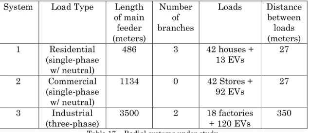
Table 17 – Radial systems under study... 85
Table 18 – Load types under study ... 85
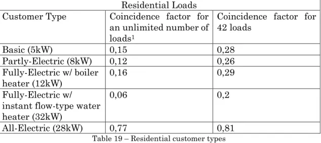
Table 19 – Residential customer types ... 86
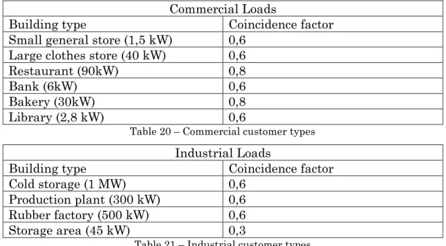
Table 20 – Commercial customer types ... 87
Table 21 – Industrial customer types ... 87
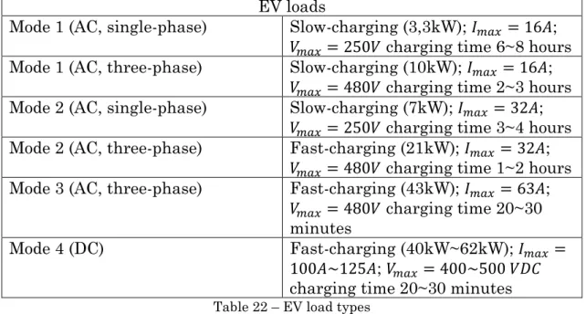
Table 22 – EV load types ... 88
Table 23 –Simulation data ... 88
Table 24 – Simulation data for voltage regulators on system 3 ... 93
Table 25 – Technical data for the battery bank ... 105
Table 26 – ESU: voltage regulation required for system 1 (residential) ... 106
Table 27 – ESUs: voltage regulation required for system 2 (commercial) ... 106
Table 28 – ESUs: voltage regulation required for system 3 (industrial)... 107
Table 29 – Technical data for increased AC voltage simulation ... 108
Table 30 – Comparison: voltage regulation required before/after applying a higher AC voltage supply ... 110
Table 31 – Technical data for the DC simulation ... 111
Table 32 – Technical data and assumptions for the V2G simulation... 114
14
vi.
List of equations
1 ... 25
2 ... 25
3 ... 25
4 ... 30
5 ... 30
6 ... 30
7 ... 30
8 ... 30
9 ... 31
10 ... 31
11 ... 39
12 ... 39
13 ... 40
14 ... 40
15 ... 55
16 ... 59
17 ... 59
18 ... 60
19 ... 60
20 ... 60
21 ... 60
22 ... 61
23 ... 72
24 ... 72
25 ... 72
26 ... 77
15
vii.
List of abbreviations
DG – Distributed Generation/Distributed Generator LV – Low Voltage
MV – Medium Voltage HV – High Voltage
HVAC – Heating, Ventilation and Air-Conditioner VR – Voltage Regulator
AVR – Automatic Voltage Regulator OLTC – On Load Tap Changer ESU – Energy Storage Unit EV – Electric Vehicle
LVDC – Low Voltage Direct Current HVDC – High Voltage Direct Current AC – Alternate Current
DC – Direct Current
SC – Synchronous Condenser G2V – Grid to Vehicle
V2G – Vehicle to Grid
VRU – Voltage Regulation Unit
16
Chapter 1
Introduction
This chapter is a general introduction to the work, “Design of Future Distribution Grids”. It starts with a brief overview of the power grid concept, how it has been
developing from its earlier stages up to the present and how it is expected to change in the near future, to deal with the energy demand, improve itself and become the much spoken smart grid concept. The integration of distributed generation and the expected increase of loads – trough the development of electric cars and heat pumps - in distribution systems are major factors for the power grid need of change and both are then explored further.
1.1
Motivation
17
1.1
Power Distribution: The Past, the
Present and the Future
Since it was invented in the nineteen century, the electric power system, also known as the power grid, has been performing a decisive role regarding the social, technological and economic development of every nation. In fact, its creation changed many aspects about life on earth; it supported innumerous technological advances in many scientific areas; it is also related to each nation with its own economy, directly affecting and influencing it, by becoming a piece of the global market in order to sell its primary good, the electric energy. It shaped the world as we know it today and it will also shape the future yet to come.
The power grid is a vast and complex system. It was created to transport electric energy from its connected generation plants to its final consumers, whether they are residential, commercial or industrial customers. In the context of this work, the power grid can be divided in two major parts: the transmission and sub-transmission grid, where electric energy is transmitted in high voltage levels, from the generation plants to the distribution substations; the distribution grid, which is used to deliver electric energy in low voltage levels until the final power customer. The connection between both grids is made through distribution substations, where there are transformers that allow the voltage to be stepped down, so it can be used by the final consumer. The figure on the right shows a typical power grid.
On its early stage, the generation plants
would only connect to the distribution grids through transmission lines, leading to what was called a centralized generation. The power flow in distribution networks was unidirectional since all electric energy would come from a supply point. In this topology, the generation plants were specifically located in the grid – production points - while customers were all at the distribution side.
18 However this scenario has been changing due to the development of renewable energy sources in the last decades. These new energy plants are connected directly to the distribution grid, leading to what is called a distributed generation (DG). Since these generation plants are connected on the same local grid as the customers, the power flow will no longer be unidirectional, which may cause an increase on the voltage level. Therefore there will be constraints that need to be considered. Some examples of renewable energy sources which can be connected to distribution grids are solar photovoltaic, wind farms, small geothermal, biomass, small gas turbines and small combined cycle gas turbine (CCGT).
In the coming future, due to the evolution of information technology (IT), more changes are expected to happen on the existing power systems, improving them to an intelligent grid.
In this concept of intelligent grid, also named as “Smart Grid”, computer
networks are used to create interconnections inside the grid, improving control and communication between the several grid components. Some possibilities would be a better data management from all the grid participants, starting in the generation plants, the transmission and distribution substations, the customers; better and efficient real time control and full visibility over the grid status, improving reliability; increase of general efficiency through the grid and reduction of energy losses and carbon emissions, e.g., by giving the energy utilities the possibility of adjusting their production to meet the current demand – demand side management – and by being a bi-directional power system, which means that it could recover the unused energy, instead of wasting it – which happens in the traditional power grid with an unidirectional power flow. There is no doubt that this energy recover possibility plays an important role for the development and support of distributed generation and the vehicle-2-grid programs.
Also, the Smart Grid is intended to be an intelligent, resilient and self-healing system, being able to detect the possibility of anomaly before it happens by self-learning and self-diagnosis mechanisms that would allow it to prevent anomalies to repeat, thus gradually eliminating the occurrence of system failures, disturbances or even complete black-outs.
FIGURE 2–AN ACTUAL POWER GRID WITH DISTRIBUTED GENERATION
19 FIGURE 3–A VISION OF THE FUTURE POWER GRID
Source: http://www.worldwatch.org/smart-grid-and-energy-storage-technologies-spread
1.2
European Smart Grid R&D
Currently there are several European projects and studies related to the implementation of Smart Grids and Smart Metering Systems. Some are included here.
1) InovGrid (Portugal) is a project developed by EDP Distribuição and other industry partners such as EDP Inovação, INESC Porto, EFACEC, LOGICA and JANZ/CONTAR, that aims to create an intelligent electricity grid, where the (already) existing renewable power sources and electric vehicles will take part. The improvement of power quality, control, efficiency and an environmental sustainability are the top priorities. [1] [2]
20
1.3
Objectives
The main focus of this work will be the voltage control on a power distribution system, with and without the presence of DG and future loads.
The DG changes the power flow and thus the voltage behavior on the grid, increasing the risk of overvoltage. This requires the addition of voltage mechanisms, including transformers and more recent technologies from power electronics. Besides the DG, also the inclusion of future loads in the distribution grid, such as the electric vehicle, will have a strong impact on the voltage behavior.
To deal with so many different types of loads and analyze how they affect the
21
Chapter 2
Power Distribution System
This chapter introduces the general concept of Power Distribution System, as a part of the power grid, describing how it works to successfully deliver electrical power to its customers, and at the same time ensure that the requirements for power distribution are met. A power distribution system has proprieties that can differ from one system to another, thus being possible to classify them based on their characteristics. A major characteristic is the type of current used - AC or DC - both having its own advantages and disadvantages when used to distribute power. Finally, at the end of the chapter, there is a brief introduction to one of most important power distribution system components - the load - which represents the consumer side. Based on the customer type and the day time the load level will vary, affecting the system, for the worse if not predicted. In order to ensure the best reliability of the system it is important to model the load behavior. However, load representation is usually very difficult due to the changeable nature and variety of loads.
2.1
Introduction
In a conventional power system, electric energy is produced in a few, large and usually isolated power plants. As seen in chapter one, the generation connects to a transmission system to transport electric energy through long distances, until it reaches a substation, which reduces the voltage level and delivers the electric energy to customers through a distribution system.
The main difference between transmission and distribution systems is the voltage level at each one operate. Unlike the transmission system which uses the highest voltage level to minimize losses during the energy transport, the distribution system delivers power at a low voltage level (below 35 kV). The high transmission voltage is reduced in substations transformers to a primary-distribution voltage which value can be between 4 kV and 35 kV, depending on the equipment used. Typical residential customers will use a secondary-distribution voltage level (in Europe, approximately 230 V phase-neutral or 400 V phase-phase), which is provided by a distribution transformer.
22
power demand and affects the power system differently. Thus it becomes necessary to classify customers according to their power needs and adjust the distribution equipment in order to provide each customer the best service possible.
In power systems the term “Load” is used to represent electrical equipment connected to the system that consumes power. In a distribution system, the
load is formed by customer’s equipment currently connected to the grid. If
23
2.2
The Present Distribution System
2.2.1
Structure
In general, the structure of an actual distribution system can be described in two parts: the primary and the secondary system.
The primary system connects a distribution substation to several distribution transformers, through primary feeders. If more than one transformer needs to be connected to the same primary feeder, sub-feeders and laterals are used to connect them. In Europe, typical primary feeders are three-phase, three-wire cables. [4]
The secondary system connects the distribution transformer to the final consumers. Each transformer connects several customers – or loads – through a secondary circuit, or just
“secondaries” [4], which usually is a three-phase four-wire cable, as it also includes a neutral conductor. The transformer has its primary – HV side - delta connected and its secondary - LV side
– wye-connected with a grounded neutral, or star-point. . Each load connects to the secondary circuit through a service connection. In the case of residential areas, the service connection is usually a single-phase, two-wire cable, as it also holds a neutral conductor.
FIGURE 4–PRIMARY DISTRIBUTION SYSTEM Source: Power Distribution Planning Reference Book, Willis.
FIGURE 5–EUROPEAN
PRIMARY SYSTEM Source: Electrical Power Distribution Handbook,
24
2.2.2
Components
An AC distribution system is obviously composed by distribution lines, transformers, switches, protection equipment and voltage regulation equipment.
The distribution lines deliver electric power to customers, connecting them to a distribution substation which, in a distribution grid, can be considered as a power supply point. Distribution lines can either be overhead lines, supported by insulators, mounted on wooden poles/metal towers, or underground cables, which provides a better protection against adverse weather conditions, lightning strikes and terrorism/vandalism. However, underground cables have a shorter lifetime and their installation and maintenance are much more costly than overhead lines.
The distribution transformers are devices capable of changing the voltage level to desirable values. They are available in a wide range of size, type and capacities. Larger transformers are usually three-phase devices, which can transform all three phases. In distribution systems there can be either three-phase and single-three-phase transformers. Transformers have two types of power losses: the no-load losses or core losses, which are constant and inherent to the operating transformer, and the load-related losses, which may vary depending on the current flowing through the transformer, due to demand.
The total transformer’s losses is the sum of both no-load and load-related
losses. Therefore the transformer’s losses varies with the power transmitted
through it, but always above a minimum value.
Switches are used in distribution to provide additional control. They can either be normally open (NO) or normally closed (NC) switches. Switches also have a certain rated current and load break capacity, which indicates how much current they can interrupt, with larger switches being able to interrupt higher currents. When a switch is opening and the load is high, it is common to produce an arc of current between its terminals.
In distribution protection equipment is used to isolate faulty/damaged equipment during a system failure, even if it implies the disconnection of some customers from the grid. Protection equipment includes circuit breakers, sectionalizers, fuses and relays. Planning a distribution system protection can inflict certain constraints on distribution equipment size and layout, e.g. in some cases a large conductor has to be replaced by a smaller conductor to be protected safely because there is no protection equipment able to support the larger conductor.
25
2.2.3
Requirements
In a distribution system the main goal is to deliver electric power to customers, at their place of consumption and in a ready-to-use form. A distribution utility must ensure that every customer located in its serving area, no matter how scattered it is, is supplied with electricity.
Besides the need of delivering power to all customers, it is required to deliver it in proper conditions. Customer equipment are designed to operate at steady voltage levels, and can be damaged if the voltage level changes too much. This is also called voltage fluctuations, which can happen when the demand increases or decreases too much, causing overvoltage/undervoltage along the feeders. Thus a distribution utility has, among other, the requirement of delivering a steady voltage supply to its customers, and always prevent voltage fluctuations to happen.
2.3
The Load
In a power system, the load represents all kind of electrical equipment that is connected to the grid and consumes electric power to function. It can either be a device used to produce heat, mechanical work, power up electronic circuits, etc. In distribution systems the load is mostly inductive in nature, being defined by their active and reactive power consumption, or by their active power and their power factor.
𝑝𝑓 = 𝐶𝑂𝑆(𝜑) =𝑃𝑆 = 𝑃
√𝑃2+ 𝑄2
1
𝑠𝑒𝑛(𝜑) =𝑄𝑆 2
tan(𝜑) =𝑄𝑃 3
Loads can be divided into four main types:
Motors
Lighting
Heating and refrigeration systems
26
2.3.1
Load Class
In a distribution system there can be different types of customers, depending on the equipment they use and the total power they require. These can either be:
Residential Customers
Commercial Customers
Industrial Customers
Agricultural Sector
Public Sector
Transports Sector
Residential Customers
The first is the most common type of customer in distribution systems, being however the type of customer which actually consumes less power, since most of the equipment used is single-phase. There are exceptions however, such as buildings with elevators, which require a three-phase power supply to operate. The most relevant and common single-phase equipment used by residential customers, can be assigned into different groups of loads [5]. These are presented next, as well as their typical power consumption.
1) Brown goods – light electronic consumer goods. Can either be equipment for office/communication or for entertainment:
Computer desktop 220 to 300 W
Computer LCD display 90 to 120W
Laptop 50 to 100 W
TV LCD 110 to 170 W
Printer (inkjet) 15 to 30 W
Fax 10 to 20 W
Phone 1 to 10 W
Router 5 to 10 W
CD/DVD player 20 to 50 W
Complete HI-FI system 80 to 200 W
Radio (AM/FM) 10 to 20 W
27
2) White goods – major domestic appliances, including heating and routine housekeeping tasks such as cooking, food preservation or cleaning:
Electric cooker/stove/oven 10 kW
Refrigerator + Freezer (Fridge) Depends on total capacity. Typical values may be between 0,4 to 1,4 kW
Microwave 0,7 to 1,5 kW
Dishwasher 1,2 to 2 kW
Washing machine About 2 kW
Clothes dryer About 4 kW
Water heater (electric) About 2,5 kW Electric space heater 0,7 to 2 kW
Heat pump About 1,5 kW
Air conditioner About 3 kW
TABLE 2–TYPICAL WHITE GOODS
3) Small appliances – portable or semi-portable devices, including kitchen appliances and personal care:
Coffee machine 1,2 to 1,5 kW
Kettle 2 kW
Toaster 0,8 to 1,5 kW
Vacuum cleaner 0,2 to 0,7 kW
Hair dryer 1 kW
Clothing iron 1 kW
Blender 0,3 kW
Etc.
TABLE 3–TYPICAL SMALL APPLIANCES
4) Lighting
Fluorescent Lighting 10 to 120 W Incandescent Lighting 60 to 100 W
TABLE 4–TYPICAL LIGHTING
28
Customer type
Appliances in use general Electric
stove
Storage water heater
Flow-type heater
Electric space heating
basic x - - - -
Partly-electric
x x - - -
Fully-electric (boiler)
x x x - -
Fully-electric (flow-type)
x x - x -
All-electric
x x x - x
TABLE 5–TYPES OF RESIDENTIAL CUSTOMERS
Commercial Customers
Commercial customers require a reliable power supply to keep their business running. They can use a wide range of different equipment, from small, single-phase office appliances to large, three-phase machinery, such as ovens or a chiller. Consequently, the total power demand in the commercial sector can vary from one customer to another, depending on the business sector. A small shop, which load is basically composed by lighting and small appliances would have much less power consumption than a restaurant or a hotel. Generally the equipment used in the commercial sector is much identical to the residential sector, with the inclusion of three-phase machinery into the
“white goods” and more power demand inthe “lighting” group.
1) White goods: HVAC system Three-phase oven
Three-phase motor (elevators) Three-phase HVAC system (chiller) Three-phase heat pumps
2) Lighting
Fluorescent lighting Incandescent lighting Led lighting
29
Industrial Customers
The third type is the industrial customer. These can either require a MV to HV supply, depending on the industry sector and the equipment used. The industry sector includes small, medium and large industry. The equipment used by industrial customers is different from that used in commercial or residential sectors, being largely composed by three-phase motors, generators (emergency power systems) and other types of high power demand machinery. This type of customer uses much more three-phase power than any of the two previous types, and consequently has higher power demands than those.
Agricultural Sector
The fourth type is the agricultural customer. This type of customer relies on electricity to power up heavy machines and automatized processes used in agriculture. Therefore it is often the use of three-phase motors. Thus the power demand of agricultural customers can be very similar to industry demand.
Public Sector
The fifth type of distribution customer refers to all government and public services, such as hospitals, city halls, schools, universities, libraries, police and firemen stations, etc. Regarding the power demand and consumption, the public sector can be considered similar to the commercial sector, as most of the equipment used is the same, but with the inclusion of three-phase generators, serving as emergency power systems in the case of a power failure or blackout. The power demand in the public can be, therefore, higher than that in commercial sector.
Transports Sector
30
2.3.2
An Introduction to Load Modeling
A load model is a mathematical representation of the relationship between power, voltage and frequency, where the power is either the active and reactive power consumed by the load. In a load model, the voltage and the frequency are the inputs and the power is the output.
There are different types of load models. It can either be a static model, a dynamic model or a combination of both. The difference between a static and a dynamic load model is the influence a time dependency on the dynamic model. Since this work focuses on voltage control, only a small introduction to the load modeling subject will be presented, but it will not be analyzed in further detail.
An important factor which characterizes a load is its dependence on the grid voltage. Therefore, both the active and reactive power consumed by a load can be described as a voltage function. In fact it is also a frequency function, because the load also depends on the grid frequency.
𝑃 = 𝑓(𝑉, 𝑓𝑟𝑒𝑞) 4
𝑄 = 𝑓(𝑉, 𝑓𝑟𝑒𝑞)
Given that in power systems the frequency is usually set within a narrow range of values, it will be, therefore, assumed as a constant in this, so that only the dependence on the voltage is considered. A common model is widely used to express both the active and the reactive power as a voltage function:
𝑃 = 𝑃0∗ 𝑉KP 5
𝑄 = 𝑄0∗ 𝑉KQ
Where 𝑃0 and 𝑄0 are the active and reactive load power at the nominal voltage of 1 p.u.; 𝐾𝑃 and 𝐾𝑄 are the voltage dependency coefficients.
The values of these coefficients 𝐾𝑃 and 𝐾𝑄 can model the load as a constant power – either constant active and/or reactive power - , constant current or constant impedance, if their value is equal to 0, 1 and 2, respectively.
Coefficients 𝐾𝑃 and 𝐾𝑄 Constant
0 Power
1 Current
2 Impedance
TABLE 6–STANDARD LOAD MODELS
Thus, for a constant power load, the previous expressions are:
𝑃 = 𝑃0 6
𝑄 = 𝑄0
For a constant current load:
𝑃 = 𝑃0∗ 𝑉 7
𝑄 = 𝑄0∗ 𝑉
And for a constant impedance load:
𝑃 = 𝑃0∗ 𝑉2 8
31
Polynomial Model
An actual load in a power system is neither constant power, constant current or constant impedance type, but a mix of these three types. Therefore it can be modelled as a polynomial, as follows:
𝑃 = 𝑃0∗ (𝑎0+ 𝑎1∗ 𝑉 + 𝑎2∗ 𝑉2) 9
𝑄 = 𝑄0∗ (𝑏0+ 𝑏1∗ 𝑉 + 𝑏2∗ 𝑉2)
In this model, the load power consumption – both the active and reactive power consumption - is described as a quadratic voltage function. The coefficients 𝑎0, 𝑎1, 𝑎2 and 𝑏0, 𝑏1, 𝑏2 represent, respectively, the weight of each one of the three previous types, constant power, constant current and constant impedance. Therefore, this model is a combination of these three, and thus it is commonly known as the ZIP model – Z: impedance, I: current, P: power. This will also be the only load model used in this work.
Exponential Model
The exponential model is also a static load model that represents the relationship between power and voltage through an exponential equation, as follows:
𝑃 = 𝑃0∗ (𝑉𝑉 0)
𝛼 10
𝑄 = 𝑄0∗ (𝑉𝑉 0)
𝛽
32
2.3.3
Load Behavior
In a household, each appliance may have a different behavior as a load, meaning they can be either resistive loads, constant power or constant current loads. Appliances used for space and water heating are resistive appliances, thus they can be modelled as constant impedance loads. It is possible to regulate the heat output on such appliances, but it would still be constant impedance operating, just on a higher/lower impedance level. Electronic devices on the other hand, can be modelled as constant power loads, since they consume always the same power, regardless the voltage supply.
It is important to notice that assuming (modelling) a load as a constant impedance does not mean that it always operates based on the same internal impedance, but it represents how the load behaves when the voltage supply changes. For instance, if the voltage level decreases, a constant impedance load will not consume more current from the grid, but its efficiency will decrease. A constant power load on the other hand, will consume more current to maintain the same power, which has several consequences.
33
Load Load model Rated Power Load group
Cooker/Oven/Stove Constant impedance
10000 W White goods
Incandescent lighting
Constant impedance
4x100 W; 8x60W Lighting
Clothing iron Constant
impedance
1000 W Small Appliances
Kettle Constant
impedance
1200 W Small Appliances
Toaster Constant
impedance
1500 W Small Appliances
Clothes Dryer Constant
impedance
2000 W White goods
Storage water heater (boiler)
Constant impedance
2500 W White goods
Space heater Constant
impedance
1500 W White goods
Heat pump Constant power 1500 W White goods
Blender Constant power 300 W Small Appliances
Refrigerator Constant power1 1000 W White goods
Washing Machine Constant power 2000 W White goods
Dishwasher Constant power 1500 W White goods
Microwave Constant power 1000W White goods
Desktop Computer+ LCD
Display
Constant power 120W+220W=340 W
Brown goods
TV LCD Constant power 130 W Brown goods
HI-FI+CD/DVD player
Constant power 150 W Brown goods
Electronic devices (in general, mobile phone, tablet, mp3 player, netbook,
PDA, digital camera)
Constant power About 20 W Brown goods
Fluorescent lighting
Constant power 50x15W; 6x60W Lighting
Vacuum cleaner Constant power 700W Small Appliances
Total constant impedance load 22580 W Total constant power load 9750 W Total power installed 32330 W
TABLE 7–EXAMPLE OF A TYPICAL HOUSEHOLD APPLIANCES AND THEIR LOAD MODEL
1 Although an operating refrigerator involves several processes, and its power consumption varies with the
34
As can be seen from the above table, in a typical household scenario, although the number of constant impedance loads is smaller, the power demand of these is much greater, resulting in 70% of the total power demand.
FIGURE 6–RESIDENTIAL DEMAND BY LOAD TYPE
In this case the constant power loads only represent 30% of the total load, which is the typical scenario for residential loads during the winter season. During summer a common scenario would be the opposite, 70% constant power and 30% constant impedance. [6]
FIGURE 7–RESIDENTIAL DEMAND BY LOAD GROUP
Load contribution
So far, only the rated power consumption of each load was considered. However, it is wrong to assume that each load in a household has a continuous contribution to the total demand, since not all domestic appliances are used at the same time or with the same frequency. For instance, the cooker is a resistive load with a high power demand, but it is mostly used during short intervals of the day, while a clock has a very low power demand but it is used 24 hours per day. A fridge has a moderate power consumption but it is also used 24h per day to preserve food.
70% 30%
Residential load type
Constant impedance
Constant power
77% 15%
2%
6%
Power consumption
White goods
Small appliances
Electronic devices
35
There are several studies about the contribution of each appliance to the total residential load. [7] It is common to assume the following data for some household appliances:
Appliance Daily use Utilization per year Cooker/oven/stove 10h to 12h; 18h to 20h Very high (almost
every day)
Refrigerator 24h per day Every day
Microwave 11h to 13h; 19h to 21h Very high
Dishwasher 19h to 22h Medium
Coffee Machine 7h to 9h Medium to high Clothes washing
machine
Due to wide disparity of values:
9h to 11h ; 14h to 18h ; 1h to 4h
Medium
Clothes dryer Same as clothes washing machine
Low
Iron 17h to 19h Very low
Vacuum cleaner 17h to 19h Very low
TV, computer, entertainment, electronic devices in
general
19h to 1h High to very high
Lighting Very dependent on the season:
17h to 24h during winter 19h to 24h during
summer
Every day
TABLE 8–DAILY USE AND UTILIZATION PER YEAR OF COMMON HOUSEHOLD APPLIANCES
The “typical use per day” parameter is strongly dependent on several factors,
including the customer everyday life and age group. The presented values consider employed, young adults, between 25 and 55 years old.
Also, some loads such as the clothes dryer, space heating or an air conditioner system are strongly correlated with the season. During winter there can be an increase in power consumption to produce additional heat, while in summer the power consumption can increase with the use of cooling systems, to produce fresh air. Other loads such as electronic devices, computers and
TV’s are often used per year, but because these are low power demand loads,
they do not have a considerable impact on load contribution, and can be
36 FIGURE 8–TYPICAL DEMAND OF COMMON APPLIANCES PER DAY
Source: Component-based Aggregate Load Models for Combined Power Flow and Harmonic Analysis, A. J. Collin, J. L. Acosta, B. P. Hayes, S. Z. Djokic
FIGURE 9–LOAD VS. FREQUENCY OF USE PER YEAR FOR SEVERAL APPLIANCES Source: Residential Load Models for Network Planning Purposes, J. Dickert, P. Schegner
Thus each appliance contributes differently, for the total demand. Each contribution has its specific weight, regarding how many hours the appliance is used, how often it is used per year and of course, the appliance power consumption. Knowing what type of load each appliance is, as well as the weight of its contribution to the total power demand is important to have a general model of the entire residential load.
37
model during dinner time. The model will be dependent on what type of appliances are being used at the moment.
FIGURE 10–VARIATIONS OF EXPONENTIAL AND ZIP LOAD MODEL COEFFICIENTS DURING A TYPICAL SPRING DAY
Source: Component-based Aggregate Load Models for Combined Power Flow and Harmonic Analysis, A. J. Collin, J. L. Acosta, B. P. Hayes, S. Z. Djokic
As can be seen, between 1h and 17h the constant power coefficient (blue) has a high value - much of the load is constant power - with small time intervals
– 6h ~ 8h and 12h ~ 14h - where this coefficient drops a little. The reason for this drop and the consequent raise of the constant impedance coefficient (black) on the same time intervals, is due to the use of resistive kitchen appliances to prepare meals. The same reason also applies to the time interval between 17h and 22h, but in this case the drop of constant power loads and the raise of constant impedance is more severe, because most people are at home during dinner.
2.3.4
Load Demand
As shown in table 7, residential load levels vary throughout the day, since not all appliances are used at the same time. In fact most of people go to work at morning and only return home at the evening, which results in very low demand during these hours, and an increase in demand during night. But this is what happens in residential loads. Commercial and industrial loads on the other hand, will surely have a much higher demand during the same hours, and less at night.
38 FIGURE 11–TYPICAL LOAD PROFILE FOR RESIDENTIAL LOADS
Source: Electrical Power Distribution Handbook, Short.
As can be seen, commercial loads show a peak demand at an earlier time (~11h) than residential loads (~17h). Industrial loads have a load profile similar to commercial loads, but with a higher and constant load.
FIGURE 12–TYPICAL LOAD PROFILE FOR COMMERCIAL LOADS Source: Electrical Power Distribution Handbook, Short.
Generally, small to medium industry tend to have a load profile similar to the left, being mostly distributed during daytime. Large industry however, uses large and high power demand machinery which requires several personnel to operate, may have different load profiles. In this case there can be, usually, two to three peak demands during a specific time interval, while in the remaining time the power demand is quite low.
FIGURE 13–TYPICAL LOAD PROFILE FOR SMALL TO MEDIUM INDUSTRY
39 FIGURE 14–TYPICAL LOAD PROFILE FOR LARGE INDUSTRY
Source: Active Networks Demand Side Management and Voltage Control, Jayanth Krishnappa
Definitions
Some definitions are used to quantify the demand of a distribution system. These include:
Load factor – The ratio of the average load over the peak load. The load factor value is between zero and one. A load factor close to one means an almost constant demand. Residential loads tend to have a lower load factor than commercial or industrial loads. It can be calculated through the total energy used:
𝐿𝑜𝑎𝑑 𝑓𝑎𝑐𝑡𝑜𝑟 = 𝑘𝑊ℎ
𝑃𝑒𝑎𝑘𝑑𝑒𝑚𝑎𝑛𝑑∗ ℎ
11
Where:
kWh is the total energy consumed, commonly measured in kilowatt-hour
Peak demand is the total peak demand in kilowatts h is the number of hours of the time interval
Coincidence Factor – The ratio of the peak demand of an entire system over the sum of individual peak demands within the same system:
𝑐𝑓 =∑𝑃𝑒𝑎𝑘𝐿𝑜𝑎𝑑𝑠𝑦𝑠𝑡𝑒𝑚
𝑝𝑒𝑎𝑘𝑖 𝑛
𝑖=1
12
Where:
n is the number of customers
40
Diversity Factor – This is the reciprocal of the coincidence factor. If coincidence factor increases, diversity factor decreases and vice-versa. It is therefore given by:
𝑑𝑓 =∑ 𝐿𝑜𝑎𝑑𝑝𝑒𝑎𝑘𝑖
𝑛 𝑖=1
𝑃𝑒𝑎𝑘𝑠𝑦𝑠𝑡𝑒𝑚
13
Responsibility factor – The ratio between load demand at the time of system peak, over the load peak demand. A responsibility factor equal to one means that the load has a peak demand at the same time of the system peak demand.
There are several studies about the relation between the coincidence factor and the number of customers on a distribution system. An example is the Nickel and Braunstein method (1981) which correlates the coincidence factor c with the number of customers (n) through the following formula:
𝑐 =12 (1 +2𝑛 + 3)5 14
FIGURE 15–COINCIDENCE FACTOR AS A FUNCTION OF THE NUMBER OF CUSTOMERS Source: Residential Load Models for Network Planning Purposes, J. Dickert, P. Schegner
For the residential customer types considered in this work, the following coincidence factor values will be used:
Customer type Maximum Power per customer
(kW)
Coincidence factor
Maximum power of 100 customers
(kW)
basic 4..6 0,10..0,20 76..168
Partly-electric 5..11 0,10..0,15 95..259 Fully-electric
(boiler)
8..12 0,10..0,20 152..336
Fully-electric (flow-type)
30..35 0,05..0,07 435..571
All-electric 25..35 0,70..0,80 1843..2580
41
2.4
Future Possibilities for Distribution
2.4.1
DC Distribution
In the early stages of electricity distribution, direct current generators were connected to loads at the same voltage. Thus, the generation, transmission and distribution systems had to be of the same voltage, because the voltage could not be changed in DC.
For this reason and also to avoid voltage drop related problems along the line, the required voltage for consumption was not high, because the primary loads were incandescent lamps. This low voltage was a disadvantage concerning power transport, because when the power needed by the loads increase, the current also increase, thus increases the power losses along the line, which are proportional to the square of the current and the resistance of the conductor. Also, large currents require large conductors, which also increases costs. A possible solution would be to increase the voltage level to reduce the current and conductor size, but as mentioned this is not possible in DC. To keep costs within acceptable values, the distances between generators and customers could not be too long. It is also important to note that early DC generators had less efficiency than AC generators, which also contributed to an increase in power losses.
Thus, the electrification system gradually changed to AC, to deliver electricity to customers, which is used to power up many different types of home appliances including electronic devices, electrical machines, heaters, lightning and even to charge batteries. In distribution systems, the use of AC over DC has its advantages, such as:
1) It is much easier to step up or step down the voltage in AC rather than DC, through the use of transformers. To perform the same step up or down in DC first an inverter is needed to convert the DC to AC, after that, a transformer would be used to change the voltage in AC and finally and rectifier to convert from AC back to DC.
2) The ability to reduce energy losses during transport (transmission more significant than distribution) by stepping up the voltage to high levels and therefore minimizing the current flowing through the line.
42
doing so through underground and underwater cables. Also, another important advantage of HVDC systems is the possibility of connecting two AC power systems of different frequency each. Therefore, DC has obviously a great potential, and it could also be used in distribution systems.
Although at its early stages the distribution systems were DC systems, they were gradually changing and today most of them are AC systems. In AC
systems the voltage level can be “stepped up” or “stepped down”, only using
transformers, which is an advantage over DC systems. In DC it is not possible to change the voltage level, and to do so it would require converters and rectifiers, to convert from DC to AC, change the voltage level in AC through transformers, and rectify from AC back to DC. By stepping up the voltage to high values, it is possible to transmit power through much longer distances, with minimal resistive losses, which is not possible with conventional DC (not HVDC). Thus, the main reason why AC was chosen for distribution systems instead of DC is the possibility of changing the voltage level.
Even so there are several strong arguments that support the use of DC in distribution systems, including:
High reliability – If there is a disturbance in power transmission, a DC distribution system can be disconnected from the main supply grid and continue to operate as an electric island, by supplying the loads with local energy storage, just like a laptop do when power supply fails. This type of
network design follows the concept of “Microgrids”. In this concept, small
communities of loads become self-sustainable, through the inclusion of DG on their local grid. A microgrid generates, distributes and regulates the flow of electricity to its customers. They are ideal for the inclusion of DG in distribution systems and to allow the customer participation in the energy market – which is one goal to achieve in the future smart grid. [8]
43
because the breaker would be destroyed when breaking DC due to the absence of current cross-zeros in DC. [9]
Power generation – The number of alternative power sources connected to distribution systems – distributed generation - is actually increasing. Popular ones, such as fuel cell (electric automobile) and photovoltaic technology (solar panels) have a DC output. Therefore a DC to AC converter is needed when this types of power sources are used in distribution systems. If instead of AC, they could connect to a DC system, no converter would be needed anymore. Microturbines are another type of power source that can be connected to distribution systems. This technology can be used as to supply electricity and it can also be used as a heat source, to produce hot water or heat a building space. Similar to motor drives, microturbines also first use a rectifier to convert a high frequency AC to DC, and then an inverter to convert from a high frequency DC to 60Hz (USA) or 50Hz (Europe and Asia) AC. Just like other distributed power sources, microturbines could benefit from the connection to a DC system, since it wouldn’t require the final inverter. Wind turbines can also be connected to distribution systems. They produce an AC output, but they also use a rectifier to create a DC internally, before it is converted to the AC again. The reason they use an internal converter is the power output of the turbine, which can be maximized if the speed of the turbine is allowed to change with the wind (though it should not exceed a safe limit). Thus the frequency will vary, but the power output of the turbine has to be synchronized with the grid frequency and this is why they use a rectifier and inverter. Again the inverter could be dismissed if they connect to a DC system instead. Just like wind turbines, hydro and tidal generators also operate with variable speed to produce electricity. [9]
Energy Storage – Uninterruptable power supply systems (UPS) are used to supply loads in AC systems. They store DC internally, but they are supplied with AC from the grid. Therefore they first require a rectifier to convert from AC to DC, to charge the internal battery in DC, and last an inverter converts from DC to AC again, to supply the load. In this case the two converters and the battery are in series with the load.
44
If the supply grid would be a DC system, only one parallel DC/DC converter would be required.
FIGURE 17–ADCUPS SYSTEM Source: DC Distribution Systems, Daniel Nilsson
Reducing the number of converters used for supplying the distribution system or the loads has two benefits: first it is more economical, as it reduces the costs associated with equipment and maintenance, and second, it increases efficiency, by reducing conversion losses. [9]
Higher Voltage Level Available – The DC power systems grounding arrangement allows the use of a higher voltage level than AC systems. According to the European Union directive 2006/95/EC, the DC system voltage is defined to be between 75 to 1500 VDC, while AC system voltage is between 50 to 1000V. A higher voltage level can be useful to avoid undervoltage or feeder overload problems, as will be seen further. [10]
45
2.4.2
Single vs. Two vs. Three-phase system
The number of phases used for power distribution is another important parameter that characterizes a power system. This parameter differs between European and American distribution systems.
In Europe, a distribution system is usually a three-phase system. [4] Three-wire cables are used for primary feeders (delta connection), and four-Three-wire cables for secondary feeders (wye connection). In North America four-wire, multigrounded cables are used for primary feeders, carrying three-phases, and two-wire cables for secondary feeders, carrying a single-phase only.
Using three-phase secondary feeders (Europe) has an important advantage against single-phase secondary feeders (North America), regarding the voltage drop and the power losses. In a completely balanced AC system, the current flows from the source towards the load, and then comes back from the load to the source. As the current flows, there are power losses and a voltage drop associated. The advantage of the first case is that these power losses and the voltage drop only occurs while the current flows from the source towards the load, while in the second case, there are power losses and voltage drop on both directions of the current flow. Therefore, a three-phase secondary feeder has less power losses and voltage drop than a single-phase secondary feeder. The main disadvantage of three-phase feeders is the initial high cost when compared to single-phase feeders, which use only two conductors, one neutral and one phase, instead of three (delta-connection) or four (wye-connection) conductors used in three-phase feeders.
There are also single-phase and two-phase distribution systems, although these are not as common as three-phase systems.
In a two-phase (or split-phase) system there are two separated phases. It uses three-wire or two-wire cables, depending if a neutral conductor is present or not, respectively. Two-phase systems are usually used to supply rural areas (farms) without three-phase machinery or small neighborhoods when only two phases are available from a three-phase system.
46 FIGURE 18–RELATION BETWEEN RATE OF OCCURRENCE AND VOLTAGE LEVEL FOR
SINGLE, TWO AND THREE-PHASE SYSTEMS
Source: Distribution System Power Quality Assessment: Phase II, Voltage Sag and Interruption Analysis, EPRI
FIGURE 19–NUMBER OF PHASES ASSOCIATED WITH A VOLTAGE DROP TO 85%
Source: Distribution System Power Quality Assessment: Phase II, Voltage Sag and Interruption Analysis, EPRI
47
Wye vs. Delta connection
In a three-phase system the phases can be arranged in two possible designs: the wye connection and the delta connection. The difference between the two is the presence of a fourth, neutral conductor in the wye connection. In this neutral conductor usually both the voltage and the current are close to zero. A wye connection can be changed to a delta connection (or vice-versa) through a transformer. Each transformer winding can be either wye connected or delta connected. Therefore there are four different types of transformers regarding the type of connection used: delta-delta, wye-wye, delta-wye and wye-delta.
The substation transformer used to connect a transmission system to a distribution system is commonly a delta-wye transformer, with a delta connection on the transmission side and a wye connection on the distribution side, respectively. There are two major reasons for such arrangement. On the transmission side, almost all electric power transmission is performed using three-phases only, using a delta-connection. On the distribution side, much of the load connected is single-phase, which means that distribution systems need a neutral conductor to connect the loads.