This content has been downloaded from IOPscience. Please scroll down to see the full text.
Download details:
IP Address: 193.136.189.2
This content was downloaded on 02/04/2014 at 16:16
Please note that terms and conditions apply.
Electron-scale shear instabilities: magnetic field generation and particle acceleration in astrophysical jets
View the table of contents for this issue, or go to the journal homepage for more 2014 New J. Phys. 16 035007
Received 29 September 2013, revised 27 January 2014 Accepted for publication 6 February 2014
Published 31 March 2014
New Journal of Physics 16 (2014) 035007 doi:10.1088/1367-2630/16/3/035007
Abstract
Strong shear flow regions found in astrophysical jets are shown to be important dissipation regions, where the shear flow kinetic energy flow is converted into electric and magnetic field energy via shear instabilities. The emergence of these self-consistentfields makes shear flows significant sites for radiation emission and particle acceleration. We focus on electron-scale instabilities, namely the colli-sionless, unmagnetized electron-scale Kelvin–Helmholtz instability (ESKHI) and a large-scale DC magneticfield generation mechanism on the electron scales. We show that these processes are important candidates to generate magneticfields in the presence of strong velocity shears, which may naturally originate in energetic matter outbursts of active galactic nuclei and gamma-ray bursters. We show that the ESKHI is robust to density jumps between shearing flows, thus operating in various scenarios with different density contrasts. Multidimensional particle-in-cell (PIC) simulations of the ESKHI, performed with OSIRIS, reveal the emer-gence of a strong and large-scale DC magnetic field component, which is not captured by the standard linear fluid theory. This DC component arises from kinetic effects associated with the thermal expansion of electrons of oneflow into the other across the shear layer, whilst ions remain unperturbed due to their inertia. The electron expansion forms DC current sheets, which induce a DC magnetic field. Our results indicate that most of the electromagnetic energy
Content from this work may be used under the terms of theCreative Commons Attribution 3.0 licence. Any further distribution of this work must maintain attribution to the author(s) and the title of the work, journal citation and DOI.
developed in the ESKHI is stored in the DC component, reaching values of equipartition on the order of10−3 in the electron time-scale, and persists longer than the proton time-scale. Particle scattering/acceleration in the self-generated fields of these shear flow instabilities is also analyzed.
Keywords: plasma instabilities, Kelvin–Helmholtz, velocity shear, jets
1. Introduction
Relativistic jets are found in a wide range of extreme astrophysical scenarios like active galactic nuclei (AGN) and gamma-ray bursts (GRBs) (Bridle1984, Mirabel and Rodriguez 1999). The energetic outflows of plasma associated with astrophysical jets represent massive sources of free energy for collisionless plasma instabilities to operate. The onset of plasma instabilities plays a central role in dissipating the jetʼs kinetic energy into electric and magnetic turbulence (Gruzinov and Waxman1999, Medvedev and Loeb1999), resulting in particle acceleration to ultra-high energies and nonthermal radiation emission. A deep understanding of these processes and their interplay is challenging, requiring full kinetic simulations to address their highly nonlinear nature. First principle modeling of these processes is, however, computationally intensive due to the wide range of temporal and spatial scales involved. Therefore, full kinetic simulations demand massive computational resources and advanced numerical and visualiza-tion techniques.
Much attention has been devoted to relativistic shocks, which are thought to be a strong mechanism for particle acceleration. Such shocks arise from the collision and bulk interpenetration of different velocity plasma shells, due to either intermittencies or inhomogeneities of the ejecta. The Weibel (Weibel 1959) and the purely transverse two-stream instabilities (Silva et al 2003) act as the dissipation mechanism in these scenarios, and are critical for shock formation. Many fully kinetic simulations have focused on shock formation settings, where long-lived equipartition magnetic field generation via the Weibel instability has been observed (Silva et al 2003, Fonseca et al 2003, Frederiksen et al 2004, Nishikawa et al 2005). A Fermi-like particle acceleration process has also been identified in simulations of long-term evolution of collisionless shocks (Martins et al 2009, Spit-kovsky2008). These previous works have considered only shearless flows.
However, in addition to bulk plasma collision sites, the transition layers of shear flows have also been probed (Gruzinov2008) and shown to constitute important dissipation regions (Alves et al2012, Liang et al2013, Grismayer et al2013). Increasing evidence has pointed to a general stratified organization of the structure of jets in AGN and GRBs (Granot and Kumar2003, Rieger and Duffy2004), where different internal shear layers can occur: rotating inner cores vs. axially moving outer shells, or fast inner cores vs. slower outer shells. Moreover, external shear layers, resulting from the interaction of the jet with the interstellar medium, may also be considered. In these scenarios, collisionless shear instabilities such as the Kelvin–Helmholtz instability (KHI) at the MHD scale (D’Angelo 1965) or at even shorter scales (Gruzinov2008, Zhang et al 2009) play a role in the dissipation of the jet kinetic energy into electric and magnetic turbulence (Alves et al2012, Liang et al2013, Zhang et al2009). In fact, the combined effect of shear flow with collisionless shock formation has not yet been addressed, and may also lead to interesting novel phenomenology since density
now being examined both in the collisional (Harding et al2009, Hurricane et al2012) and in the collisionless regimes (Kuramitsu et al 2012) (the latter is explored in this paper). In this work we focus on electron-scale processes triggered by velocity shears, namely the unmagnetized ESKHI and a DC magnetic field generation mechanism. In section 2, we develop the linear theory for the cold unmagnetized ESKHI, and analyze the impact of density contrast between sharp shearing flows. We find the onset of the ESKHI is robust to density contrasts, allowing for a strong development in various density contrast regimes (inner shears with low density contrasts, and outer shears with high density contrasts). We then extend the analysis to finite shear gradients, where we find that the ESKHI growth rate decreases with increasing shear gradient length. Particle-in-cell (PIC) simulations are performed to verify the theoretical predictions. At late times, PIC simulations reveal the formation of a large-scale, DC magneticfield extending along the entire shear surface between flows, which is not predicted by the linear ESKHI theory. This DC magneticfield is the dominant feature of the magnetic field structure of the instability at late times. In section3, wefind that the DC magnetic field results from kinetic effects associated with electron mixing between shearingflows, which is driven by the nonlinear development of the cold ESKHI. The DC magneticfield generation is discussed and an analytical model is developed that captures the main features of the DC magneticfield evolution and saturation. In section 4, we analyze the dynamics of the electrons in the self-generated fields. The electrons are scattered in the self-consistent electric and magnetic fields generated by the ESKHI, and are accelerated to high energies. We discuss the particle energy spectra resulting from the development of these shear instabilities, and we investigate the mechanism underlying the acceleration of energetic particles using advanced particle tracking diagnostics.
2. The cold, unmagnetized, electron-scale KHI (ESKHI)
The KHI is a well known instability that is driven by velocity shear. This instability was first derived for neutral shearing fluids within the hydrodynamic framework, where the flows interact via pressure gradients (Chandrasekhar 1961, Drazin and Reid 1981). The KHI in charged fluids (plasmas) has also been studied within the MHD framework (D’Angelo 1965, Thomas and Winske 1991), where the shearing flows also interact via electric and magnetic fields, in addition to pressure gradients. In both these frameworks, the length (and time) scales involved are much larger than the kinetic scales associated with the particles that make up the neutral or chargedfluid. In this work, we study the instability associated with shear flows on the electron scale KHI, i.e., undergone by the electron fluid component of the plasma; the ion dynamics, due to their large inertia, are neglected and are assumed to be unperturbed during the
development of the electron-scale KHI. The physics underlying the development of the ESKHI (at the electron scale) is different from the more usual hydrodynamics and MHD forms of the instability, and leads to interesting features that are not observed in more macroscopic frameworks that neglect the electron-scale dynamics. It is important to note that the KHI can occur at various scales (from electron-kinetic to MHD scales), and that the cross-scale connection and interplay of these instabilities remains to be understood. In this section, we present the linear two-fluid theory of the ESKHI for an initially cold and unmagnetized plasma shear flow. We generalize for arbitrary velocity and density profiles, and derive analytical solutions for step-like velocity shear and density profiles. The theoretical results are then compared and verified with PIC simulations.
2.1. Linear two-fluid theory
In the case of an initially unmagnetized plasma in equilibrium, there is no need for a pressure term to balance out the magnetic force. The equilibrium of the system is then naturally obtained by taking the cold limit of the plasma. In order to describe the linear regime of the ESKHI, we employ the relativistic fluid theory of plasmas. The equations that constitute this theoretical framework are ρ ∂ ∂t + · J = 0, (1) γ ∂ ∂ + · = − + × ⎛ ⎝ ⎜ ⎞ ⎠ ⎟ t e m p v p E p B ( ) , (2) e × = −∂ ∂t E B, (3) ϵ × = − + ∂ ∂ c t B 1J E. (4) 2 0
The equations are written in SI units. Equations (1) and (2) are respectively the continuity and conservation of momentum equations. equation (3) is Faradayʼs equation and equation (4) is Ampereʼs equation. Here,ρ = en where n is the plasma density, andJ, E, and B are the current density, electric field, and magnetic field vectors, respectively. p = mγ ev and v are the linear
momentum and velocity vectors, where γ = (1− v c2 2)−1/2is the relativistic Lorentz factor; c is the speed of light, meand e are, respectively, the electron mass and electron charge, andϵ0is the electric permittivity of vacuum. We assume a two-dimensional (2D) cold relativistic shearflow with initial velocity and density profiles described by
=
(
v x)
n= n xv 0, 0( ), 0 , 0( ), (5)
respectively (figure 1). Due to the 2D assumption, the system lies in the xy plane and sustains electric and magnetic fields of the form:
=
(
E x y t E x y t)
=(
B x y t)
E x( , , ), y( , , ), 0 B 0, 0, z( , , ) (6)
Since we are first interested in the linear evolution of the system, we linearize all physical quantities:
= + = + = = = ⎧ ⎨ ⎪ ⎪⎪ ⎩ ⎪ ⎪⎪ n x y t n x n x y t x y t v x x y t x y t x y t x y t x y t x y t x y t v e v E E B B J J ( , , ) ( ) ( , , ) ( , , ) ( ) ( , , ) ( , , ) ( , , ) ( , , ) ( , , ) ( , , ) ( , , ) (7) y 0 1 0 1 1 1 1
The subscripts 0 and 1 denote zeroth and first-order quantities, respectively. External electric and magneticfields are absent and therefore the zeroth-order quantities of these fields are zero. Since the structures produced by the instability emerge along the y direction, we look for solutions of the form:
= −ω
Q x y t1( , , ) Q x e1( ) i ky( t) (8)
The ions are assumed to be infinitely massive and thus free streaming, and we consider only perturbations in the electron dynamics. The linearized equation of continuity for the electron fluid reads
∂
∂tn1 + (n0 1v) + (n1 0v) = 0, (9)
Substituting the solution form of equation (8) into n1 and v1, we arrive at:
ω = − − ∂ ∂ + ⎜ ⎟ ⎛ ⎝ ⎞⎠ n i kv x(v nx ) ikn vy . (10) 1 0 1 0 0 1
The linearized equation of motion of the electrons is given by
∂
∂tp1 + (v1· )p0 + (v0 · )p1 = −e
(
E1 + v0 ×B1)
, (11)The zeroth andfirst-order momentum are, respectively, γ γ γ = = · = + · =
(
)
m m m c p ev, p v p v v v v (12) v v e e 0 0 0 1 1 1 0 0 3 1 0 2 0 0Inserting equation (12) into equation (11) and solving for v1, we arrive at
γ ω = − −
(
+)
v m ie kv E v B 1 (13) x e x z 1 0 0 1 0 1Figure 1. Theoretical setting for a 2D shear flow, with arbitrary velocity and density profiles v x0( ) and n x0( ), respectively.
γ ω γ = − − + ∂ ∂ ⎜ ⎟ ⎛ ⎝ ⎞⎠ v m i kv eE m v x v 1 ( ) . (14) y e y e x 1 0 3 0 1 1 0 0
Combining equations (13) and (14) with equation (10) we compute the perturbed current density J1 = −e n( 0 1v + n1 0v), γ ω = −
(
+)
J ie n m kv E v B 1 (15) x e x z 1 2 0 0 0 1 0 1 γ ω ω γ ω = − + ∂ ∂ − + ⎛ ⎝ ⎜⎜(
)
⎞⎠⎟⎟(
)
(
)
J ie n m kv E x e n m v kv E v B . (16) y e x e x z 1 2 0 0 0 2 1 2 0 0 0 0 2 1 0 1We now couple these current densities to Maxwellʼs equations in order to close our system of equations. The linearized form of equations (3) and (4) are written as:
× = −∂ ∂t E1 B1, (17) ϵ × = − + ∂ ∂ c t B 1J E , (18) 2 1 0 1 1
These two equations, (17) and (18) are combined by taking the curl of equation (17) and substituting in equation (18), ϵ × × = − ∂ ∂ + ∂ ∂ ⎛ ⎝ ⎜ ⎞ ⎠ ⎟
(
)
c t t E1 12 1 J E , (19) 0 1 2 1 2Splitting equation (19) into its components and inserting the candidate plane-wave solutions of the form of equation (8), we obtain
ω ϵ ω ∂ ∂ = + − ⎛ ⎝ ⎜ ⎞ ⎠ ⎟ ik E x ic J c k E (20) y x x 1 2 0 1 2 2 2 1 ω ϵ ω ∂ ∂ − ∂ ∂ = + ik E x E x ic J c E . (21) x y y y 1 2 1 2 2 0 1 2 2 1
Next, we insert the current densities, equations (15) and (16) into the equations (20) and (21) which, after some algebra, leads to the following equation describing the linear electromagnetic eigenmodes of the system:
∂ ∂ ∂ ∂ + ∂ ∂ + = ⎡ ⎣ ⎢ ⎤⎦⎥ x A E x B E x CE 0 (22) y y y 1 1 1
where the functions A, B, and C are: ω γ ω ω ω ω ω γ ω ω ω ω γ ω ω ω ω = − − − − = − − ∂ ∂ = − − − − ⎧ ⎨ ⎪ ⎪ ⎪ ⎪⎪ ⎩ ⎪ ⎪ ⎪ ⎪⎪ ⎛ ⎝ ⎜⎜ ⎞ ⎠ ⎟⎟⎛⎝⎜⎜ ⎞ ⎠ ⎟⎟ ⎛ ⎝ ⎜⎜ ⎞⎠⎟⎟⎛⎝⎜⎜ ⎞ ⎠ ⎟⎟ ⎛ ⎝ ⎜⎜ ⎞⎠⎟⎟⎛⎝⎜⎜ ⎞ ⎠ ⎟⎟
(
)
(
)
(
)
A c kv c c k B c kv x c C c kv c c k 1 1 2 1 1 1 1 (23) p p p p p p 2 2 0 2 2 0 2 2 2 2 2 2 2 2 0 2 2 0 2 2 2 2 2 0 2 2 0 2 2 2 2 2 2 2 Here, ωp = n e0 2 γ ϵme0 0 denotes the relativistic electron plasma frequency (which is a function
of x as it depends on the plasma density profile n x0( )). For general density and velocity fields, equation (22) may only be solved numerically. However, analytical solutions may be obtained for special settings where equation (22) is simplified. We now derive an analytical solution of equation (22) for such a setting.
2.1.1. Step velocity shear and density profiles. We consider the following step-function velocity shear profile,
→ = + → > − → < ⎪ ⎪ ⎧ ⎨ ⎩ v x v e x v e x ( ) 0 0 (24) y y 0 0 0
and step-function density profile,
= > < + − ⎧ ⎨ ⎩ n x n x n x ( ) 0 0. (25) 0
The values v0 and n± are constants. This setting translates into two counter-propagating flows with different densities which shear at the plane x = 0 (figure 2) and generalizes the standard configuration of equal density flows.
Inserting these profiles into equation (22), we note that the functions A and C are step-like functions, and that the function B is proportional toδ x( )since it contains the derivative of the
Figure 2.Simplified theoretical setting: tangential discontinuity velocity shear between different uniform density flows.
density profile (embedded in the plasma frequency, ωp). We begin by integrating equation (22) forx > 0 and x < 0 separately and later join the two solutions at the discontinuity plane x = 0. Applying the well-known dielectric boundary conditions to our system, we deduce that Ey,
being the component of the electric field tangential to the dielectric interface, must be continuous, i.e., Ey1(0 )+ = Ey1(0 )− ≡ Ey1(0). Thus, for x≠ 0, the functions A and C are constants and B = 0, leading to evanescent wave solutions:
= − | |⊥ Ey ( )x Ey (0)e (26) k x 1 1 wherek⊥ = k + ωp+ c − ω c 2 2 2 2 2
and ωp± is the electron plasma frequency of then± plasma. The dispersion relation is finally deduced from the derivative-jump of the electric field at the discontinuity plane. To obtain the derivative-jump condition we perform the standard procedure of integrating equation (22) over the interval− <ϵ x < ϵ, and then take the limit ϵ → 0. The first term of equation (22) is trivially integrated and the integration of the third term yields 0 in the limit ϵ → 0. The second term, however, is the product between a Heaviside step-function and a Dirac delta functionδ x( ), and is to be evaluated as follows:
∫
δ = + ϵ ϵ ϵ → − + + − f x x dx f f lim ( ) ( ) (0 ) (0 ) 2 (27) 0 step step stepThe derivative jump-condition is thus given by
ω ω ω γ ω ω ω ω ω γ ω ω ∂ ∂ − − − + + ∂ ∂ − − − − = + + − + + − + − − − ⎛ ⎝ ⎜ ⎜ ⎛ ⎝ ⎜⎜ ⎞⎠⎟⎟ ⎞ ⎠ ⎟ ⎟ ⎛ ⎝ ⎜ ⎜ ⎛ ⎝ ⎜⎜ ⎞⎠⎟⎟ ⎞ ⎠ ⎟ ⎟
(
)
(
)
E x c c kv A E x c c kv A (0 ) 1 1 (0 ) (0 ) 1 1 (0 ) 0 (28) y p p p y p p p 1 2 2 2 2 2 0 2 2 0 2 1 2 2 2 2 2 0 2 2 0 2Finally, manipulating equation (28) we obtain the following dispersion relation
β ω ω ω β ω ω ω + ′ − ′ ′ + ′ − ′ − ′ + + ′ − ′ ′ − ′ − ′ − ′ = − + − + ⎡ ⎣ ⎢ ⎤ ⎦ ⎥ n n k k k k n n k k [ ( ) ( ) ] 1 ( ) ( ) 0, (29) 2 0 2 2 2 2 2 2 2 0 2 2 2 2 2 2
where β = v c0 0 , ω′ = γ ω ω0 p+ andk′ = γ0kv0 ωp+ (where ωp± = n e± γ ϵme
2
0 0 ) are respectively
the normalized frequency and wavenumber in the dispersion relation. Although this model contains ideal velocity and density profiles, it is a useful tool to provide insights into the behavior of the KHI in the presence of density contrasts between shearingflows.
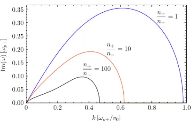
The density contrast is embedded in the dispersion relation through the density ratio,n n+ −. In the density symmetric limit,n n+ − = 1, equation (29) reduces to a biquadratic equation inω′, and we recover the analytical solution presented in (Gruzinov 2008):
Γ′ = ℑ(ω′ =) 1
(
+ k′ − − k′)
2 1 8 1 2 (30)
2 2
equation (30) gives the growth rate of the unstable modes, and is plotted in figure 3. If we develop at thefirst order in ′k the dispersion relation equation (30), we obtain
Γ′ ≃ ′k (31)
which corresponds to the KHI dispersion relation obtained in the ideal hydrodynamic model for a symmetric shearflow in the absence of surface tension and gravity (Chandrasekhar1961). The two fluids plasma model dispersion relation differs here from the classical hydrodynamics results by introducing a cut-off at ′ =k 1. There is, therefore, a maximum value of the curve that corresponds to the growth rate (Γ′max) of the fastest growing mode ( ′kmax). These quantities satisfy
Γ
∂k′ = 0 and are given by:
Γ′ = ℑ
(
ω′)
= 1 8 (32) max max and = ′ k 3 8 (33) maxThe real part of ω′ vanishes over the range of unstable modes, meaning that the unstable modes are purely growing waves, which is consistent with the symmetry of the system. Note that these electron-scale unstables modes occur when the plasma is considered to be cold, i.e.,
≪
vth v0, whereas compressible MHD or Hydro modes in an initially unmagnetized plasma are only unstable forv0 < 2cs = vth* me mi/ , which correspond to very slow (or very hot)flows (Miura and Pritchett 1982). Therefore, shear flow instabilities in initially unmagnetized conditions with fast drift velocities (relative to the temperature) can only develop on the electron-scale.
In the case of a density jump (n n+ − > 1), equation (29) has to be solved numerically. Figure3illustrates the effect of the density asymmetry on the growth rate of the unstable modes for multiple values ofn n+ −. The values of the density ratio are changed assumingn+ fixed so
that the normalizing frequency, ωp+ γ0, and wavenumber, ωp+ (v0 0γ), which determine the axes scales of figure 3, remain constant. We also consider that n+ corresponds to the denser flow.
Thus, larger density ratios are achieved by lowering the value ofn−. The qualitative evolution of the unstable modes is independent of the value ofn n+ −, indicating that the general features of the instability are maintained. When n n+ − > 1 the frequency ω′ acquires a real part over the range of unstable modes leading to propagation (figure4). The drifting character of the unstable modes results from an unbalanced interaction when each flow has different densities. The dispersion relation equation (29) in the small k limit reduces to
ω′ = ′ + − + k r r ir 1 ( ( 1) 2 ), (34) 1 4
where r = n n− +. This asymptotic result can be verified in figures 3 and 4. However, this result does not coincide with the dispersion relation obtained in the ideal hydrodynamics model when there is a density jump, Γhydro = 2k r (1 + r). As we noticed before, the two growth rates coincide only in the small k limit when r = 1. In the regime n n+ − > 1, the unstable oscillations develop differently in each flow due to their different densities. The growing oscillations are more strongly manifested in the lower densityflow (n−) and will thus drift in the direction of then− bulk flow. On the other hand, in the density-symmetric regime, the surface interaction betweenflows is balanced; the unstable modes develop equally in each flow, leading to the development of purely growing waves, as previously discussed. The typical growth rate of the ESKHI Γ
(
max ωp+)
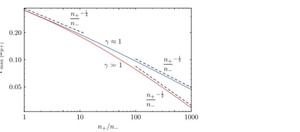
, as was observed in figure 3, slows down asn n+ − increases. This is because the shear surface current sheets decrease as n− is lowered. In the limit n− → 0 (n n+ − → ∞), we obtain a free-streaming plasma in vacuum where the development of the ESKHI is inhibited, Γmax ωp+ → 0, as expected.The scaling relations of the ESKHI withn n+ −are shown infigure5. In the similar density regime,n n+ − ≈ 1, the growth rate scales as Γmax ωp+ ∝ (n n+ −)−1 4for both relativistic and non-relativistic shears. In the high density contrast regime, n n+ − ≫ 1, the growth rate scales as Γmax ωp+ ∝ (n n+ −)−
1 3
for non-relativistic shears, and Γmax ωp+ ∝ (n n+ −)−
1/2
for highly relativistic shears. Note also that in the n+ →0 limit (ω →p+ 0), a scenario where the n−
Figure 4. Real (dashed curves) and imaginary (solid curves) parts of ω′ for the symmetric (n n+/ −=1) and an asymmetric (n n+/ −= 10) density regimes. The density symmetric and asymmetric regimes are represented by the blue and red curves, respectively.
plasma streams in vacuum, the ESKHI shuts down. At large n n+ − regimes, the ESKHI dominates over other common plasma instabilities in unmagnetized scenarios such as the Weibel and Two-Stream instabilities. The growth rates of the Weibel (Silva et al 2002) and Two-Stream instabilities (O’Neil et al 1971) scale as ΓWeibel ωp+ ∝ (n n+ −)−
1/2
and Γ2 stream− ωp+ ∝ (n n+ −)−1 3, respectively. Both growth rates decay more rapidly with n n+ − than the growth rate of the ESKHI. The physics of large density contrast settings will thus be mainly determined by the evolution of the ESKHI. Hence, in realistic astrophysical settings with high density contrasts, where various plasma instabilities are triggered simultaneously, magnetic field generation can also be attributed to the development of the ESKHI.
2.1.2. Effect of mobile ions. The influence of mobile ions on the theory previously shown is easily incorporated. The ionfluid obeys the same equations as the electron fluid and the charge and the mass of the ions are the only physical parameters that could impact the dispersion relation. For the sake of clarity, we will restrict ourselves to initial equal density plasma. Following the exact same derivation as aforesaid, we obtain a differential equation with the same form as equation (22) where the plasma frequency needs to be renormalized, ωp2 →ωp2(1+ m me i). In the case of heavy ions, mi ≫me the effect can be considered negligible. On the other hand, for an electron-positron plasma, the transverse wavenumberk⊥ (see equation (26)) is rescaled with the plasma frequency (that is multipled by 2 ) and so is the wavenumber ′kmax associated to the maximum growth rate that peaks at Γmax′ = 1/2.
2.2. Comparisons with PIC simulations
Numerical simulations were performed with OSIRIS (Fonseca et al2003, Fonseca et al2008), a fully relativistic, electromagnetic, and massively parallel PIC code. We have simulated 2D systems of shearing slabs of cold (v0 ≫ vth, where =
−
vth 10 3c is the thermal velocity) unmagnetized electron-proton plasmas with a realistic mass ratio m mp e= 1836 (mp is the proton mass), and evolve it until the electromagnetic energy saturates on the electron time scale. We explored a subrelativistic shear flow scenario with v0 = 0.2c. The setup of the numerical simulations is prepared as follows. The shearflow initial condition is set by a velocity field with
Figure 5. Scalings of the growth rate of the ESKHI (Γmax/ωp+) with the density ratio between shearing flows. The blue and red curves characterize non-relativistic (γ ≈ 1) and highly relativistic (γ ≫ 1) settings, respectively.
v0 pointing in the positive x1 direction, in the upper and lower quarters of the simulation box, and a symmetric velocity field with −v0 pointing in the negative x1 direction, in the middle portion of the box. Note that the coordinates x x( ,1 2, x3)used in the PIC simulations correspond to the cartesian coordinates( , ,y x −z) of the theory presented in the previous sections. Initially, the systems are charge and current neutral, and the shearing flows have equal densities. The simulation box dimensions are 10 × 10 (c ωp)2, where ωp =
(
ne2 ϵ0me)
1/2 is the plasma frequency, and we use 20 cells per electron skin depth(
c ωp)
in the longitudinal direction and200 cells per electron skin depth
(
c ωp)
in the transverse direction. Periodic boundary conditions are imposed in every direction and we use 36 particles per cell. In order to ensure result convergence, higher numerical resolutions and more particles per cell were tested.2.2.1. Equal density shear flows. We begin by analyzing a subrelativistic shear scenario (v0 = 0.2c) where the counter-streaming flows have equal densities. The evolution of the electron density of the system is depicted infigure 6, where the signature roll-up dynamics at the end of the linear phase of the ESKHI is observed. The protons of the system remain unperturbed (free-streaming) at these time scales due to their inertia. The wavelength of the growing perturbations in the electron density measure 2c ωp, which corresponds to the wavelength of the fastest-growing mode given by equation (33). The magnetic field structure excited by the instability is shown infigure7. Thefirst inset of figure7is taken during the linear phase of the ESKHI, showing the surface wave structure of the magnetic field, which is consistent with the two-fluid theory. The wavenumber parallel to the flow matches that of the theoretical fastest growing mode (equation33), and the wavenumber perpendicular to theflow is evanescent. During the linear phase, the amplitude of the magneticfield grows exponentially (seefigure8(a)) with a growth rate of0.33ωp, in close agreement with the theoretical prediction of equation (32) Γ
(
= 0.35ωp)
. As the instability develops, the growing perturbations become strong enough to distort the sharp boundary between the shearingflows, allowing them to mix. This mixing can no longer be treated with a fluid description, since the system dynamics becomes intrinsically kinetic. The signature of this kinetic regime is observed in figure 7(b1), where a DC component(
k1= 0 mode)
of the magnetic field begins to develop on top of theFigure 6.Electron density structures at (a) ω =pt 35, (b) ω =pt 45, and (c) ω =pt 55. The two flows stream with velocitiesv0= ± 0.2cex1
Figure 7.(1) B3 component of the magnetic field in the xy plane and (2) corresponding average of the Fourier transform in k1at times (a) ω =pt 35, (b) ω =pt 45, and (c) ω =pt 55.
Figure 8. Temporal evolution of the energy equipartition ϵ ϵB/ p in scenarios (a) shear between equal density flows, and (b) shear between flows with density contrast
= + −
harmonic structure previously generated during thefluid regime. This DC magnetic field is not unstable according to thefluid model, as can be seen in equation (30). The evolution of the DC magnetic field mode is clearly illustrated in figure 7(a2–c2), which shows the Fast Fourier Transform (FFT) spectrum in k1 of the magnetic field in the system. At early times, the FFT spectrum reveals a peak aroundk1= 3ωp c, which corresponds to the unstable mode of thefluid regime (figure 7(a2)). At later times, however, the growingfields developed in the linear stage of the instability lead to electron mixing/interpenetration between the twoflows, resulting in the development of the DC mode (figure7(b2)). Furthermore, when the instability saturates, the DC mode is the dominant component of the magneticfield, as shown in figure7(c2). The physical picture underlying the growth and evolution of the DC mode of the magnetic field will be discussed later in section 3.
2.2.2. Different density shear flows. The density contrast effects predicted by the theoretical two-fluid model have also been verified with numerical simulations. Figure 9 shows the development of the electron density structures for a density contrast setting withn n+ − = 10. The ESKHI modulations that eventually turn into vortices are strongly manifested in the lower-density plasma cloud (represented by the blue flow in figure 9). The typical length of these modulations is larger than those of the density symmetric case, as predicted by the theoretical model, measuring λ≃ 3.3c ωp+. This value agrees with the theoretical wavelength of the
fastest-growing mode, λmax = 3.1c ωp+. The self-generated magnetic field structure is represented in figure 10, where the asymmetry in the evanescent behaviour of the surface mode in the different density regions can be observed. The growth rate of the instability is lowered with respect to the equal-density case and is in good agreement with the linear theory (figure 8(b)).
2.3. Finite velocity shear gradient
The analytical treatment of the effect of afinite velocity shear gradient (smooth velocity shear profile) on the development of the electron-scale KHI is not trivial. The details of the underlying mathematics and numerics can be found in the appendix.
Figure 9.Electron density structures for a shear flow with n n+/ −=10 at (a) ω =pt 60,
wavenumber corresponding to the maximum growth rate follows a similar trend by slightly decreasing when the parameter k L increases. For arbitrarily large⊥ k L, an exact numerical⊥ solution for the dispersion relation of the electron-scale KHI can be found, and we discuss a numerical scheme in the appendix.
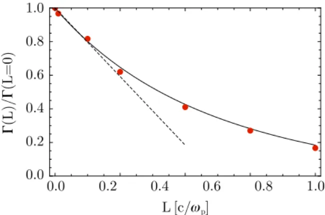
The above analytical and numerical results have been verified with PIC simulations. The setup of the simulations is identical to those previously described, only replacing the discontinuous velocity profile with the smooth function v x0( ) = V0 tanh ( / )x L . This profile is also used in the numerical algorithm to solve the dispersion relation in thefinite gradient shear scenario. The measurement of the maximum growth rate in the simulation is done by following in time the peak of the Fourier spectrum of one of thefield structures during the linear phase of the instability. Figure 11 displays the maximum growth rate as a function of the gradient length for equation (81), the numerical solution and the simulations results (V0 = 0.2c). For small values of the parameter k L, i.e.,⊥ L ≪0.3c ωp (k⊥ ∼ 3ωp c forV0 = 0.2c), equation (81) is in good agreement. For higher values of the gradient length, equation (81) is not valid since it was derived in the first order of k L. Nevertheless, the numerical solutions show a⊥ very good agreement with the simulation results, where we observe a decay of the maximum growth rate. Both the equation (81) and the numerical solution have been verified with PIC simulations for various values of V0 and are both in good agreement. We have observed the development of the electron-scale KHI with PIC simulations for L up to10c ωp (Grismayer
et al2013).
3. DC magnetic field generation in unmagnetized shear flows
For the sake of completeness, we review in this section the main results of the DC magnetic field generation mechanism in unmagnetised shear flows which are outlined in (Grismayer et al 2013). We then present a more detailed analysis of the equipartition fields and the dependence of the equipartition number on the dimensionality of the model.
In the previous section, numerical simulations showed the growth of a DC (k = 0) magnetic field mode (figure 7(c) and figure 10(c)), which is not predicted by the linear fluid theory (figure 3), Γ′ ′ =(k 0)) nor has it been previously identified in MHD simulations. Only kinetic simulations (Alves et al2012, Boettcher et al 2012, Grismayer et al 2013) have been able to capture this mode. The growth of the DC magneticfield mode results from a current imbalance due to electron mixing across the shear interface, while the ionflows remain almost unperturbed due to their inertia. The orientation of the DC magneticfield peak is determined by the proton current structure. The mixing arises due to the deformation of the electron interface between the two flows which, in the linearized fluid calculations, is not accounted for and, in the zeroth
Figure 10.(1) B3component of the magneticfield withn n+/ −= 10 in the xy plane and (2) corresponding average of the Fourier transform in k1 at times (a)) ω =pt 60, (b))
ωpt=75, and (c)) ω =pt 90.
Figure 11.Evolution of the maximum growth rate as a function of the gradient length. Dashed curve: expression (81); plain curve: numerical algorithm; red dots: PIC simulations for v x c0( )/ = 0.2tanh x L( / ).
order, remainsfixed. Alternatively, we find that the physics describing the formation of a DC mode can be modeled in a 1D reduced theory where an initial temperature drives the mixing effect.
3.1. Warm shear flow
We discuss here the temperature effect in a shearflow scenario, and its role in the generation of a DC magneticfield mode along the shear. For the sake of simplicity, and without loss of generality, we assume a simple sharp velocity shear transition between two plasmas with equal temperatures. We consider that the temperature is sufficiently high such that the electron thermal expansion time scale is much faster than the electron expansion induced by the onset of the fluid KHI in an equivalent cold scenario. The theoretical setting of the system is illustrated in figure 12(a). We consider only the electron thermal velocity, neglecting the thermal velocity of the protons due to their inertia. Since we are interested in describing the DC phenomena, all derivatives along the x direction vanish, reducing the system to the 1D problem displayed infigure12(b). We, therefore, consider the purely one-dimensional case where the particles can move along x, as infigure12(b). Initially all the fields are zero and we assume a warm initial plasma with a tangential shear flow identical to the one described in section 2.1 with an initial temperature such as vth ≪ v0. This setting is not in Vlasov equilibrium and it is clear that the thermal expansion of the electrons across the shear surface (ions are assumed to be cold and free streaming) leads to an imbalance of the current neutrality around the shear surface, forming a DC magnetic field in z direction. The initial corresponding electron distribution function reads
= = −
f x v v v t( , x, y, z, 0) f v v0( ,x y v0sign( ),x vz) (36) The situation can be seen as two thermal plasmas with shearing counter-propagating fluid velocities. The thermal expansion of the electrons (the ions, due to their inertia, are assumed to be free streaming) across the shear will transport an electron current on the order ofen v0 0, with a characteristic width ofv tthx . This should lead, at early times, to the formation of afield Bz around the shear of widthv tthx and magnitude of μ en v v tthx
0 0 0 . This is the underlying physical picture of
the DC magneticfield growth. Due to the dimensionality of the problem, it is clear that E Bz, x,
and By remain zero. The reduced set of equations is
−∂ ∂ = ∂ ∂ B t E x (37) z y μ −∂ ∂ = + ∂ ∂ B x J E t c 1 (38) z y y 0 2 μ = −∂ ∂ J E t c 1 (39) x x 0 2 ∂ ∂ + ∂ ∂ − + × ∂ ∂ = F t v F x e m F E v B v ( ). 0 (40) x z where
∫
= F x v v t( , x, y, ) dvf x v v v tz ( , x, y, z, ) (41)The formal solution of the Vlasov equation equation (40) is =
F x v v t( , x, y, ) F x0( ,0 vx0, vy0) (42)
where x0, vx0 and vy0 denote the position and velocities of an electron at t = 0 and f0 =
∫
dv Fz0 0.At early times, if we assume that the inducedfields are sufficiently small that we can neglect the change of momentum of the electrons, the distribution can be solved along the free-streaming orbits, i.e., x = x0 + v t vx0 , x= vx0, vy = vy0. For the sake of simplicity, we divide the initial
electron distribution into two parts, F0 = F0−(x0 < 0)+ F0+(x0 > 0), corresponding to the two initially separated flows. In the approximation of free-streaming orbits, the electron currents read
∫
∫
≃ − − ∓ ± ± Je y, e dv vy y dv fx 0 (x v t v vx, x, y v0). (43) With f0±( ,x0 vx0, vy0 ∓ v0) = n f0M(vx0)fM(vy0 ∓ v0), where = π − fM( )v e v v 2 vth 2th 2 2 represents the Maxwellian velocity distribution, we obtain for the electron currents∫
≃ ∓ ± ∓ ∞ Je y en v dv f ( )v (44) x t x M x , 0 0 ≃∓ ⎛ ∓ ⎝ ⎜ ⎞ ⎠ ⎟ ev n x v t 2 erfc 2 thx (45) 0 0The total current is obtained by adding the unperturbed proton currents. This yields
= − + ⩽ ⎡ ⎣ ⎢ ⎢ ⎛ ⎝ ⎜ ⎞ ⎠ ⎟⎤ ⎦ ⎥ ⎥ J ev n x v t x 2 erfc 2 0 (46) y thx 0 0 = ⎛ > ⎝ ⎜ ⎞ ⎠ ⎟ J ev n x v t x erfc 2 0. (47) y thx 0 0
The magneticfield is then simply given by the Maxwell-Ampere equation, equation (38), where the displacement current is neglected
magnetic energy growing in the system is given by
∫
ϵ μ μ = dx B ≃ en v v t 2 0.156 2 ( ) ( ) , (50) B z thx 2 0 0 0 0 2 3 with∫
du u[| |erfc ( )| | −u e−u2 π]2 ≃ 0.156.As was pointed out, this derivation is only valid as long as the orbits of the electrons do not diverge much from the free-streaming orbits, i.e., as long as the electric and magneticfields that develop in the expansion process do not affect the free motion of the particles. In fact, there are two phenomena that affect the growth of the magneticfield. First, the electrons will eventually feel the induced magnetic field which tends to push more electrons across the shear via the
×
v0 Bz force. This will increase the rate of current transported and, thus, will increase the
growth rate of the magneticfield. One should note that, at first, only the magnetic field acts on the electrons since the electric field Ex remains zero in our model: the initial temperature is uniform in space and, therefore, there are as many electrons crossing from the left as from the right. The charge neutrality is then conserved in the system. A crude estimate of the time at which our model breaks can be made considering that only the slow electrons, initially around the shear, will experience a strong velocity change due to the peaked shape of the magnetic field. Therefore, the model will break down approximatively when an electron initially at rest (around x = 0) acquires a velocity change on the order of vthx, which corresponds to a strong distortion of the Maxwellian distribution function around the shear. This can be written for the velocity change as
∫
δ ω π ∼ ′ ′ ∼ ⎜⎛ ⎟ ⎝ ⎞⎠( )
v ev m dt B t v v c t (0, ) 2 . (51) x t z thx p 0 0 0 2 2It follows that the model is valid until ωpt ∼ (2 )π c v
1 4
0. Second, the growth of the magnetic
field induces an electric field Eythrough the Maxwell–Faraday equation (equation (37)). We can
estimate, through the characteristic time t and length of the problemv tthx , the magnitude of the field, Ey ∼ v Bthx z. Inserting the value of Ey into the Maxwell–Ampere equation, we find the
displacement current term ∂Ey ∂t leads to a v(thx c)
2
correction to the DC magneticfield peak at early times. However, the displacement current tends to increase the electron current on either side of the shear interface, eventually building the DC magnetic field side wings observed at later times (figure 13(a3)–(b3)).
In order to verify our analytical calculations and to further investigate the phase at which the electrons deviate from their free-streaming orbits, we have simulated a shearflow between
Figure 13. Evolution of the electron phasespace (insets a1–3 and b1–3) and DC magnetic field peak (insets a4 and b4); log–log is used to display linear DC peak evolution in inset a4, and log–linear is used to display exponential evolution in inset b4. Left: 1D warm shearflow with =v0 0.2candvth= 0.016c. Right: 2D cold shearflow for
the same v0. The blue (red) color represents the electrons with a negative (positive) drift velocity v0. The self-consistent DC magnetic field is represented by the solid curve, whereas the dashed curve represents the magnetic field given by the theoretical model.
distribution function in the shear region is shown at ωpet = 17. The model underestimates the magnitude of the magnetic field and one can clearly observe the distortion of the distribution function in thefield region. As the magnetic field grows, the Larmor radius (rL) of the electrons crossing the shear interface decreases. When the minimum rL,min (associated to the peak of BDC) becomes smaller than the characteristic width of the magneticfieldlDC, the bulk of the electrons becomes trapped by the magneticfield structure. This is illustrated in figure13(a3) at ωpet = 55. The magnetic trapping prevents the electron bulk expansion across the shear (which drives the growth of the magneticfield), saturating the magnetic field. An estimate of the saturation can be obtained by equatingrL,min ∼ lDC. From equation (49), it is possible to write the magneticfield as BDC( , )x t = 4πen0 0βw x t( , ), where w(0, ) should be interpreted as the characteristic widtht of thefield. With lDC ∼ w(0, )t ,rL,min= mv0 0γ eBDC(0, )t , we find thatlDC ∼ c γ ω0 pe, giving
the saturation level of the magnetic field as
ω ∼ β γ eB m ce pe . (52) DC sat 0 0
This scaling has been verified for 1D simulations (see figure 3 in (Grismayer et al 2013)) for which the bestfit function matching the simulation is eBDCsat m ce ωpe = 1.9β0 γ0.
3.2. Cold shear flow
In the absence of an initial temperature, an alternative mechanism is needed to drive the electron mixing across the shear surface that, in turn, generates the DCfield. This mechanism is the cold fluid ESKHI that has been thoroughly discussed in section 2. In fact, in the warm shear flow scenario, both the cold fluid ESKHI and the electron thermal expansion can contribute to the generation of the DC field. This occurs when the typical length of the DC field, due to the thermal expansion (lDC) after a few e-foldings of the cold fluid ESKHI (TKHI growth− = Ne foldings− Γmax, where Ne foldings− is on the order of 10), is on the order of the relativistic electron skin depth, i.e., v Tth KHI growth− ∼ γ0c ωpe. Therefore, the cold fluid ESKHI dominates the electron mixing in the limit
γ ω ≪ − v Tth c . (53) pe ESKHI growth 0
For a two-dimensional cold plasma undergoing the ESKHI, the electron distribution function can be written as
δ δ δ
= − −
(
)
(
) (
)
f x y v v v t, , x, y, z, n0 vx vxfl( , , )x y t vy vyfl( , , )x y t ( )vz (54) where vxfl, vyflcorresponds to the velocityfield solutions of the fluid theory. In this case, the
self-generated ESKHI fields play the role of an effective temperature that transports the electrons across the shear surface, while the protons remain unperturbed, inducing a DC component in the current density, and hence in thefields. We then have to solve the evolution of the distribution function and show that the current densityJy, averaged over a wavelength λ = 2π k∥, has a non-zero DC part. We follow the same approach as before and calculate the average distribution function, defined as:
∫
∫
∫
λ =
λ
(
)
F x v t( , x, ) 1 dvy dvz dyf x y v v v t, , x, y, z, . (55)
To obtain analytical results we will assume that the linearly perturbedfluid quantities are purely monochromatic, which is equivalent to assuming that after a few e-foldings, the mode corresponding tok∥= k∥maxdominates with a growth rate of Γ = Γmax. We then writevyfl ≃ v x0( ) andv = ¯v sin (k y e∥ ) − | |+⊥ Γ
xfl xfl
k x t
, wherev¯xfl, the amplitude of the velocity perturbations at t = 0, is associated with the small thermal fluctuations (small enough to ensure that the thermal expansion is negligible overTESKHI growth− ). Inserting vxfl, vyfl into equation (55), we obtain
π ξ = − F x v t n v ( , , ) 1 , (56) x max 0 2
where ξ( ,x v tx, )= v vx max( , )x t with = ¯
Γ
− | |+⊥
vmax( , )x t v exfl k x t
. We observe that the development of 2D cold ESKHI reveals close similarities with the 1D hot model previously described. In the 2D ESKHI, averaging the distribution in the direction of the flow shows that the perturbation gives rise to a spread invx that may be interpreted as an effective temperature. The spread invx
decays exponentially away from the shear and grows exponentially with time. The mean velocity is zero and the effective temperature associated with this distribution function is defined as
∫
= = V x t n dv v F x v t v ( , ) 1 ( , , ) 2 . (57) eff x x x max 2 0 2 2One can then expect a similar physical picture to that of the hot shear scenario and, as a result, the emergence of DC components in the fields which are induced by the development of the unstable ESKHI perturbations. The evolution of the phase space in figure 13 illustrates the similarity between the warm 1D (insets a1–3) and cold 2D (insets b1–3) scenarios.
The challenge in this scenario is to determine how such a distribution function expands across the shear surface due to the complexity of the orbits in the fields’ structures (multidimensional fields with discontinuities at x = 0). One can, however, overcome this difficulty by solving the expansion along approximate orbits. This procedure, although not self-consistent, gives rich qualitative and quantitative insight regarding the features of the current that develop around the shear interface. In thexpx phase space, the electrons describe outward-spiraling growing orbits, since they are drifting across the standing growing perturbation. In the region where the electron mixing occurs, we assume electron orbits given by
Γ ∼ +
(
)
Γ x x vx e t 0 0 and ∼ Γvx v ex0 t where x0 and vx0 are the position and velocity of a particle
particle that was originally in the vicinity of the shear. The limits of the integral in equation (59) represent the deformation of the boundary between the twoflows on a characteristic distance of
Γ
vmax0 as the instability develops. In the fluid theory, the boundary remains fixed, precluding the development of the DC mode. We thenfind the total current density by summing the proton contribution and integrating to obtain the induced DC magnetic field:
β ζ π ζ ± ⩾ = ∓ ⎡ ∓ ± − ⎣ ⎢ ⎤ ⎦ ⎥ B ( x 0, )t 8en x arcsin( ) 2 1 1 (61) DC 0 0 2
with ζ= Γx vmax0 . The peak of the DC magnetic field is located at x = 0 where the expression above reduces toBDC(0, )t = 8e n vβ0 0 max0 ( ) (t πΓ)and thus grows at the same rate as the ESKHI fields. One can verify in figure13(b1–b2) that equation (61) shows reasonable agreement with the 2D simulations. This derivation neglects the DC Lorentz force on the electron trajectories, which makes this model valid as long as the induced DCfields remains small compared to the fluid fields associated to the modek∥max. The peak of the BDCfield is proportional to vmax( )t
0
that represents the maximum value of the fluid velocity vxfl,which obeys
β γ ω
= −
(
+)
(
− ∥)
vxfl ie Exfl 0Bzfl me0 k v0 . From the linear fluid theory,one can compute the ratio
Bzfl Exfl from which we deduce that for sub-relativistic shears (γ ∼ 10 ), ω
∼
vxfl ec 2 7 Bzfl me pev0 implying BDC ∼ (8 7 )π Bzfl and that for ultra-relativistic shears
(γ ≫ 10 ), vxfl ∼ e Bzfl m ce 2ω γpe 03 2 yielding BDC ∼ (4 π)Bzfl. We conclude that the induced DC magnetic field is always on the same order as the fluid fields and thus its consequences to ESKHI development cannot be neglected. As the DCfield evolves, electrons start to get trapped and we expect a level of saturation similar to the saturating level obtained in the 1D model. This has been verified by the simulations. The comparisons between the saturation level of the 1D, 2D, and 3D simulations are shown in figure 3 in (Grismayer et al 2013), also verifying the β0 γ0 scaling. One can also compute the equipartition number related to the magnetic field at saturation. Using equation (52) one finds
∫
∫
ϵ π γ γ γ = + − ∼ +(
)
dxB dxn m m c m m 8 ( 1) 1 2 1 (62) l l e p e p DC sat 2 0 2 0 0 0 DC DCwhich is similar to the equipartition number found for the Weibel instability (Medvedev and Loeb1999). Our derivation for the saturation of the DC magneticfield also allows recovery of the empirical estimate of (Alves et al 2012) already given for such a shear scenario. When a
smooth shear is considered, the electron KH still develops as we have shown in section2. We verified that the initial electron transport across the shear, due the development of the instability, is the mechanism triggering the magnetic field generation, therefore validating the physics captured by our model. At saturation the DC magneticfield has a typical width on the order of the initial shear gradient length. Keeping the same arguments that we have used to derive the approximate value of the DC field at saturation, i.e.,rL,min ∼ L implies
ω ∼ ˜ = ˜ eB m c B L L ( 0) (63) e pe DC sat DC sat with L˜ = Lωpe c γ
0. Such a scaling has been verified for ωL pe c ≫ 1 and the comparison
between the crude estimate and the simulations is presented infigure 14. Interestingly, the DC magneticfield remains stable beyond the electron time scale and persists up to 100 s ωpi−1 (see figure 1 in (Grismayer et al 2013)), which is the regime of validity of the equation (63). Eventually the protons will drift away from the shear surface due to the magnetic pressure, broadening the DC magnetic field structure and lowering its magnitude. On much longer time scales, the corresponding proton dyanamics, associated with the DC magnetic field pressure, will lead to the formation of a double-layered structure (Liang et al 2013). This long time evolution of the DC magnetic field will be explored elsewhere.
4. Particle acceleration
We investigate in this section the acceleration of particles due to the development of electron-scale shear instabilities. Particle acceleration in shearflows has been previously investigated by many authors, mainly related to astrophysical scenarios (Berezhko and Krymskii1981, Jopikii and Morfill 1990, Ostrowski 1990, Rieger and Duffy 2005, Rieger and Mannheim 2002, Webb1989). The shear acceleration mechanism (Rieger and Duffy2005) is based on the idea that energetic particles may gain energy by systematically scattering off moving small-scale magneticfield irregularities. These irregularities are thought to be embedded in a collisionless
Figure 14.Magnitude of the DC magnetic field peak at saturation as a function of the initial shear gradient length for v c0/ =0.2. The error bars are associated with the fluctuations of the peak value in the saturation stage. The dashed line represents the best fit curve to the simulation results, given by eBDCsat/m ce ωpe = 0.2/(1+ 0.6Lωpe/ )c .
shear flow such that their velocities correspond to the local flow velocity. In the presence of velocity shear, the momentum of a particle travelling across the shear changes and the acceleration process essentially draws on the kinetic energy of the backgroundflow. In the shear flows we discussed in the previous sections, fluid and kinetic effects lead to the emergence of organized electric and magnetic fields that are maintained in the shear region up to ion time scales. The electronsflowing in the shear region experience strong acceleration in these fields and also emit strong radiation while gyrating in the DC magnetic field. This acceleration process therefore differs from the shear acceleration mechanism of (Rieger and Duffy 2005).
In order to investigate the acceleration of electrons in the shear due to the self-generated fields, we performed a 2D simulation of a relativistic cold shear flow, γ = 30 , v cth = 10−
3
. The simulation domain dimensions are250×2000 (c ωp)
2
, resolved with 10 cells per electron skin depth Δ
(
x1 = Δx2 = 0.1c ωp)
and 36 particles per cell per species are used. The shear flow initial condition is set by a velocity with +p e→0 1 forx2 > 0and a symmetricflow with − →p e0 1 for
<
x2 0. We impose periodic and absorbing boundary conditions in the x1 and x2 directions, respectively. The transverse direction x2 has been extended up to 2000c ωp with an absorbing boundary condition in order to avoid particle recirculation over the shear region, which tends to produce unphysical additional acceleration. The dimension of the simulation box allows us then to follow the evolution of the system until ω ∼pt 1000, the time at which some particles approach the boundaries of the box. This is critical to guarantee that the spectrum of accelerated particles reproduces the physics associated with acceleration in a single shear transition region. The growth rate and fast-growing mode in the early development of the relativistic electron-scale KHI was found to agree with the theoretical predictions of section 2. As explained in section 3, the nonlinear development of the instability drives the mixing between electron populations at the shear interface and generates DC components in thefields. At full saturation of the instability, the persistent electric and magnetic field components are on the order of γ0meωpc e. During the early stage of the instability the oscillating fields are responsible for acceleration and deceleration of the electrons. This results in a slight temperature increase of the plasma and the electron distribution function widens around the mean energy γ0. Once the
instability saturates, the electrons can experience strong acceleration due to the long-lived electric field structures in the shear region. Furthermore, the DC magnetic field, which remains intense only in the shear region, provides one of the mechanisms to curve the electron trajectories and hence takes part in the thermalization and isotropization of the electron distribution function.
The energy distribution function of the electrons is plotted in figure 15 at ω =pt 0 and ωpt = 1000. The final distribution can be separated into three distinct parts. The low energy part,1 < γ < 5, corresponds to a thermal Juttner distribution, f( )γ ∼ γ2e−μγ with μ ∼ 1 γ0. The medium energy part exhibits a power law γ−5 up to γ ∼ 25. Finally, after the elbow of the distribution, one notices a hot tail that extends up to γ = 80.
To gain deeper insight into the acceleration process of the most energetic electrons in the shear region, we followed various electron trajectories whosefinal energy lay in the second and third part of the distribution shown infigure 15. Figure16 shows segments (on every inset the electron is tracked during ω ∼pt 100) of two electron trajectories. The two electrons are initially
Figure 16.Trajectories of two electrons during the non-linear phase of the instability. The varying color displayed along the trajectories stands for the energy of the electrons during the acceleration process. The black and white background represents the total electric field magnitude.
in the vicinity of the shear, as shown infigure16(a). The black and white background represents the total electric field magnitude. The growing middle structure represents the DC part of the field, whereas the modulated patches on both sides originate from the saturated unstable modes. One can clearly see that most of the acceleration occurs when the electrons cross the electric field patches. The magnitude of the electric field patches is mainly due to the transverse component E2, whereas the acceleration takes places in the x1direction. After being accelerated, the particle can cross the shear to be finally reaccelerated on the patches of the other side or definitively leave the shear region. The time evolution of the energy of the two tracked electrons is shown in figure 17. As explained previously, the energy of the electrons does not increase significantly until ω ∼pt 300which corresponds to the saturation of the ESKHI. Soon thereafter, both electrons experience a strong energy kick, Δγ ∼ 30 at around ω ∼pt 50. At ω ≃pt 430, the
electrons have acquired their maximum energy which then remains constant, indicating that they have left thefield-dominated shear region. The electron denoted by e1crosses the shear without really being affected by the transverse component of the electric field, while the electron e2 experiences a strong deceleration before eventually leaving the shear region.
One can understand the acceleration mechanism if one sees the process as relativistic electrons surfing on the electric field patches, flowing with the plasma, which can be assumed to be constant in magnitude. First it is necessary to quantify the magnitude of the three electromagnetic components. Using equations (15), (17), and (20), we obtain the following ratio in the limit γ ≫ 10 : E E1 2 ∼ 1 2γ0 and E B2 3 ∼ 1. If we assume that this ratio still holds during the non-linear phase, then the orbits of the electrons, approximatively streaming in the x1direction with the Lorentz factor of γ0, are mainly governed by Ex2 and Bx3. The equations of motion read
= − = − ⎜⎛ − ⎟ ⎝ ⎞⎠ dp dt e cv B dp dt e E v cB , . (64) 1 2 3 2 2 1 3
In the case E2= B3, the solution for the trajectory of the electron is given by (Landau and Lifshitz1975) α ϵ α = − + + p c c p c 2 2 (65) 1 2 2 2 2