Introducing additional factors for the Brazilian market in the fama-french five-factor asset pricing model

Texto

(1)FUNDAÇÃO GETULIO VARGAS ESCOLA DE ECONOMIA DE SÃO PAULO. LEONARDO MATHIAZZI LAGNADO. INTRODUCING ADDITIONAL FACTORS FOR THE BRAZILIAN MARKET IN THE FAMA-FRENCH FIVE-FACTOR ASSET PRICING MODEL. SÃO PAULO 2016.

(2) LEONARDO MATHIAZZI LAGNADO. INTRODUCING ADDITIONAL FACTORS FOR THE BRAZILIAN MARKET IN THE FAMA-FRENCH FIVE-FACTOR ASSET PRICING MODEL. Tese apresentada para a Escola de Economia de São Paulo da Fundação Getulio Vargas, como parte dos requisitos para a obtenção do grau de Mestre de Economia. Campo de conhecimento: Finanças. Orientador: Prof. Dr. Ricardo Ratner Rochman. SÃO PAULO 2016.

(3) Lagnado, Leonardo Mathiazzi. Introducing Additional Factors for the Brazilian Market in the Fama-French FiveFactor Asset Pricing Model / Leonardo Mathiazzi Lagnado. - 2016. 64 f. f. 65 Orientador: Ricardo Ratner Rochman Dissertação (MPFE) - Escola de Economia de São Paulo. 1. Ações (Finanças) - Brasil. 2. Mercado de capitais - Brasil. 3. Avaliação de ativos - Modelo (CAPM). 4. Avaliação de riscos. I. Rochman, Ricardo Ratner. II. Dissertação (MPFE) - Escola de Economia de São Paulo. III. Título.. CDU 336.767(81).

(4) LEONARDO MATHIAZZI LAGNADO. INTRODUCING ADDITIONAL FACTORS FOR THE BRAZILIAN MARKET IN THE FAMA-FRENCH FIVE-FACTOR ASSET PRICING MODEL. Tese apresentada para a Escola de Economia de São Paulo da Fundação Getulio Vargas, como parte dos requisitos para a obtenção do grau de Mestre de Economia. Campo de conhecimento: Finanças. Aprovação: 23 de agosto, 2016. Membros da banca: ___________________________ Prof. Ricardo Ratner Rochman FGV-EESP. ___________________________ Prof. Claudia Emiko Yoshinaga FGV-EESP. ___________________________ Prof. Joelson Oliveira Sampaio FGV-EESP.

(5) Dedication I gratefully dedicate this thesis to my wife, Celina, who was always understanding, loving and supportive, as well as to my parents, who placed so much value in education and made it possible for me to come this far.. 5.

(6) Acknowledgements The completion of this thesis could never had been possible without the assistance of so many people who participated in my education thus far. I truly appreciate their contributions. Nevertheless, I would like to give special thanks to Professor Ricardo Ratner Rochman for his uninterrupted support, as well as to all the committee members. I also thank my wife, Celina, for proofreading my document so many times and Fernando Kamitani for his help with naming specific terms and variables.. 6.

(7) Abstract This dissertation is aimed at evaluating the risk-return relationship of stocks by incrementing the Fama and French five-factor model (F. FAMA and R. FRENCH, 2015) with two new variables. This was done by creating a six-factor model aimed at capturing the size, value, profitability, investment and governance patterns in average stock returns. An additional seven-factor model was also created by adding a herding factor. Governance and herding were chosen as additional factors because of a hypothesis that they would be relevant in less efficient markets such as Brazil. The evaluation of the two model´s performance versus the traditional five-factor model was performed next, as well as the assessment of relevance of the newly added factors. Testing the six-factor model, it had a similar performance to the fivefactor model, and the governance factor proved to be relevant in the Brazilian market. Adding the herding factor weakened the results, although the factor still proved to be relevant in some cases.. Keywords: three-factor, five-factor, seven-factor, size, value, book-to-market, profitability, investment, governance, herding, SMD, HML, RMW, CMA, SMF, CSSD, CAPM, Capital Asset Pricing Model, stock returns, risk-return relationship. 7.

(8) Resumo O objetivo desta dissertação é avaliar a relação risco-retorno de ações incrementando o modelo de cinco fatores de Fama e French (F. FAMA and R. FRENCH, 2015) com duas novas variáveis. Isso foi feito criando um modelo de seis fatores que busca capturar os padrões de tamanho, valor, lucratividade, investimento e governança nos retornos médios de ações. Um modelo adicional de sete fatores também foi criado adicionando um fator para o efeito manada. A governança e o efeito manada foram escolhidos como fatores adicionais por conta da hipótese de que eles seriam relevantes em mercados menos eficientes como o Brasil. A avaliação da performance dos dois modelos contra o modelo tradicional de cinco fatores foi então realizada, bem como a avaliação da relevância dos novos fatores. Testando o modelo de seis fatores, descobrimos que ele tem uma performance semelhante ao de cinco fatores, e o fator de governança mostrou ser relevante no mercado Brasileiro. Adicionando o fator para o efeito manada enfraqueceu os resultados, embora o fator ainda se mostrou relevante em alguns casos.. Palavras-chave: três fatores, cinco fatores, sete fatores, tamanho, valor, book-to-market, lucratividade, investimento, governança, efeito manada, SMD, HML, RMW, CMA, SMF, CSSD, CAPM, Capital Asset Pricing Model, retornos de ações, relação risco-retorno. 8.

(9) List of Tables and Graphs Table 1: Summary of factors in the five-factor model........................................................... 17 Table 2: Carvalhal da Silva and Leal’s Corporate Governance Index (CGI) Questions ......... 24 Table 3: Governance Questions for the Seven-Factor Model ................................................ 27 Table 4: Summary of factors and portfolios in the seven-factor model ................................. 29 Table 5: Portfolio Summary Statistics .................................................................................. 32 Table 6: Sub-factor Summary Statistics................................................................................ 34 Table 7: Factor Summary Statistics ...................................................................................... 35 Table 8: Correlation of factors ............................................................................................. 35 Graph 9: Factor Relevance Summary ................................................................................... 36 Table 10: Factor Relevance Analysis ................................................................................... 37 Table 11: Consolidated Alpha Analysis................................................................................ 38 Table 12: GRS Statistics ...................................................................................................... 39 Table 13: Consolidated Alpha Analysis without HML ......................................................... 40. 9.

(10) Table of Contents 1. Introduction .................................................................................................................. 11. 2. Literature Review ......................................................................................................... 12. 3. The Seven Factor Model ............................................................................................... 25. 4. Model Results............................................................................................................... 32. 5. Conclusions .................................................................................................................. 40. 6. References .................................................................................................................... 44. 7. Appendix A – Corporate Governance Index.................................................................. 48. 8. Appendix B – Detailed Outputs of Regressions............................................................. 49. 9. Appendix C – Number of Shares in each Portfolio ........................................................ 61. 10. Appendix D – Time Series for the Seven Factors....................................................... 62. 11. Index ......................................................................................................................... 65. 10.

(11) 1 Introduction The discussion regarding the Capital Asset Pricing Model (CAPM) has been two-pronged. On one side, there is empirical evidence to support the model (SCHOLES, BLACK and JENSEN, 1972) (FAMA and MACBETH, 1973). Nevertheless, posterior developments pointed to the existence of anomaly variables in empirical tests, leading to the conclusion that beta as a singular explanatory variable for asset returns is not complete (F. FAMA and R. FRENCH, 2008). Other variables have been included and tested empirically to improve the model, such as book-to-market (B/M), operating profitability, market capitalization (size) and investment in capital expenditures (investment), all of which showed a relationship with expected returns. These variables have added explicative value to the performed regressions (F. FAMA and R. FRENCH, 1992) (NOVY-MARX, 2013) (BANZ, 1981) (TITMAN, WEI and XIE, 2004) (CARNEIRO MARTINS and EID JR., 2015). Recent testing methodologies have focused on multi-factor models. One of the most used methodologies is the empirically motivated Fama-French three-factor model. Their model introduces three systematic factors, which are firm size, book-to-market ratio (B/M) and the market index. The model became famous for its ability of showing the risk-return relationship better than the established CAPM (F. FAMA and R. FRENCH, 1993). Later, inspired by authors who showed the relevance of additional variables, Fama and French proposed a new model with five factors, now including investment and profitability. They found that the fivefactor model is superior to the three-factor model to explain the cross-section of average returns (F. FAMA and R. FRENCH, 2015). In the spirit of other models that have been developed by authors, the objective of this paper is to move on to other factors that could better explain the risk-return relationship. The rationale as to why this project is an important addition to the current body of knowledge is that there are still gaps in current models, since alpha has not yet been completely reduced to zero (F. FAMA and R. FRENCH, 1992) (NOVY-MARX, 2013) (BANZ, 1981) (TITMAN, WEI and XIE, 2004) (CARNEIRO MARTINS and EID JR., 2015). New factors could improve this and further reduce alpha. We investigate if the five original Fama & French factors can be complemented by two other factors that could prove to have some significance in the case of the Brazilian market, more 11.

(12) specifically. The reason for focusing on an emerging market is related to questions about its efficiency. This apparent lack of efficiency in Brazil suggests that adding a factor for herding behavior could be effective. Moreover, the Brazilian market has a category of companies that seem to strive for better governance factors, and market participants tend to say these stocks have a better performance. Governance, therefore, could also be an included factor. With this, we propose a new seven-factor model in this paper. The hypothesis is that both new factors will prove statistically significant and will lower the significance of the alpha of the model closer to zero. The main findings of this paper were that both the governance and the herding factors are relevant. Tests showed that the six-factor model with governance had a similar performance to the five-factor model. In summary, the governance factor proved to be relevant in the Brazilian market. Adding the herding factor weakened the results somewhat, although the factor still proved to be relevant in some cases. This is compelling evidence that these factors should be considered by market participants when constructing portfolios. In the next section, Literature Review, we go over previous works of relevance in order to explain the subject at hand. We go through a number of studies that introduced new factors into models in order to analyze the risk-return relationship. This leads us into section 3 The Seven Factor Model, in which we explain how we constructed the seven-factor model as well as how it was tested. The results of these tests are explained in detail in section 4 - Model Results and we conclude our study in section 5 - Conclusions.. 2 Literature Review There is extensive literature discussing the Capital Asset Pricing Model (CAPM) of Sharpe and Lintner (SHARPE, 1964) (LINTNER, 1965), with both validating and refuting empirical evidence. Papers written by Black, Jensen and Scholes as well as by Fama and MacBeth (SCHOLES, BLACK and JENSEN, 1972) (FAMA and MACBETH, 1973) have found evidence of the validity of the model. Several asset-pricing models have been developed after this chain of works that tried to test the validity of the CAPM. The idea of these models was to ascertain the risk-return relationship as well as to explain the cross-section of mean stock returns. Most of these were not effective since empirical tests ended up showing anomalies, which are risk-return 12.

(13) relationships not explained by the CAPM (F. FAMA and R. FRENCH, 2008). These anomaly variables refute the validity of the market beta as the singular explanatory variable in asset returns. Some of these previous works (cited below) have empirically shown that variables such as book-to-market (B/M), operating profitability, market capitalization (size) and investment in capital expenditures (investment) are statistically significant. Fama and French established a positive relationship between book-to-market ratios and expected returns, which is known as the value effect (F. FAMA and R. FRENCH, 1992). More recently, Novy-Marx showed a relationship between profitable companies and expected stock returns (NOVY-MARX, 2013). Banz showed that the market capitalization (size) effect indicated that smaller firms tend to have higher returns (BANZ, 1981). Finally, Titman, Wei, and Xie demonstrated that companies which increased capital investments have a tendency to have future negative riskadjusted returns (TITMAN, WEI and XIE, 2004). All of these studies add explicative value to regressions done with the CAPM beta (CARNEIRO MARTINS and EID JR., 2015). In order to ascertain whether variables like those described previously actually show some relationship it is crucial to test their ability to predict the abnormal (risk-adjusted) returns (CARNEIRO MARTINS and EID JR., 2015). The vast literature available regarding tests of models of risk and return suggests that testing these models is not a trivial issue. Basic methodologies have been developed to test the single-factor security market line, but more recent methodologies have been multi-factor (F. FAMA and R. FRENCH, 1993). The tests must be done against asset-pricing models like the CAPM or the Fama and Frech three-factor model, explained below (CARNEIRO MARTINS and EID JR., 2015). One of the most used methodologies is the empirically motivated Fama-French three-factor model. This model introduces three systematic factors, which are firm size, book-to-market ratio (B/M) and the market index. The inclusion of these factors was empirically motivated by the observations that historical-average returns are higher than predicted by the security market line of the CAPM on the stocks of smaller firms as well as on stocks with higher ratios of book equity to market equity (B/M) (F. FAMA and R. FRENCH, 1993). The model became famous for its capability of showing the risk-return relationship better than the established CAPM (CARNEIRO MARTINS and EID JR., 2015). As an example, in their model, Fama and French showed that, on average, the smaller the stock market capitalization, the greater was the alpha values in a CAPM equation. This could 13.

(14) suggest that there is a risk premium for smaller companies not captured by the traditional beta. (F. FAMA and R. FRENCH, 1993). Fama and French not only described the empirical role of size and book-to-market ratio in explaining rates of return on stocks, but also presented a method to generate factor portfolios and applied their methods to these firm characteristics. This was unique and is a very instructive way to understanding the components of multifactor asset pricing models. The idea was to create a method to quantify both the size and the book-to-market risk premiums. Considering that there is a distribution of big and small corporations traded in the market, the first step is to determine the median size of stocks in a particular market. The next step is to use this median to classify all traded stocks as either small or big, then creating separate portfolios for each of these categories. Next, each of these portfolios is then value-weighted for efficient diversification. Fama and French then construct zero-net-investment size-factor portfolios by buying (“going long”) the small company portfolio and selling (“going short”) the big company portfolio. The return of this portfolio, which they call SMB (small minus big), is the return on the small portfolio minus the return from the big portfolio, just as the name suggests. If size were priced, it would be expected that the SMB portfolio would show a risk premium. It is important to remember that the SMB portfolio is well diversified, since it contains the stocks traded in the market, only dividing them by company size. The risk premium on any asset in this portfolio should be determined by each asset’s loadings (betas) on the two present factors: size (extra-market source of risk) as well the traditional marketrisk. This can then be tested. The approach described for size is then repeated in an analogous manner for the book-to-market factor (F. FAMA and R. FRENCH, 1993). The general idea of the methodology was described above. More specifically, the stocks were double-sorted by both size and book-to-market ratio. The stock population was then broken up into three groups based on book-to-market: low (bottom 30%), medium (intermediate 40%) and high (top 30%). Six portfolios were then created based on the intersections of the size and book-to-market sorts: Small/Low (SL), Small/Medium (SM), Small/High (SH), Big/Low (BL), Big/Medium (BM) and Big/High (BH). Each of these was value weighted. The returns were then calculated as follows:. 14.

(15) = (. +. = (. +. = (. +. = (. +. +. + ). ). ). ). (1) (2) (3) (4). The returns of the zero-net-investment factors SMD and HML (high minus low i ) are calculated in this manner: =. −. =. (5). −. (6). The sensitivity of individual stocks to the factors can be measured by estimating the factor’s betas using first-pass regressions of stock returns on the excess return of the market index as well as on RSMB and RHML. The betas for these factors should, together, predict the total risk premium, as follows: ( )−. =. +. (. )−. +. (F. FAMA and R. FRENCH, 1993). (. )+. (. ). (7). The authors were able to show the risk-return relationship by identifying a statistically equal to zero intercept for the regressions, explaining the cross-section of mean stock returns (CARNEIRO MARTINS and EID JR., 2015). Other models have been developed since then, adding more variables to show the risk-return relationship. Carhart’s four-factor model added momentum to Fama and French’s three-factor model (CARHART, 1997). Jegadeesh and Titman were the first to document stock price momentum. The idea is that stocks that have previously exhibited positive returns (winners) continue to outperform stocks that have previously exhibited negative returns (losers) (JEGADEESH and TITMAN, 2001) (JEGADEESH and TITMAN, 1993). Other works say that the three-factor model can be incremented to capture more variation in stock returns, especially due to variables such as capital investments and operating profitability, as tested by Titman, Wei and Xie and Novy-Marx (CARNEIRO MARTINS and EID JR., 2015).. i. Buy (“go long”) high book-to-market (B/M) and sell (“go short”) low B/M.. 15.

(16) Titman, Wei and Xie test the impact of capital investments on average returns. They tried to demonstrate that companies with higher investments would produce higher future returns, as would be expected. Nevertheless, their findings show this is not the case. In fact, companies that increase their capital investments end up having negative adjusted future returns. The reasoning behind this unexpected result is that apparently investors tend to react negatively to empire building attitudes by managers (TITMAN, WEI and XIE, 2004). Novy-Marx tests the impact of the profitability effect on average returns. Profitability is measured by a ratio of gross profits to assets. He finds evidence that the effect is opposite to previous works of Fama and French (F. FAMA and R. FRENCH, 2006) (F. FAMA and R. FRENCH, 2008). His work shows that profitability has more explanatory power than earnings when predicating the cross-section of mean returns, as well as showing that profitable firms tend to have higher returns than unprofitable firms (NOVY-MARX, 2013). More recently, Fama and French have proposed a new model with five factors, now including investment and profitability. They have found that the five-factor model is superior to the three-factor model to explain the cross-section of average returns (F. FAMA and R. FRENCH, 2015). Once again, like was done for the three-factor model, the stocks were double-sorted by size and book-to-market ratio. The key difference is that in this case the stocks were also doublesorted by size and operating profitability as well as by size and investment. The stock population was then broken up into three groups for book-to-market: low (bottom 30%), medium (intermediate 40%) and high (top 30%). The same break was made for operating profitability and for investment. Six portfolios were then created based on the intersections of the size and book-to-market sorts: Small/Low (SL), Small/Medium (SM), Small/High (SH), Big/Low (BL), Big/Medium (BM) and Big/High (BH). Another six portfolios were then created based on the intersections of the size and operating profitability sorts: Small/Weak (SW), Small/Neutral (SN), Small/Robust (SR), Big/Weak (BW), Big/Neutral (BN) and Big/Robust (BR). Once more, six additional portfolios were created based on the intersections of the size and investment sorts: Small/Conservative (SC), Small/Intermediate (SI), Small/Aggressive (SA), Big/Conservative (BC), Big/Intermediate (BI) and Big/Aggressive (BA) (F. FAMA and R. FRENCH, 2015). The following table summarizes the groups in which firms were allocated. Individual firms might be part of more than one portfolio.. 16.

(17) Table 1: Summary of factors in the five-factor model. Size. Book-to-market. Profitability. Investment. Low. Medium. High. Weak. Neutral. Robust. Conservative. Intermediate. Aggressive. Small. SL. SM. SH. SW. SN. SR. SC. SI. SA. Big. BL. BM. BH. BW. BN. BR. BC. BI. BA. Each of the eighteen groups was value weighted (F. FAMA and R. FRENCH, 2015). The returns were then calculated as follows: = (. +. = (. +. = (. +. = (. +. = (. = (. = (. +. +. = (. +. +. + ). +. ). +. +. +. +. +. +. +. +. +. +. +. ). ). (8) (9) (10) (11). ). ) +. (12) (13). ). (14). ). (15). The returns of the zero-net-investment factors SMD and HML are calculated in this manner (F. FAMA and R. FRENCH, 2015): =. =. −. −. (16) (17). The new elements are RMW and CMA. The difference between the returns on diversified portfolios of stocks with robust and weak profitability is the RMW (robust minus weak), whereas the difference between the returns on diversified portfolios of the stocks of low and high investment firms is the CMA (conservative minus aggressive). The returns on these zero-net-investment factors RWM and CMA are calculated as follows (F. FAMA and R. FRENCH, 2015):. 17.

(18) =. −. =. (18). −. (19). The sensitivity of individual stocks to the factors can be measured by estimating the factor’s betas using first-pass regressions of stock returns on the excess return of the market index as well as on RSMB, RHML, RRMW and RCMA. The betas for these factors should, together, predict the total risk premium, as follows: ( )−. =. +. (. )−. +. (F. FAMA and R. FRENCH, 2015). (. )+. (. )+. (. )+. (. ). (20). In this equation, if the exposure to the five factors bi, si, vi, ri and ci capture all the variation in the expected returns, the intercept, ai, should be zero for all securities and portfolios i (F. FAMA and R. FRENCH, 2015). In their paper, the new investment factor showed a high correlation to the profitability and value factors. The investment factor proved to be reliable and significant, nevertheless. The value factor, on the other hand, when combined with the other factors in this new model, was no longer significant and could be replaced by beta, size, profitability and investment. This makes sense, since is commonly used as an approximation for the other variables. But once you have all of the factors pondered into the equation, it becomes redundant (F. FAMA and R. FRENCH, 2015). In order to test the CAPM, three-factor, four-factor and five-factor models more thoroughly, it is crucial to test them in an international environment. Many studies have been conducted for the highly specific Brazilian stock market to test the validity of these models. The three-factor model was studied by Securato and Malaga and they show that it is superior to the CAPM in explaining stock return variation in the Brazilian stock market (MALAGA and SECURATO, 2004). Other works also have results that agree with Securato and Malaga (LUCENA and PINTO, 2008) (CHAGUE, 2007). Carneiro Martins and Eid Jr. have tested the five-factor model for the Brazilian stock market and have found that market factor, SMB and HML seem to be responsible for capturing most of the variation in average returns in the time-series regressions (CARNEIRO MARTINS and EID JR., 2015). These are the same three factors used by Fama and French in their three-factor model, and the authors of this study found strong evidence of their predictive power, in accordance with previous studies (MALAGA and SECURATO, 2004). The new factors that were tested, RMW and CMA, proved to have less explanatory power in the dataset used. These factors have not been extensively tested for 18.

(19) the Brazilian market and the authors suggest further investigation of these factors is necessary (CARNEIRO MARTINS and EID JR., 2015). In spirit of other models that have been developed by authors such as Carhart, Titman, Wei and Xie, Novy-Marx and Fama and French, we suggest and test other factors that could better explain the risk-return relationship. Another popular explanation for the variability of equity returns is the herding behavior of investors. Two important strands of literature on herd behavior can be found. The first is that imitation among investors may temporarily move asset prices away from fundamental values, moving the market toward inefficiency (BANNERJEE, 1992) (BIKHCHANDANI, HIRSHLEIFER and WELCH, 1992). The other strand says that less informed participants can become informed by imitating the existing observed movement in the market. With this, herding behavior could actually help imprint information about fundamentals into asset prices and therefore improve market efficiency (FROOT, SCHARFESTEIN and STEIN, 1992) (HEY and MORONE, 2004) (HIRSHLEIFER, SUBRAHMANYAM and TITMAN, 1994). In line with the first strand, Christie and Huang say that herding behavior attributes price variations to the influence of herds of investors, which many market observers say are spontaneously created and behave irrationally. This is quite a worrisome assumption given that it means that prices may be taken away from their equilibrium values, in a context of nonrational decision-making (G. CHRISTIE and D. HUANG, 1995). “Crowd effects” have often been related with large fluctuations in the market prices of financial assets. Despite being well-known to market participants, they have only recently been considered in literature. The literature on the origins and results of herding behavior was started by the work of Bikhchandani et al and Bannerjee (BANNERJEE, 1992) (BIKHCHANDANI, HIRSHLEIFER and WELCH, 1992). Their concepts were later put into a financial market context, where herding can be defined as a change in traders’ opinions into the direction of the crowd (AVERY and ZEMSKY, 1998) (BRUNNERMEIER, 2001). A number of studies have considered mimetic behavior as a possible explanation for the excessive volatility observed in financial markets (BANNERJEE, 1993) (ORLÉAN, 1995) (SHILLER, 1989) (TOPOL, 1991). In line with the second strand of research, that herding behavior could actually improve market efficiency, a study has linked herding behavior to the previously mentioned 19.

(20) momentum effect. A given explanation for momentum, for example, is that if herding can help imprint fundamental news into the prices of assets and in this way enhance market efficiency, then investor herding could accelerate the rate of movement to efficiency. Therefore, stocks with a low level of herding will exhibit the momentum effect more than stocks with a high level of herding. The study found that a low level of herding significantly enhances stock price momentum. Winner sectors with a low level of herding generate higher subsequent returns than those with a high level of herding. Loser industries with a low level of herding generate lower subsequent returns than those with a high level of herding. Therefore, herding behavior plays an important role in the momentum effect and has predictive power in future price movement. By acting in a herd, investors can help move asset prices toward fundamentals, thereby enhancing market efficiency and reducing the momentum effect (SUN, YAN and ZHAO, 2012). Many studies have tried to find empirical support for herding behavior. Results, nevertheless, have been mixed. One study found weak evidence of herding by institutional investors in small stocks and no evidence of herding in large stocks (LAKONISHOK, SHLEIFER and W. VISHNY, 1992). Shiller and Pound found that institutional investors place considerable weight on the advice of other professionals on their decisions about volatile stocks (J. SHILLER and POUND, 1989). Another study tried to test herding in an international market. Tessaromatis and Vassilis test whether herding characterizes the behavior of investors in the Athens Stock Exchange. They found little evidence of herding behavior over the 1985-2004 period. Nevertheless, when they restricted the sample to a 1998-2004 sub-period (which was a period of significant market advance followed by a correction), they found strong evidence of herding in both up and down markets. When they split the testing period into yearly subperiods they found evidence of herding in some years and of exaggeration of differences (no herding behavior) in others, with investor behavior appearing rational for about half the years in the sample (TESSAROMATIS and THOMAS, 2009). To test herding behavior, the dispersion, or cross-sectional standard deviation of returns, can be used. When individual returns cluster (or herd) around the market consensus, dispersions are predicted to be relatively low. On the other hand, models that assume rational asset pricing would predict an increase in dispersion since individual returns would be repelled away from the market aggregate when stocks are different regarding their sensitivity to market movements (G. CHRISTIE and D. HUANG, 1995). Two suggested methodologies to test dispersion are the Cross Sectional Standard Deviation (CSSD) (G. CHRISTIE and D. 20.

(21) HUANG, 1995) and the Cross Sectional Absolute Deviation (CSAD) (CHANG, CHENG and KHORANA, 2000). The CSSD is used based on the assumption that in periods of large price movement, individual investors may choose to make their trading decisions based on the behavior of the market, instead of using their own information about stock prices, which they choose to ignore. When investors herd, individual stock returns will tend to be agglomerated closely to the market return. The CSSD of individual stock returns, defined below, can be used as a measure of the degree of clustering around the market consensus (G. CHRISTIE and D. HUANG, 1995). =. ∑. (. ). (21). In the CSSD equation, Rit is the return of stock i at time t and Rmt is the equally weighted average return of the N stocks available on day t. Traditional asset pricing models that are based on the assumption of rationality would suggest that changes in market returns would be associated with changes in the Cross Sectional Standard Deviation of stock returns, given the sensitivity of individual stocks to the market portfolio. When herding is present, CSSDt would be expected to increase at a decreasing rate or even to fall if herding is very significant (TESSAROMATIS and THOMAS, 2009). Herding behavior is stronger when the market is agitated, with marked periods of extreme upward or downward movements. To test herding during extreme market conditions the regression model below can be used (G. CHRISTIE and D. HUANG, 1995). =. +. +. +. (22). In this model, D is a dummy variable that is either 1 if the market return in day t lies in one of the extreme upper or lower x percent of observations or 0 if it is not (x is the 1%, 5% and 10% of observations). When there is no herding present, the returns of individual stocks will have high volatility and the estimated b coefficients will be positive. Negative values for b are indicative of herding behavior. Coefficient α measures the average dispersion of the returns in the sample excluding the periods captured by the D variables (G. CHRISTIE and D. HUANG, 1995). A variant of this model that can be used for less extreme market movements is the average cross-sectional absolute deviation (CSAD), explained below (CHANG, CHENG and KHORANA, 2000). 21.

(22) =. ∑. |. |. (23). In this model, Rit is the return of stock i at time t and Rmt is the equally weighted average return of the N stocks available on day t, just like in the CSSD model. Under CAPM assumptions, CSSD should be a linear function of market returns. When this is not shown, the evidence could point favorable towards herding behavior. The following regression can be estimated to test for non-linearity (CHANG, CHENG and KHORANA, 2000). =. +. |. |+. (. ) +. (24). Traditional rational asset pricing models expect γ1 to be positive and γ2 to be zero, which would reflect the effect of stock exposures on the cross sectional absolute deviation. If there is herding, γ2, which is related to the non-linear term, should be negative. In this case, after a market move, CSAD may be increasing at falling rates or falling altogether if the market return in absolute terms is large enough. In the case of positive γ2, this would indicate that market movements cause greater dispersion in stock returns than would be expected under the assumption of rational asset pricing. This would be consistent with anti-herding (CHANG, CHENG and KHORANA, 2000). Apart from herding behavior, other authors suggest there is a relationship between corporate governance practices and stock market performance. There are many reasons for this. Some studies have hypothesized that boards that have a majority of outside directors monitor management’s actions and efforts more effectively. One very early study pointed out that a board was more likely to sack the firm’s CEO for bad performance if the majority of the board was composed of outside directors (WEISBACH, 1988). Other researchers found that companies with independent boards make less value-destroying acquisitions and are also more prone to act in shareholder’s best interest if the company is targeted in an acquisition (BYRD and HICKMAN, 1992) (COTTER, SHIVDASANI and ZENNER, 1997). Other studies show that firms with more outsiders on their boards present directors with more equity-based remuneration, therefore increasing incentives and aligning interests for the board to monitor (RYAN and WIGGINS). The effects of governance on firm valuation have also been the source of studies. Good corporate governance practices decrease the firm´s cost of capital because they reduce monitoring and auditing costs for shareholders (CLAESSENS, DJANKOV and LANG, 2000) (CLAESSENS, DJANKOV, et al., 2000). Another study pointed out that concentrated ownership is favorable for corporate valuation since large investors are superior at monitoring 22.

(23) managers (JENSEN and MECKLING, 1976). Other authors suggest that the absence of separation between control and ownership reduces conflicts of interest, thereby increasing shareholder value (MORCK, SHLEIFER and VISHNY, 1988). Recent studies have also analyzed the conflicts of interest between large and small shareholders. When a company is controlled by large investors, they may promote policies that could result in the expropriation of minority shareholders. These companies become less attractive to small shareholders and their market valuations are lower, as a result (SHLEIFER and VISHNY, 1997) (LA PORTA, LOPEZ-DE SILANES, et al., 1998) (LA PORTA, LOPEZ-DE SILANES and SHLEIFER, 1999) (LA PORTA, LOPEZ-DE SILANES, et al., 2000) (LA PORTA, LOPEZ-DE SILANES, et al., 2002) (MORCK, SHLEIFER and VISHNY, 1988) (CLAESSENS, DJANKOV and LANG, 2000) (CLAESSENS, DJANKOV, et al., 2000). Some governance studies focus on other aspects of governance, such as board size (YERMACK, 1996) (EISENBERG, SUNDGREN and WELLS, 1998), board composition (HERMALIN and WEISBACH, 1991) (BHAGAT and BLACK, 2002), blockholdings (DEMSETZ and LEHN, 1985), takeover defenses (GOMPERS, ISHII and METRICK, 2003) and executive compensation (LODERER and MARTIN, 1997). In order to consider the multitude of factors that compose a firm´s governance practices, authors have constructed survey-based governance indexes and report that better firm-level corporate governance is associated with higher firm valuation. The approach of using a broad corporate governance index to provide a comprehensive description of firm-level corporate governance practices has recently become quite popular in literature. (BLACK, JANG and KIM,. 2003). (KLAPPER. and. LOVE,. 2004). (DROBETZ,. SCHILLHOFER. and. ZIMMERMANN, 2004) (BEINER, DROBETZ, et al., 2003). In Brazil, Leal and Carvalhal da Silva as well as Da Silveira use this method (CARVALHAL DA SILVA and PEREIRA CÂMARA LEAL, 2005) (DA SILVEIRA, 2004). Carvalhal da Silva and Leal construct a broad firm-specific Corporate Governance Index (CGI) for Brazilian listed companies with the intent of analyzing the relationship between the quality of a firm’s corporate governance practice and its valuation and performance. Their results show that firms with better corporate governance have significantly higher performance, as measured by their return on assets (CARVALHAL DA SILVA and PEREIRA CÂMARA LEAL, 2005).. 23.

(24) Carvalhal da Silva and Leal created a non-survey based corporate governance index (CGI), compiled from public information published by listed companies, avoiding subjective or qualitative data. The CGI is a reflection of corporate governance attributes considered as good practice by international standards and recommendations of organizations such as the Brazilian Institute of Corporate Governance (IBGC), the Brazilian Securities Exchange Commission (CVM) and the São Paulo Stock Exchange (BOVESPA). Four categories divided in 15 items compose the CGI. The categories are: (1) disclosure, (2) board composition and functioning, (3) ownership and control structure and (4) shareholder rights. The answers to each of the following questions could be “yes” or “no”. When answered “yes”, one point was attributed, for a total maximum of 15 possible points (CARVALHAL DA SILVA and PEREIRA CÂMARA LEAL, 2005). Table 2: Carvalhal da Silva and Leal’s Corporate Governance Index (CGI) Questions. (CARVALHAL DA SILVA and PEREIRA CÂMARA LEAL, 2005) To analyze the relationship between firm performance and the CGI for each company, the authors used Tobin’s Q ii and return on assets (ROA) as dependent variables. ROA was measured as the EBITDA/Asset ratio. The authors also include leverage, size and ROA to control for endogeneity in case these variables are determinants of corporate governance practices. For the time-series cross-section data, a panel data analysis was employed using the models below (CARVALHAL DA SILVA and PEREIRA CÂMARA LEAL, 2005). ii. Tobin’s Q is constructed as the market value of assets divided by the replacement cost of assets.. 24.

(25) =. =. +. +. +. +. +. +. +. +. +. (25) (26). The α coefficient captures the firm effect, which is taken as constant over time t and specific to firm i. The authors considered two approaches in the study: one that considers that α is a fixed effect firm specific constant term and another that specifies that α is a random effect firm specific disturbance, later testing which was a more efficient framework. Industry dummy variables were also included to control for sector-specific characteristics as well as years dummy variables to capture macroeconomic changes (CARVALHAL DA SILVA and PEREIRA CÂMARA LEAL, 2005). We now investigate if the five original factors can be complemented by two other factors that could prove to have some significance in the case of the Brazilian market. Questions about the efficiency of the Brazilian market suggest that adding a factor for herding behavior could be effective. Moreover, the Brazilian market has a category of companies that seem to strive for better governance factors, and market participants tend to say these stocks have a better performance. Governance, therefore, could also be an included factor. With this, we propose a new seven-factor model, explained in more detail belowiii.. 3 The Seven Factor Model The construction of the seven-factor model involved primarily the collection of governance data from stocks negotiated in the São Paulo Stock Exchange (BM&FBOVESPA). In order to eliminate any noise from the samples it was necessary to isolate the most liquid stocks for this study. To be able to construct a governance index in the spirit of what was proposed by Carvalhal da Silva and Leal (CARVALHAL DA SILVA and PEREIRA CÂMARA LEAL, 2005) and building upon it in light of what was suggested by authors previously mentioned, governance practices that consider board structure and its committees, control structure, policies, transparency practices, risk management, executive payment and shareholder rights, iii. Studies suggest that adding a momentum factor could improve the model (CARHART,. 1997). Nevertheless, momentum was not added to the model because we are already adding a factor for herding. A study has linked herding behavior to the momentum effect, as explained in page 19 (SUN, YAN and ZHAO, 2012). In this manner, momentum and herding are intricately connected, and adding them both would not be helpful. 25.

(26) among other aspects, have to be considered. A very thorough annual survey by the Capital Aberto group lists the governance practices of the top 100 most liquid companies in the BM&FBOVESPA. The study has been ongoing since 2009 and the most recent one available is for the year of 2015. The questions in this annual survey are ideal for the construction of our governance index, since they consider liquidity and avoid subjective or qualitative data (EDITORA CAPITAL ABERTO, 2009-2015). The questions were divided into five categories to facilitate understanding. Each category and its questions were defined using previous literature as a guide. The first category is Ownership and Control Structure, that encompasses aspects of pulverized control, free-float and ownership of shares (SHLEIFER and VISHNY, 1997) (LA PORTA, LOPEZ-DE SILANES, et al., 1998) (LA PORTA, LOPEZ-DE SILANES and SHLEIFER, 1999) (LA PORTA, LOPEZ-DE SILANES, et al., 2000) (LA PORTA, LOPEZ-DE SILANES, et al., 2002) (MORCK, SHLEIFER and VISHNY, 1988) (CLAESSENS, DJANKOV and LANG, 2000) (CLAESSENS, DJANKOV, et al., 2000) (CARVALHAL DA SILVA and PEREIRA CÂMARA LEAL, 2005). The second category is “Disclosure”, regarding the transparency of some inside information (H. LANG, V. LINS and G. MAFFETT, 2011). The third category is “Board Composition and Functioning”, regarding all aspects from board size and independence to formal evaluations (YERMACK, 1996) (EISENBERG, SUNDGREN and WELLS, 1998) (HERMALIN and WEISBACH, 1991) (BHAGAT and BLACK, 2002) (WEISBACH, 1988) (BYRD and HICKMAN, 1992) (COTTER, SHIVDASANI and ZENNER, 1997) (RYAN and WIGGINS) (CARVALHAL DA SILVA and PEREIRA CÂMARA LEAL, 2005). The fourth category, “Risk Control/Management” is specific to auditing, internal controls, risks and policies (P. H. FAN and WONG, 2005). The final category is “Shareholder Rights”, regarding issues like tag-along rights, poison pills and conflict resolution (GOMPERS, ISHII and METRICK, 2003) (CARVALHAL DA SILVA and PEREIRA CÂMARA LEAL, 2005). Questions and responses from this survey, according to the categories listed above, were collected for all seven years and analyzed. First results showed that not all questions were consistent over the years. Thirteen of the questions present between 2012-2015 were not present in 2009, five were not present in 2010 and one was not present in 2011. A good tradeoff between number of questions and time-data quantity would be to limit the study to 2011. A second look at the data showed that there was also no consistency regarding the companies that were present throughout the years, which is no surprise, since liquidity is far from 26.

(27) constant. From 2009-2015, only 43 companies are present in all seven years. Nevertheless, this number grows to 50 when starting in 2010 and to 63 when looking at the 2011-2015 period. Therefore, for both the issue of question consistency and asset composition consistency, the 2011-2015 period suggests being the ideal cut. The questions are listed in the table below. The answers to each of the following questions could be “yes” or “no”. When answered “yes”, one point was attributed, for a total maximum of 23 possible points. Table 3: Governance Questions for the Seven-Factor Model Ownership and control structure 1. Do controlling shareholders own less than 50% of voting shares? 2. Is the percentage of voting shares in total capital more than 80% 3. Is the control structure pulverized? 4. Is the free-float greater than or equal to what is required in the São Paulo Stock Exchange “New Market” (25%)? Disclosure 5. Does the company publish the share negotiation policy of its managers? 6. Does the company publish the terms of shareholder meetings and designates an attorney to facilitate shareholders to establish power-of-attorney for voting? Board composition and functioning 7. Is the board size between 5 and 9 members? 8. Is the president of the board independent? 9. Are the roles of CEO and president of the board occupied by different people? 10. Does the board formally and periodically evaluate its own performance? 11. Does the board formally and periodically evaluate the performance of its board members? 12. Does the board formally and periodically evaluate the performance of its committees? 13. Is there a permanent fiscal committee? Risk Control/Management 14. Does the independent auditing firm not provide other non-auditing services to the company? 15. Did the independent auditing firm present a report with no reservations? 16. Does the internal auditing staff report directly to the board and/or to the board’s audit committee? 17. Does the firm publicly inform the existence of a formal committee created with the object of controlling/managing risks? 18. According to the auditors, do internal controls present no significant deficiencies? 19. Does the company have clear, formal and detailed rules or policies for transactions with related parties? Shareholder's rights 20. Does the company offer 100% tag-along rights for common voting shares? 21. Does the company offer any tag-along rights for non-voting (preferential) shares? 22. Is the company free from poison pills for acquisitions? 23. Does the company offer conflict resolution via arbitrage?. This index was collected and stored for each of the companies during each of the five years analyzed. The results are in Appendix A – Corporate Governance Index.. 27.

(28) With governance data collected and stored, additional stock information was collected from the local market in order to calculate the other five factors: (1) traditional market risk premium; (2) size; (3) book-to-market ratios; (4) operating profitability; and (5) investment. This data was collected for each stock i for each time period t. Data was collected from the Economática Database (ECONOMÁTICA). Of the 63 stocks selected up to this point, three had to be discarded: two due to insufficient data and another one that was recently unlisted. Therefore, this resulted in 60 stocks for a period of 60 months each. To calculate the traditional market risk premium ( (. )−. ), the CDIiv rate, commonly used. as a risk-free rate in the local market, was collected. For the market return, the monthly variation of the Ibovespa index was calculated for each of the 60 months. For size, monthly market capitalization data was collected for each of the 60 stocks during the 60-month period. To calculate the book-to-market ratio, the book value of equity was collected and divided by the market capitalization for each observation. To calculate the operating profitability, EBIT v data was gathered. For banks, EBIT was replaced by Operating Profitability, directly available in their statements. The operating profitability was then calculated according to the formula below: =. (27). (NOVY-MARX, 2013) The total value of assets was then collected for each of the stocks during each of the 60-month periods. This was used to calculate investment: =. (. ). (28). (TITMAN, WEI and XIE, 2004) With data gathered for the first six factors, the stocks were then double-sorted by size and book-to-market ratio, by size and operating profitability, by size and investment and by size and governance. The stock population was then broken up into three groups for book-to-. iv v. Interest rate for interbank deposits. Earnings before interest and taxes.. 28.

(29) market: low (bottom 30%), medium (intermediate 40%) and high (top 30%). The same break was made for operating profitability, investment and governance. Six portfolios were then created based on the intersections of the size and book-to-market sorts: Small/Low (SL), Small/Medium (SM), Small/High (SH), Big/Low (BL), Big/Medium (BM) and Big/High (BH). Another six portfolios were then created based on the intersections of the size and operating profitability sorts: Small/Weak (SW), Small/Neutral (SN), Small/Robust (SR), Big/Weak (BW), Big/Neutral (BN) and Big/Robust (BR). Once more, six additional portfolios were created based on the intersections of the size and investment sorts: Small/Conservative (SC), Small/Intermediate (SI), Small/Aggressive (SA), Big/Conservative (BC), Big/Intermediate (BI) and Big/Aggressive (BA) (F. FAMA and R. FRENCH, 2015). To account for the new added governance factor, six portfolios were created based on the intersections of the size and governance sorts: Small/Fragile (SF), Small/Ordinary (SO), Small/Strong (SS), Big/Fragile (BF), Big/Ordinary (BO) and Big/Strong (BS). The following table summarizes the groups in which firms were allocated. Individual firms might be part of more than one portfolio. Table 4: Summary of factors and portfolios in the seven-factor model. Size. Book-to-market. Profitability. Low. Medium. High. Weak. Neutral. Robust. Small. SL. SM. SH. SW. SN. SR. Big. BL. BM. BH. BW. BN. BR. Size. Investment. Governance. Conservative. Intermediate. Aggressive. Fragile. Ordinary. Strong. Small. SC. SI. SA. SF. SO. SS. Big. BC. BI. BA. BF. BO. BS. Each of the 24 groups was value weighted by market capitalization (F. FAMA and R. FRENCH, 2015). The returns for the sub-factors were then calculated as follows for each of the 60 months:. 29.

(30) (. = ). +. +. (. +. +. = (. +. ). =. = (. +. = (. = (. = (. = (. +. +. = (. +. = (. +. ). + +. + +. +. +. +. +. +. +. +. +. +. +. +. + +. ). (29). (30) (31) (32). ). +. +. ) + ). (33) (34). ). (35). ). ). (36) (37) (38). The returns of the zero-net-investment factors SMD, HML, RMW and CMA were calculated in this manner for each of the 60 months (F. FAMA and R. FRENCH, 2015): =. =. =. =. −. −. (39) (40). −. (41). −. (42). The new element is SMF (strong minus fragile), which is the difference between the returns on diversified portfolios of stocks with strong and fragile governance. The returns of the zeronet-investment factor SMF was calculated as follows: =. −. (43). The next step was the construction of the herding factor. As was done by Christie and Huang, the dispersion, or cross-sectional standard deviation of returns, was used. The Cross Sectional Standard Deviation (CSSD) methodology was employed, on the assumption that in periods of significant price movement, individual investors choose to make their decisions based on market behavior, instead of using their own information about stock prices. Individual stock returns will tend to be agglomerated closely to the market return when investors herd. The 30.

(31) CSSD of individual stock returns is the measure of the degree of clustering around the market consensus (G. CHRISTIE and D. HUANG, 1995). =. (. ∑. ). (44). Data for each of the individual stocks was collected for each of the time observations. Rit is the return of stock i at time t and Rmt is the equally weighted average return of the N stocks available on month t. The CSSD of the stock market was stored for each month. The sensitivity of individual stocks to the factors was then measured by estimating the factor’s betas using first-pass regressions (ordinary least squares) of stock returns on the excess return of the market index as well as on RSMB, RHML, RRMW, RCMA, RSMF and CSSD. The betas for these factors should together predict the total risk premium, as follows: ( )− = + ( )+ℎ. (. )−. (. +. )+. (. )+. (. )+. (. )+. (45). In this equation, if the exposure to the five factors bi, si, vi, ri, ci, gi and hi capture all the variation in the expected returns, the intercept, ai, should be zero for all securities and portfolios i. If an asset pricing model completely captures expected returns, the intercept is indistinguishable from zero (F. FAMA and R. FRENCH, 2015). We may test this by evaluating the intercept in the ordinary least squares regressions of the portfolio´s excess returns on the model´s factor returns. Moreover, in order to jointly test this hypothesis for combinations of portfolios and factors we use the GRS statistic (GIBBONS, ROSS and SHANKEN, 1989), seen below: 1=. (. ). 1+ ̅ Ω. − ̅. where Ω = ∑. ̅. Σ. ~. − ̅. ( ,. −. − ). (46) (47). In this equation, T is the number of observations in the time-series, N is the number of assets and K is the number of factors. Further, f̅ is the sample mean of the factors, Ω is their estimated variance-covariance matrix, alpha are the estimated intercepts from the individual. time-series regressions and sigma is the estimated variance-covariance matrix of the intercepts. To derive J1, normally distributed errors are assumed. An asymptotically valid chi-square test is also performed (GIBBONS, ROSS and SHANKEN, 1989): 0=. 1+ ̅ Ω. ̅. Σ. ~. ℎ. ( ). (48) 31.

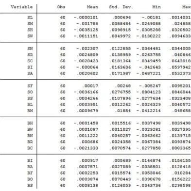
(32) J0 does not need an assumption of normally distributed errors but is only asymptotically valid. In addition, the average intercept, the average adjusted R2, the average standard error of the intercepts, the average absolute value of the intercepts and the sharpe ratio of the intercepts are also calculated. The GRS statistic uses excess returns (returns in excess of the risk-free rate) (GIBBONS, ROSS and SHANKEN, 1989).. 4 Model Results Monthly returns for each of the twenty-four portfolios were calculated. Summary statistics show that, for the twelve portfolios constructed with “Small” companies, 66% had negative mean returns. For the “Big” company portfolios, 83% had positive returns. This already seems to point to the relevance of the “Size” factor in Brazil, which will be formally tested further. The table below shows summary statistics for the return of all twenty-four portfolios, including the mean, standard deviation, and minimum and maximum values. Table 5: Portfolio Summary Statistics. The portfolios were then grouped into the ten sub-factors that will compose the zero-netinvestment factors. For size, as was shown previously, the return of the “Small” sub-factor was indeed negative, while the “Big” sub-factor was positive, showing that in Brazil the company size does attract a value premium. Nevertheless, it is relevant to note that this 32.

(33) contradicts the pattern found in the U.S. market, where empirical evidence points out that small firms should have higher excess returns in order to compensate investors for risk (F. FAMA and R. FRENCH, 1993). A possible explanation as to why this is inverted in Brazil is that in periods of high risk-aversion, such as the one analyzed, there is a generalized capital outflow from the country and smaller stocks are the most affected, losing significant value in these market troughs. For book-to-market, results showed companies with a “Low” B/M have a positive return while those with a “High B/M” have a negative return. This is contrary to what was found for the U.S. market (F. FAMA and R. FRENCH, 1993), but in line with results for Brazil found by another study (CARNEIRO MARTINS and EID JR., 2015). “High” B/M stocks are called value assets by market participants because their market values derive from assets already in place, while “Low” B/M are called growth stocks because their market values derive from expected growth in future cash flows. The market needs to assume high growth for these “Low” B/M stocks to justify the prices at which the assets trade. Simultaneously, nevertheless, a company that is distressed will see its market price fall and its B/M ratio rise. So some of the so-called value firms, with “High” B/M, may actually be distressed firms. This explains our results for Brazil, and justifies the value premium paid by the market for growth stocks. For profitability, companies with “Robust” performance have positive returns, while those with weak returns have a negative performance, in line with expectations and with another study (NOVY-MARX, 2013). Clearly, investors will pay a premium for companies with more robust results. For the investment factor, “Aggressive” companies show a positive return, while “Conservative” companies show a negative mean return. The local market pays a premium for companies that have a stronger, more aggressive investment policy. This is the opposite of what was found by other studies. Titman, Wei and Xie found that “Aggressive” companies end up having negative adjusted future returns possibly because investors tend to react negatively to empire building attitudes by managers (TITMAN, WEI and XIE, 2004). In Brazil this does not seem to be the case for this time period. For our new added factor, Governance, both companies with “Strong” and “Fragile” governance have positive returns. Nevertheless, “Strong” governance companies have a significantly higher mean return, which coincides with our expectations and shows a premium is paid for better governance. 33.

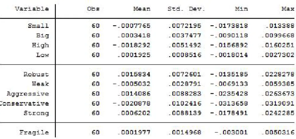
(34) The table below shows summary statistics for the return of all 10 sub-factors, including the mean, standard deviation, and minimum and maximum values. Table 6: Sub-factor Summary Statistics. Taking the analysis a step further and taking the sub-factors to build the zero-net-investment factors we find more interesting results. Most factors have negative returns, as seen in Table 7, below, that shows summary statistics for the factors, including the mean, standard deviation, and minimum and maximum values. The Rm-Rf market factor has a negative mean return. This is explained by the negative performance of the Brazilian stock market in previous years, which has indeed had very weak results caused by the macroeconomic and political turmoil of the period under analysis. For the size factor, SMB, mean return is negative. This follows our observation that the market in Brazil pays a premium for “Big” companies. Results showed that “Small” companies have a negative return, while “Big” companies have a positive return, resulting in a negative return for the SMB factor. For the value (book-to-market) factor, HML, mean return is also negative. This is in-line with our previous observations that the market pays a premium for growth stocks ("Low B/M"). Data showed that companies with a “High” B/M have a negative return while those with a “Low B/M” have a positive return, therefore justifying a negative return for the HML factor. Regarding investment, measured by the RMW factor, mean return is positive, in line with expectations that investors will pay a premium for companies with more robust results.. 34.

(35) As for investment, measured by the CMA factor, mean return is negative. We previously saw that the local market pays a premium for companies that have a stronger, more aggressive investment policy, resulting in the negative mean return. For our new factor, governance, measured by SMF, mean return is positive, according to the expectation that the market will pay a premium for stronger over more fragile governance. Nevertheless, it is important to point out the very small magnitude of the mean return of the SMF factor. Albeit being relevant, market users of this model will have to evaluate if the costs of building the governance factor justify the small absolute mean returns it delivers. Interestingly, the herding factor was also analyzed and shows a mean positive return when herding is present. Considering that herding behavior attributes price variations to the influence of herds of investors, this agrees with expectations that for a less rational market, whatever variation of market prices would be directly and positively (and not inversely) augmented by herding. Table 7: Factor Summary Statistics. An additional analysis was made between the factors before performing the regressions. The correlation between the factors was analyzed, as summarized in the table below. Table 8: Correlation of factors. 35.

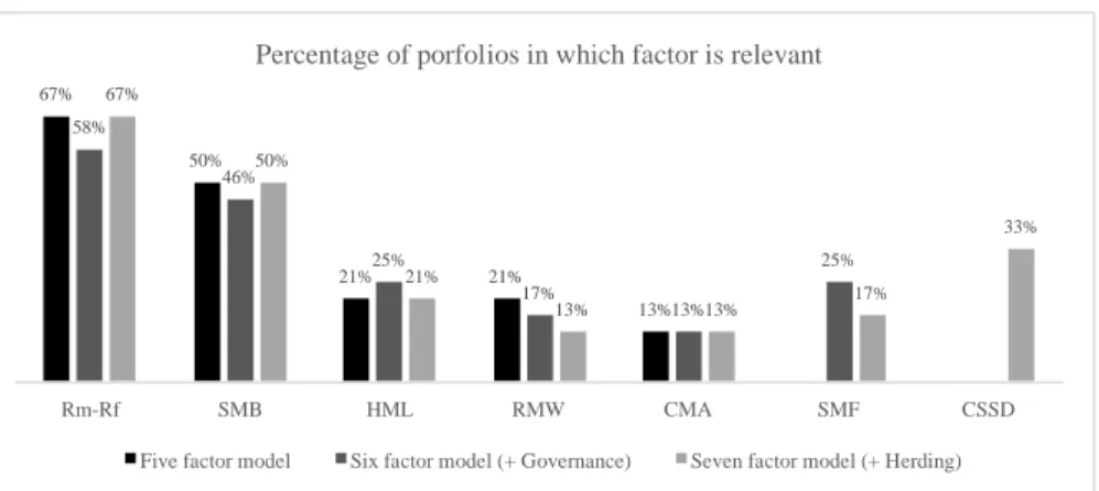
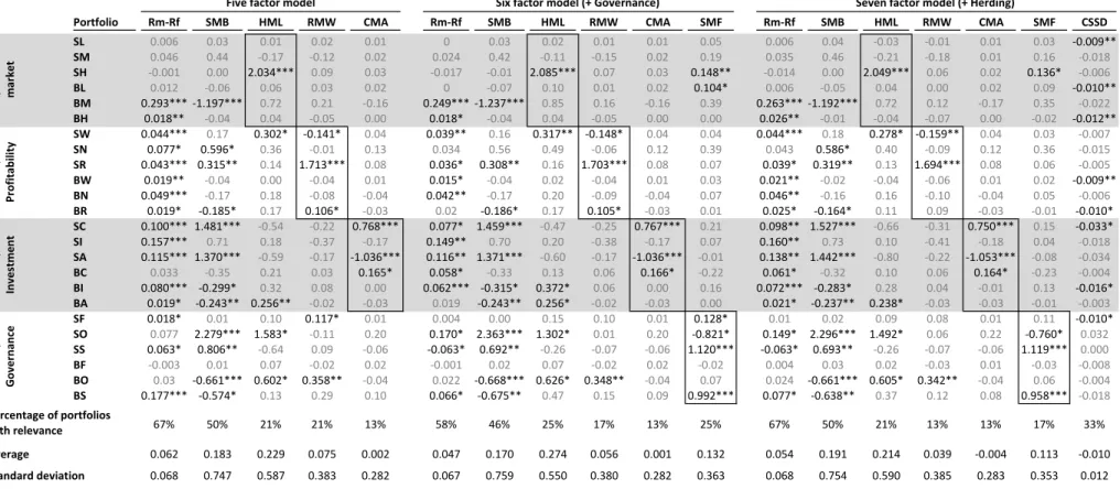
(36) The market risk premium, Rm-Rf, seems to correlate with some of the other factors, such as SMF and HML. SMB also correlates with HML. They all present correlations close too r higher than 0.6, which is significant and could create redundancy in the model. In Appendix D – Time Series for the Seven Factors, the factors are plotted in graphs to better visualize the movements of the factors over time. Moreover, in page 39, we test the models without HML to see if HML is redundant, as was the case in a previous study (F. FAMA and R. FRENCH, 2015). With portfolio returns and factors computed for each one of the 60 months of data, an ordinary least squares regression was made for each one of portfolios versus the original five factors, resulting in a total of 24 regressions. This was repeated adding the governance additional factor and then repeated again adding governance and herding factors. The detailed results of the 72 regressions can be seen in Appendix B – Detailed Outputs of Regressions. Table 10: Factor Relevance Analysis, seen in the following page, summarizes the coefficients of the regressions as well as their significance, shown with one asterisk for p-values lower than 0.05, two asterisks for p-values lower than 0.01 and three asterisks for p-values lower than 0.001. For each one of the three models tested (five-factor, six-factor and seven-factor) and for each factor, it was verified in how many of the 24 portfolios the factor is significant. The graph below summarizes the findings. Graph 9: Factor Relevance Summary Percentage of porfolios in which factor is relevant 67%. 67%. 58% 50% 50% 46% 33% 25% 21% 21%. Rm-Rf. SMB Five factor model. HML. 25%. 21% 17% 13%. 13%13%13%. RMW. CMA. Six factor model (+ Governance). 17%. SMF. CSSD. Seven factor model (+ Herding). The most relevant factors are the market factor, Rm-Rf, and size (SMB). Value (HML), profitability (RMW) and investment (CMA) were relevant in fewer portfolios. The new governance and herding factors are more relevant than factors such as CMA and RMW. It is interesting to note that for HML, RMW, CMA and SMF, each one is more relevant in the respective portfolios that include their factor, as shown by the outlined boxes in Table 10. 36.

(37) Table 10: Factor Relevance Analysis Five factor model Rm-Rf. SMB. HML. 0.006 0.046 -0.001 0.012 0.293*** 0.018** 0.044*** 0.077* 0.043*** 0.019** 0.049*** 0.019* 0.100*** 0.157*** 0.115*** 0.033 0.080*** 0.019* 0.018* 0.077 0.063* -0.003 0.03 0.177***. 0.03 0.44 0.00 -0.06 -1.197*** -0.04 0.17 0.596* 0.315** -0.04 -0.17 -0.185* 1.481*** 0.71 1.370*** -0.35 -0.299* -0.243** 0.01 2.279*** 0.806** 0.01 -0.661*** -0.574*. 0.01 -0.17 2.034*** 0.06 0.72 0.04 0.302* 0.36 0.14 0.00 0.18 0.17 -0.54 0.18 -0.59 0.21 0.32 0.256** 0.10 1.583* -0.64 0.07 0.602* 0.13. Percentage of portfolios with relevance. 67%. 50%. 21%. 21%. Average. 0.062. 0.183. 0.229. Standard deviation. 0.068. 0.747. 0.587. Size / Governance. Size / Investment. Size / Profitability. Size / Book-tomarket. Portfolio SL SM SH BL BM BH SW SN SR BW BN BR SC SI SA BC BI BA SF SO SS BF BO BS. * p<0.05, ** p<0.01, *** p<0.001. 37. RMW. Six factor model (+ Governance) CMA. Rm-Rf. SMB. HML. 0 0.024 -0.017 0 0.249*** 0.018* 0.039** 0.034 0.036* 0.015* 0.042** 0.02 0.077* 0.149** 0.116** 0.058* 0.062*** 0.019 0.004 0.170* -0.063* -0.001 0.022 0.066*. 0.03 0.42 -0.01 -0.07 -1.237*** -0.04 0.16 0.56 0.308** -0.04 -0.17 -0.186* 1.459*** 0.70 1.371*** -0.33 -0.315* -0.243** 0.00 2.363*** 0.692** 0.02 -0.668*** -0.675**. 0.02 -0.11 2.085*** 0.10 0.85 0.04 0.317** 0.49 0.16 0.02 0.20 0.17 -0.47 0.20 -0.60 0.13 0.372* 0.256* 0.15 1.302* -0.26 0.07 0.626* 0.47. 13%. 58%. 46%. 25%. 17%. 13%. 0.075. 0.002. 0.047. 0.170. 0.274. 0.056. 0.383. 0.282. 0.067. 0.759. 0.550. 0.380. 0.02 0.01 -0.12 0.02 0.09 0.03 0.03 0.02 0.21 -0.16 -0.05 0.00 -0.141* 0.04 -0.01 0.13 1.713*** 0.08 -0.04 0.01 -0.08 -0.04 0.106* -0.03 -0.22 0.768*** -0.37 -0.17 -0.17 -1.036*** 0.03 0.165* 0.08 0.00 -0.02 -0.03 0.117* 0.01 -0.11 0.20 0.09 -0.06 -0.02 0.02 0.358** -0.04 0.29 0.10. RMW. CMA. Seven factor model (+ Herding) SMF. Rm-Rf. SMB. 0.006 0.035 -0.014 0.006 0.263*** 0.026** 0.044*** 0.043 0.039* 0.021** 0.046** 0.025* 0.098** 0.160** 0.138** 0.061* 0.072*** 0.021* 0.01 0.149* -0.063* 0.004 0.024 0.077*. 0.04 0.46 0.00 -0.05 -1.192*** -0.01 0.18 0.586* 0.319** -0.02 -0.16 -0.164* 1.527*** 0.73 1.442*** -0.32 -0.283* -0.237** 0.02 2.296*** 0.693** 0.03 -0.661*** -0.638**. 25%. 67%. 50%. 21%. 13%. 13%. 17%. 33%. 0.001. 0.132. 0.054. 0.191. 0.214. 0.039. -0.004. 0.113. -0.010. 0.282. 0.363. 0.068. 0.754. 0.590. 0.385. 0.283. 0.353. 0.012. 0.01 0.01 0.05 -0.15 0.02 0.19 0.07 0.03 0.148** 0.01 0.02 0.104* 0.16 -0.16 0.39 -0.05 0.00 0.00 -0.148* 0.04 0.04 -0.06 0.12 0.39 1.703*** 0.08 0.07 -0.04 0.01 0.03 -0.09 -0.04 0.07 0.105* -0.03 0.01 -0.25 0.767*** 0.21 -0.38 -0.17 0.07 -0.17 -1.036*** -0.01 0.06 0.166* -0.22 0.06 0.00 0.16 -0.02 -0.03 0.00 0.10 0.01 0.128* 0.01 0.20 -0.821* -0.07 -0.06 1.120*** -0.02 0.02 -0.02 0.348** -0.04 0.07 0.15 0.09 0.992***. HML. RMW. CMA. SMF. -0.03 -0.01 0.01 0.03 -0.21 -0.18 0.01 0.16 2.049*** 0.06 0.02 0.136* 0.04 0.00 0.02 0.09 0.72 0.12 -0.17 0.35 -0.04 -0.07 0.00 -0.02 0.278* -0.159** 0.04 0.03 0.40 -0.09 0.12 0.36 0.13 1.694*** 0.08 0.06 -0.04 -0.06 0.01 0.02 0.16 -0.10 -0.04 0.05 0.11 0.09 -0.03 -0.01 -0.66 -0.31 0.750*** 0.15 0.10 -0.41 -0.18 0.04 -0.80 -0.22 -1.053*** -0.08 0.10 0.06 0.164* -0.23 0.28 0.04 -0.01 0.13 0.238* -0.03 -0.03 -0.01 0.09 0.08 0.01 0.11 1.492* 0.06 0.22 -0.760* -0.26 -0.07 -0.06 1.119*** 0.02 -0.03 0.01 -0.03 0.605* 0.342** -0.04 0.06 0.37 0.12 0.08 0.958***. CSSD -0.009** -0.018 -0.006 -0.010** -0.022 -0.012** -0.007 -0.015 -0.005 -0.009** -0.006 -0.010* -0.033* -0.018 -0.034 -0.004 -0.016* -0.003 -0.010* 0.032 0.000 -0.008 -0.004 -0.018.

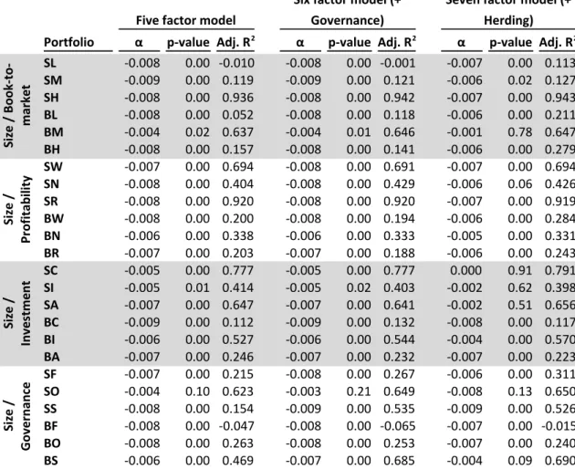
(38) In the regression, if the exposure to the factors capture all the variation in the expected returns, the intercept, alpha, should be zero for all securities and portfolios. If an asset pricing model completely captures expected returns, the intercept would be indistinguishable from zero (F. FAMA and R. FRENCH, 2015). Table 11, below, summarizes the intercept (alpha), the pvalue and the adjusted R2 for each one of the three models and 24 portfolios. In both the fivefactor and six-factor models, over 95% of portfolios have an alpha that is indistinguishable from zero. For the seven-factor model, this is the case for over 70% of portfolios.. Size / Governance. Size / Investment. Size / Profitability. Size / Book-tomarket. Table 11: Consolidated Alpha Analysis. Portfolio SL SM SH BL BM BH SW SN SR BW BN BR SC SI SA BC BI BA SF SO SS BF BO BS. Five factor model. Six factor model (+ Governance). Seven factor model (+ Herding). α p-value Adj. R 2 -0.008 0.00 -0.010 -0.009 0.00 0.119 -0.008 0.00 0.936 -0.008 0.00 0.052 -0.004 0.02 0.637 -0.008 0.00 0.157 -0.007 0.00 0.694 -0.008 0.00 0.404 -0.008 0.00 0.920 -0.008 0.00 0.200 -0.006 0.00 0.338 -0.007 0.00 0.203 -0.005 0.00 0.777 -0.005 0.01 0.414 -0.007 0.00 0.647 -0.009 0.00 0.112 -0.006 0.00 0.527 -0.007 0.00 0.246 -0.007 0.00 0.215 -0.004 0.10 0.623 -0.008 0.00 0.154 -0.008 0.00 -0.047 -0.008 0.00 0.263 -0.006 0.00 0.469. α p-value Adj. R 2 -0.008 0.00 -0.001 -0.009 0.00 0.121 -0.008 0.00 0.942 -0.008 0.00 0.118 -0.004 0.01 0.646 -0.008 0.00 0.141 -0.008 0.00 0.691 -0.008 0.00 0.429 -0.008 0.00 0.920 -0.008 0.00 0.194 -0.006 0.00 0.333 -0.007 0.00 0.188 -0.005 0.00 0.777 -0.005 0.02 0.403 -0.007 0.00 0.641 -0.009 0.00 0.132 -0.006 0.00 0.544 -0.007 0.00 0.232 -0.008 0.00 0.267 -0.003 0.21 0.649 -0.009 0.00 0.535 -0.008 0.00 -0.065 -0.008 0.00 0.253 -0.007 0.00 0.685. α p-value Adj. R 2 -0.007 0.00 0.113 -0.006 0.02 0.127 -0.007 0.00 0.943 -0.006 0.00 0.211 -0.001 0.78 0.647 -0.006 0.00 0.279 -0.007 0.00 0.694 -0.006 0.06 0.426 -0.007 0.00 0.919 -0.006 0.00 0.284 -0.005 0.00 0.331 -0.006 0.00 0.243 0.000 0.91 0.791 -0.002 0.62 0.398 -0.002 0.51 0.656 -0.008 0.00 0.117 -0.004 0.00 0.570 -0.007 0.00 0.223 -0.006 0.00 0.311 -0.008 0.13 0.650 -0.009 0.00 0.526 -0.007 0.00 -0.015 -0.007 0.00 0.240 -0.004 0.09 0.690. The above statistics test the intercepts for each portfolio. In order to test for the null intercept hypothesis for combinations of portfolios and factors, we can use the GRS statistic. Table 12, below, shows the results of the GRS statistic. It can be seen that the intercept is jointly indistinguishable from zero for the combinations of factors and portfolios. 38.

(39) Table 12: GRS Statistics. Seven factor model Six factor model (+ (+ Herding) Governance). Five factor model. J1 Mean α Test statistic P-value Mean adj. R2 Mean SE Mean abs. val. α Sharpe ratio Mean α Test statistic P-value Mean adj. R2 Mean SE Mean abs. val. α Sharpe ratio Mean α Test statistic P-value Mean adj. R2 Mean SE Mean abs. val. α Sharpe ratio. -0.007038 33.824 0.000000 0.377023 0.000876 0.007038 5.709925 -0.007197 31.604 0.000000 0.407295 0.000855 0.007197 5.706177 -0.005633 5.550 0.000011 0.432140 0.001863 0.005633 5.314918. J0 -0.007038 1571.183 0.000000 0.377023 0.000876 0.007038 0.000000 -0.007197 1516.998 0.000000 0.407295 0.000855 0.007197 0.000000 -0.005633 275.576 0.000000 0.432140 0.001863 0.005633 0.000000. Before moving on to the conclusions, one final analysis could be relevant. In Fama and French’s seminal paper, the value factor of their three-factor model became redundant for describing average returns in the sample they examined (F. FAMA and R. FRENCH, 2015). With this inspiration, regressions on the three models were run again, but this time without the HML factor. Once again, if an asset pricing model completely captures expected returns, the intercept would be indistinguishable from zero (F. FAMA and R. FRENCH, 2015). Table 13, below, summarizes the intercept (alpha), the p-value and the adjusted R2 for each one of the three models and 18 portfolios. In the original model (but now without HML), 100% of the portfolios have an alpha that is indistinguishable from zero (versus over 95% with HML). When we add governance, the model without HML shows that slightly under 95% of portfolios have an alpha indistinguishable from zero (versus over 95% with HML). Finally, when herding is added, the number of portfolios with an alpha that is indistinguishable from zero falls to 67% (versus over 70% with HML). 39.

(40) Table 13: Consolidated Alpha Analysis without HML. Size / Governance. Size / Investment. Size / Profitability. Original model Portfolio SW SN SR BW BN BR SC SI SA BC BI BA SF SO SS BF BO BS. + Governance. α p-value Adj. R -0.008 0.00 0.660 -0.008 0.00 0.405 -0.008 0.00 0.921 -0.008 0.00 0.215 -0.006 0.00 0.331 -0.008 0.00 0.175 -0.005 0.00 0.770 -0.005 -0.01 0.423 -0.007 0.00 0.639 -0.01 0.00 0.118 -0.006 0.00 0.503 -0.007 0.00 0.159 -0.008 0.00 0.215 -0.006 -0.03 0.590 -0.007 0.00 0.127 -0.008 0.00 -0.040 -0.008 0.00 0.189 -0.006 0.00 0.477. 2. + Herding. α p-value Adj. R -0.008 0.00 0.654 -0.008 0.00 0.422 -0.008 0.00 0.920 -0.008 0.00 0.209 -0.006 0.00 0.322 -0.008 0.00 0.161 -0.005 0.00 0.774 -0.005 -0.01 0.412 -0.007 0.00 0.633 -0.009 0.00 0.144 -0.007 0.00 0.509 -0.007 0.00 0.148 -0.008 0.00 0.253 -0.004 -0.10 0.629 -0.009 0.00 0.537 -0.008 0.00 -0.055 -0.008 0.00 0.174 -0.007 0.00 0.675. 2. α p-value Adj. R 2 -0.006 0.00 0.668 -0.005 -0.09 0.425 -0.007 0.00 0.920 -0.006 0.00 0.293 -0.005 0.00 0.329 -0.006 0.00 0.241 -0.001 -0.69 0.780 -0.002 -0.64 0.409 -0.003 -0.35 0.638 -0.008 0.00 0.132 -0.004 -0.01 0.555 -0.006 0.00 0.157 -0.006 0.00 0.314 -0.006 -0.25 0.623 -0.009 0.00 0.529 -0.007 0.00 0.004 -0.007 0.00 0.173 -0.004 -0.13 0.686. The differences in adjusted R2 for all three models are not significant when comparing the models with HML to those without HML. For the original five-factor model, our results are compatible to those found by Fama and French (F. FAMA and R. FRENCH, 2015). The value factor becomes in fact redundant. Nevertheless, when we add governance and then herding, we do indeed lose some significance, since the percentage of portfolios in which alpha is indistinguishable from zero decreases.. 5 Conclusions The objective of this thesis, in broad terms, was to build upon previous work and investigate the risk-return relationships of stocks not explained by the CAPM. In other words, the proposal was to scrutinize the effect of other variables other than the market factor (Rm-Rf) on stock returns. More specifically, the objective was to complement Fama and French´s five original factors with two new factors that could prove to have some significance in explaining stock returns (F. FAMA and R. FRENCH, 2015). This is a significant contribution in the sense that that current models have not yet been able to completely reduce alpha to zero. Regarding the new factors, uncertainties about the efficiency of the market suggested that 40.