Performance measurement models and their influence on net fundraising of investment funds

(1)

DOI: 10.1590/1808-057x201805330

Original Article

Performance measurement models and their influence on net

fundraising of investment funds

Anderson Rocha de J. Fernandes1 https://orcid.org/0000-0003-3323-1967

Email: andersonr@ufmg.com

Simone Evangelista Fonseca2

Email: sissafonseca@adm.grad.ufmg.br

Robert Aldo Iquiapaza3

https://orcid.org/0000-0003-1657-2823

Email: rbali@ufmg.br

1_{Universidade Federal de Minas Gerais, Faculdade de Ciências Econômicas, Centro de Desenvolvimento e Planejamento Regional, Belo}

Horizonte, MG, Brazil

2_{Universidade Federal de Minas Gerais, Faculdade de Ciências Econômicas, Departamento de Ciências Administrativas, Belo Horizonte, MG,}

Brazil

3_{Universidade Federal de Minas Gerais, Faculdade de Ciências Econômicas, Centro de Pós-Graduação e Pesquisas em Administração, Belo}

Horizonte, MG, Brazil

Received on 02.21.2017 – Desk acceptance on 05.18.2017 – 4th_{version approved on 11.13.2017 – Ahead of print on 06.18.2018} Associate Editor: Fernanda Finotti Cordeiro Perobelli

ABSTRACT

This article aims to analyze the relation between third- and fourth-order conditions and risk factors and their adequacy to return, performance, and net fundraising. The factors used to determine fund performance and, consequently, their relation with fundraising are: market return, size, book-to-market, profitability, investment, co-skewness, and co-kurtosis. The funds constituting the sample are those classified as Free Stocks (within the period from April 2001 to April 2015). Methodologically, this study has two phases. The first one refers to estimating the parameters that represent fund sensitivity to the factors and the comparison of the capital asset pricing models (CAPM), French-Carhart 4-factor (FFC), Fama-French 5-factor (FF5), Fama-Fama-French 5-factor with momentum (FF5M), added or not with co-moments, by means of the fixed-effects procedure. The second one deals with verifying the relation between performance and net fundraising. The models were reestimated through moving time windows, so that the alpha calculated on each of them represented fund performance within the immediately subsequent period. We also estimated the relation fundraising-performance through cross-section regressions, with rates and age as control variables. The results showed that the co-skewness and co-kurtosis coefficients are not that relevant for determining performance and net fundraising of investment funds. Among the risk factors, market, size, and momentum are the significant parameters for fund returns. The FFC and FF5M models are those with greater explanatory power regarding return specification. There is also evidence of convexity in the relation between performance and fundraising.

Keywords: investment funds, performance, net fundraising, asset pricing models, market risk.

Correspondence address

Anderson Rocha de J. Fernandes

Universidade Federal de Minas Gerais, Faculdade de Ciências Econômicas, Centro de Desenvolvimento e Planejamento Regional

(2)

1. INTRODUCTION

Investment fund performance may be measured through mathematical models that relate risk factors to their returns. This performance evaluation procedure consists in estimating performance through variables that represent risks inherent to assets in the capital markets (Babalos, Mamatzakis & Matousek, 2015).

Among the criteria that drive the choice to form these portfolios, it is worth highlighting the constitution of an optimal relation between risk and return. According to Markowitz (1952), investors must diversify their investments by looking at the profitability and variability of financial assets belonging to the portfolio.

Portfolio selection analysis considers only the first two statistical moments (mean value and variance), based on the assumption that financial asset returns follow a normal distribution (Scott & Horvath, 1980). With such a premise, several pricing models have been developed, in order to better understand how return is impacted by the existence of risk.

Among the procedures, we highlight the capital asset pricing model(CAPM), which relates asset expected return exclusively to its market risk (Sharpe, 1964). Due to CAPM inconsistencies, resulting from the risk factor unity, models have been developed considering other factors. The variables used in this study are those defined by Fama and French (1993), size and book-to-market; by Carhart (1997), momentum, with the Fama-French-Carhart 4-factor model (FFC); and by Fama and French (2015), profitability and investment, with the Fama-French 5-factor model (FF5).

It is also argued that return behavior may not show the characteristics of a normal distribution, a fact that makes it worth evaluating higher moments, in asset pricing (Hong, Tu & Zhou, 2007). The explanatory power of the third- and fourth-order moments is a theme addressed by Kostakis, Muhammad and Siganos (2012), which analyze stocks on the London Stock Exchange. Such variables have explanatory potential regarding other factors: covariance,

size, book-to-market, and momentum.

Brazilian stock investment funds classified as Free Stocks are evaluated in this study. A fund is an alternative for collective investment of financial resources where individuals acquire quotas proportional to their allocations (Associação Brasileira das Entidades dos Mercados Financeiro e de Capitais – ANBIMA, 2015; Fonseca, Bressan, Iquiapaza & Guerra, 2007).

Investment fund performance is associated with net fundraising (resource attractiveness degree). According to Chevalier and Ellison (1997), Ippolito (1992), and Sirri and Tufano (1998), funds with higher returns also have higher levels of net contribution to their equity: investors allocate their funds to better performing portfolios, expecting it to be repeated. Also, net fundraising reflects the flow of resources in the investment fund industry (Iquiapaza, Barbosa, Amaral & Bressan, 2008).

Thus, this study aims to grasp the influence of comoments on fund performance, as well as their relation with risk factors in pricing models. The relationship between performance and net fundraising is also investigated.

In an analysis similar to that conducted by Barber, Huang and Odean (2016), the objective is grasping the response of resource flows of Brazilian funds to their performance, measured through the pricing model intercepts, a measurement named as Jensen’s alpha. The research also aims to verify how risk factors – market, size, book-to-market, profitability, investment, momentum, and third- and fourth-order conditions – may influence fundraising in Brazilian investment portfolios.

(3)

2. THEORETICAL FRAMEWORK

2.1 Pricing Models and Inclusion of Statistical Moments

Pricing models have been developed with the assumption that return and risk are enough for the portfolio selection and evaluation process. The CAPM, as proposed by Lintner (1965), Mossin (1966), and Sharpe (1964), represents a linear relation between a stock return and its risk premium. The model assumptions are homogeneous expectations and the existence of a risk-free asset. The CAPM is presented in equation 1:

where R_iis the expected return on the stock i, R_fis the risk-free rate, R_M is the market portfolio return, and β_iis the systemic risk component of stock i.

Diversification reduces a part of a portfolio’s risk. Therefore, according to Sharpe (1964), only the remaining component is important so that its expected return can be established. Such a component, represented by β_i in equation 1, measures the degree to which the returns of asset i move along with the market portfolio return. Therefore, the CAPM is an extension of the mean-variance environment, where risk is represented in equation 2:

Black, Jensen and Scholes (1972) and Lintner (1965) listed some assumptions that underpin the CAPM and also represent its limitations: (i) all investors can lend and borrow at the risk-free rate, R_f; (ii) absence of transaction costs and taxes; (iii) risk aversion and utility maximization in the mean-variance dimension; and (iv) assets are infinitely fractable, i.e. they can be traded in any amounts.

Among the models with multiple risk factors, we highlight that developed by Fama and French (1993).

According to the authors, firms’ size and firms’ book-to-market complement book-to-market risk, in terms of explaining financial security returns. Investors’ perception of companies’ performance depends on the magnitude of their book-to-market ratio value, and size is directly related to profitability.

The risk factors related to these two measurements are based on the difference between the returns of portfolios formed by stocks with high book-to-market values and low book-to-market values, forming the high-minus-low (HML) factor. The small-minus-big (SMB) construct stems from the difference between portfolios formed by small firm stocks and portfolios formed by big firm stocks, representing the size factor. The 3-factor Fama-French (FF3) model is represented in equation 3:

where α_i is the intercept, β_i is the systemic risk, s_i is sensitivity to the size factor, SMB is the size factor, h_i

is sensitivity to the book-to-market factor, HML is the book-to-market factor, and is the random error.

According to Carhart (1997), the variables described in FF3 are significant, but they do not explain the persistence of portfolio (under)performance. Thus, the author included a fourth factor that attempts to capture such an anomaly, named as “momentum effect.” The momentum, described by Jegadeesh and Titman (1993), is the continuity of the results of assets for a certain period, that is, the maintenance, in the future, of past, positive or negative returns. Carhart (1997) includes it in FF3, forming the FFC model for fund evaluation, represented in equation 4. Like SMB and HML, MOM consists in the difference between portfolio return of winning stocks and another one, of losing stocks:

1

𝑅𝑅

𝑖𝑖

= 𝑅𝑅

𝑓𝑓

+ 𝛽𝛽

𝑖𝑖

(𝑅𝑅

𝑀𝑀

− 𝑅𝑅

𝑓𝑓

)

𝛽𝛽

𝑖𝑖

=

𝑐𝑐𝑐𝑐𝑐𝑐(𝑅𝑅𝑖𝑖, 𝑅𝑅𝑀𝑀

_{𝑐𝑐𝑣𝑣𝑣𝑣(𝑅𝑅}

)

𝑀𝑀

)

𝑅𝑅𝑖𝑖

− 𝑅𝑅𝑓𝑓

= 𝛼𝛼𝑖𝑖

+ 𝛽𝛽𝑖𝑖

(𝑅𝑅𝑀𝑀

− 𝑅𝑅𝑓𝑓) + 𝑠𝑠𝑖𝑖𝑆𝑆𝑆𝑆𝑆𝑆 + ℎ𝑖𝑖

𝐻𝐻𝑆𝑆𝐻𝐻 + 𝜀𝜀𝑖𝑖

(4)

where m_i is the coefficient of sensitivity to the momentum factor and MOM is the momentum factor.

Novy-Marx (2013) has shown that firms’ ability to generate profits is associated with average returns on their securities, explaining them as much as the book-to-maket. Aharoni, Grundy and Zeng (2013) related investment to stock returns, also turning this into a major variable.

Fama and French (2015), when reanalysing the FF3

model, have seen that such variables could be relevant to asset pricing, addressing anomalies that challenged the FF3. Thus, they have developed proxies for profitability and investment and added them to the model, since expectations regarding a company relate to its profitability and ability to invest. The FF5 model is represented in equation 5:

where RMW_t (robust-minus-weak) is the profitability factor, r_i is sensitivity to RMW_t, CMA_t ( conservative-minus-aggressive) is the investment factor and c_i is the effect of CMA_ton returns. Details on factor construction are discussed in section 3.2, subsection risk factors and portfolios.

Chiah, Chai, Zhong and Li (2016) tested the FF5 model for the Australian market, comparing it to the FF3 and the FFC. The results showed that the profitability and investment factors lead the FF5 to show a better explanatory power.

It is worth specifying how a pricing model can include and represent the statistical moments. According to Kraus and Litzenberger (1976), such a model is a market equilibrium equation that may be described linearly, considering the excess returns of asset i in relation to a risk-free asset (R_f), as highlighted in equation 6:

where λ_i (i = 1,..., 3) represents the increase through market risk, systemic skewness and systemic kurtosis, and β_i, γ_iand δ_iare the systemic risk, co-skewness and co-kurtosis, respectively.

As these are comoments (i.e. statistical moments in relation to some reference variable), the coefficients –

represented in equations 7, 8, and 9 – measure the sensitivity in terms of variance, skewness, and kurtosis of return on the asset i in relation to the market portfolio M. The coefficient β_i is the systemic risk defined in equation 2.

The parameters β_i, γ_iand δ_i represent the contribution in variance, skewness, and kurtosis of the asset i for the market portfolio. The magnitudes of changes on the returns of i, given the variations in variance, skewness, or kurtosis of the market portfolio R_M, respectively (Ceretta, Catarina & Muller, 2007).

Assuming that equation 6 is valid for all investors,

λ₁, λ₂ and λ₃should be interpreted as market prices for systemic risk (β), for co-skewness (γ) and co-kurtosis (δ), respectively (Fang & Lai, 1997; Kraus & Litzenberger, 1976). Proxies for covariance, skewness, and co-kurtosis may be defined and the model in equation 6 may be rewritten:

Equation 10 depicts the analysis of financial asset behavior from variance, systemic skewness, and systemic kurtosis (comoments) in relation to returns on the market portfolio R_M. The incorporation of variables that expand the mean-variance space is useful to understand changes in asset returns when characteristics of their probability distribution are considered.

2.2 Funds’ Net Fundraising and their Relation to Performance

Investment fund performance is related to capacity to attract resources by increasing the number of quota holders (Sirri & Tufano, 1998). The latter invest in funds evaluating their past results, which form expectations

𝑅𝑅𝑖𝑖𝑖𝑖− 𝑅𝑅𝑓𝑓𝑖𝑖 = 𝛼𝛼𝑖𝑖+ 𝛽𝛽𝑖𝑖(𝑅𝑅𝑀𝑀𝑖𝑖− 𝑅𝑅𝑓𝑓) + 𝑠𝑠𝑖𝑖𝑆𝑆𝑆𝑆𝑆𝑆𝑖𝑖+ ℎ𝑖𝑖𝐻𝐻𝑆𝑆𝐻𝐻𝑖𝑖+ 𝑟𝑟𝑖𝑖𝑅𝑅𝑆𝑆𝑅𝑅𝑖𝑖+ 𝑐𝑐𝑖𝑖𝐶𝐶𝑆𝑆𝐶𝐶𝑖𝑖+

𝜀𝜀

𝑖𝑖𝑖𝑖 5

𝐸𝐸(𝑅𝑅

𝑖𝑖) − 𝑅𝑅𝑓𝑓

= 𝜆𝜆

1

𝛽𝛽

𝑖𝑖

+ 𝜆𝜆

2

𝛾𝛾

𝑖𝑖

+ 𝜆𝜆

3

𝛿𝛿

𝑖𝑖 6

𝛽𝛽𝑖𝑖=𝐸𝐸[(𝑅𝑅_{𝐸𝐸[(𝑅𝑅}𝑖𝑖− 𝑅𝑅̅𝑖𝑖)(𝑅𝑅𝑀𝑀− 𝑅𝑅̅𝑀𝑀)] 𝑀𝑀− 𝑅𝑅̅𝑀𝑀)2]

𝛾𝛾𝑖𝑖=𝐸𝐸[(𝑅𝑅𝑖𝑖− 𝑅𝑅̅𝑖𝑖)(𝑅𝑅𝑀𝑀− 𝑅𝑅̅𝑀𝑀) 2_]

𝐸𝐸[(𝑅𝑅𝑀𝑀− 𝑅𝑅̅𝑀𝑀)3]

𝑀𝑀

− 𝐸𝐸(𝑅𝑅

𝑀𝑀

))

3 10

8

(5)

about the future behavior of quotas. There is also, according to Warther (1995), the fact that flows also

exert influence on prices, therefore, on return.

Net fundraising may be defined as the difference between the new values added to the fund’s equity and full redemption within a given period. It is assumed that a rational investor allocates funds in portfolios that optimize risk and return, contributing to the fundraising composition (Sirri & Tufano, 1998). We may say that portfolio fundraising depends on numerous factors, such as net equity, age, rates, and performance.

Sirri and Tufano (1998) associate the investment fund fundraising level to its lagged returns, motivated by the assumption that portfolios that had positive past performance tend to attract more resources. However, this association shows convexity. Investors’ responses to negative past returns are different from those provided to people who achieved positive returns. According to the authors, the largest allocations are disproportionately distributed to funds with the best past performance, i.e. the fundraising-performance relation is asymmetric. The results of that study show that fundraising is also linked to size and administration fees. Ippolito (1992) also shows

the existence of an asymmetrical relation between fund’s portfolio allocation and its performance.

Fundraising determinants are also addressed by Ferreira, Keswani, Miguel and Ramos (2012), who list differences of the fund industries in various countries. The study found that investors in developed countries are more sophisticated, as they are able to face lower operating costs due to the broad investment alternatives. The authors argue that the greater investors’ sophistication, the lower convexity in the fundraising-performance relation.

Barber et al. (2016) related risk factors to mutual fund’s fundraising, in an attempt to establish the most adequate performance measurement for predicting funds’ resource flows. The models used by the authors were: market-adjusted returns, CAPM, FF3, FFC, 7 factors, which includes 3 industrial variables, and 9 factors, which also aggregates profitability and investment. The study results showed that the CAPM alpha value is the best measure to estimate fundraising, and that market risk (beta) is the most frequently considered by investors when evaluating funds. Table 1 summarizes the results of studies using risk factors and higher funds’ comoments.

3. METHODOLOGICAL PROCEDURES

3.1 Sample and Data

The sample encompasses non-exclusive investment funds classified as Free Stocks. This is the category, among stock funds, which does not require a benchmark and it is also the one with the highest volume. It is worth noticing that analyses were also carried out with active BOVESPA Index (IBOVESPA) and Brazilian Index (IBrX) funds (non-reported results). Data was collected between 2001 and 2015, on a monthly basis, according to

the ANBIMA classification criteria.

Extreme observations may affect the analyses of results obtained in descriptive statistics and in regressions. Hair, Black, Anderson and Babin (2010) argue that outliers that do not represent the population must be suppressed. Thus, as they were fund return series, we eliminated from the study sample actually discrepant values of a certain fund series, i.e. returns that did not match with the quota’s value change.

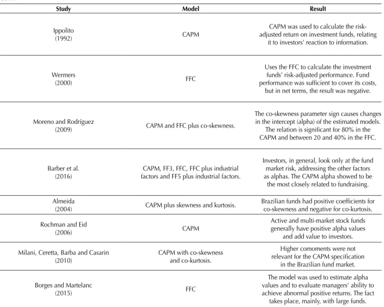
Table 1

Studies that relate funds, factors, and comoments

Study Model Result

Treynor and Mazuy (1966)

CAPM plus market timing.

Investment fund managers cannot anticipate the market. Without evidence of curvature in characteristic lines of the funds addressed,

i.e. the estimated parameter of market timing is not statistically significant.

Ang and Chua

(1979) CAPM plus skewness.

The Sharpe-Lintner-Mossin CAPM is unsatisfactory in assessing fund performance,

(6)

Study Model Result

Ippolito

(1992) CAPM

CAPM was used to calculate the risk-adjusted return on investment funds, relating

it to investors’ reaction to information.

Wermers

(2000) FFC

Uses the FFC to calculate the investment funds’ risk-adjusted performance. Fund performance was sufficient to cover its costs,

but in net terms, the result was negative.

Moreno and Rodríguez

(2009) CAPM and FFC plus co-skewness.

The co-skewness parameter sign causes changes in the intercept (alpha) of the estimated models.

The relation is significant for 80% in the CAPM and between 20 and 40% in the FFC.

Barber et al. (2016)

CAPM, FF3, FFC, FFC plus industrial factors and FF5 plus industrial factors.

Investors, in general, look only at the fund market risk, addressing the other factors as alphas. The CAPM alpha showed to be

the most closely related to fundraising.

Almeida

(2004) CAPM plus skewness and kurtosis.

Brazilian funds had positive coefficients for co-skewness and negative for co-kurtosis.

Rochman and Eid

(2006) CAPM

Active and multi-market stock funds generally have positive alpha values

and add value to investors.

Milani, Ceretta, Barba and Casarin (2010)

CAPM with co-skewness and co-kurtosis.

Higher comoments were not relevant for the CAPM specification

in the Brazilian fund market.

Borges and Martelanc

(2015) FFC

The model was used to estimate alpha values and to evaluate managers’ ability to achieve abnormal positive returns. The fact

takes place, mainly, with large funds.

CAPM= capital asset pricing model; FF3 = 3-factor Fama-French; FF5 = 5-factor Fama-French; FFC = 4-factor Fama-French-Carhart.

Source: Prepared by the authors.

Considering the interquartile range interval procedure, described by Stevenson (1981) and represented in equation 11, we used a constant k = 1.5, which represents an amplitude suggested by Stevenson (1981), so that extremely discrepant returns can be eliminated from potential database errors.

where Q₁ is the first quartile, Q₃is the third quartile, and

k is a constant equal to 1.5.

For data analysis, the funds were separated – after eliminating outliers through equation 11, according to Carhart (1997) –, in terms of their returns: from the

most profitable (P1) to the least profitable (P10), allowing a risk-adjusted performance check based on returns. We maintained in the sample funds that showed at least 12 months of returns, so that their variability could be evaluated for a certain period, avoiding survival bias.

3.2 Data Collection and Study Variables

The collection of data described in this section took place by means of the databases Quantum

®

and SI-ANBIMA. Therefore, secondary data were obtained. Data processing resorted to the software R, setting where the statistical models were both estimated and analyzed.

Data that serve as inputs to the analyzes proposed by

Table 1

Cont.

(7)

this study are the monthly fund returns. From the latter, the risk-free rate (Brazilian interbank deposit certificate – CDI) was subtracted to calculate excess returns (R_i- R_f), a dependent variable in the pricing models. The market premium (R_M - R_f) was constituted through IBOVESPA returns. Co-skewness and co-kurtosis proxies were also used in the models.

The constitution of risk factors requires data from companies traded on stock exchanges. Closing prices and monthly returns, equity value, stock market value, operating profit, and total assets were used to estimate the constructs SMB, HML, MOM, RMW and CMA. In the next subsection, we detail the construction of these factors, which are inputs for the FFC, FF5, and FF5M models.

3.2.1 Risk factors and portfolios.

The procedure used to establish the risk factors SMB,

HML, RMW, CMA and MOM is similar to that proposed by Fama and French (1993, 2015, 2016), adapted for Brazilian data. Stocks traded on the São Paulo Stock, Mercantile and Futures Exchange (BM&FBOVESPA), excluding those in the financial sector, just as Fama and French (2015) did, since these companies have specific accounting characteristics.

The relevant inputs to construct the portfolios are the companies’ market value in year t and the book-to-market ratio (dividing the stock’s equity value by its book-to-market value), whose portfolios are formed in the end of June of year t. To do so, the book-to-market value is used in the end of t-1. The proxy for profitability (OP), according to Fama and French (2015), is the operating profit free of financial expenses in the end of t-1 divided by equity in

t-1. Finally, the investment variable (Inv) in year t refers to companies’ total asset growth between years t-2 and

t-1. Portfolios based on profitability and investment are also formed in the end of June.

Following the procedure proposed by Fama and French (1993), stocks were classified according to size – small (S

– small market value) and big (B – big market value) in relation to the median of their market value. Subsequently, percentiles of the book-to-market index were used to divide them into high (H – > 70), neutral (N – between 30 and 70), and low (L – <30). Thus, 6 portfolios that relate size to book-to-market were formed (SH, SN, SL, BH, BN

and BL). According to Fama and French (2015), the factor

SMB_BM is the average of returns on the 3 small portfolios subtracted of average returns on the 3 big portfolios in relation to the book-to-market. The results of SMB_BM were used in the FFC model in this study, since it does not take into account profitability and investment.

Unlike the 1993 study, Fama and French (2015) also

have the variables SMB_OP and SMB_Inv, which are ways to verify the effects of size, respectively, on profitability and investment. Thus, SMB_OP consists in the average returns of 3 small (SR, SN and SW) and big (BR, BN and BW) portfolios, classified by having the OP index as a basis (R – robust; N – neutral;and W – weak), and SMB_Inv,, in the investment ratio (SC, SN, SA, BC, BN and BA), where the

Inv index is defined as: conservative (C); neutral (N), and

aggressive (A). The percentiles for OP and Inv are similar to those for SMB_BM: < 30 for W and C; between 30 and 70 for N; and > 70 for R and A. Thus, the size factor (SMB) is defined as the average of returns on the 3 SMB factors.

The HML factor is the average of returns on 2 portfolios consisting of stocks with high book-to-market (SH and

BH) values less the returns on 2 portfolios formed by low book-to-market (SL and BL) values. The HML is the average of excess returns on portfolios with high and low book-to-market rates (Fama & French, 1993, 2015). In order to form factors for profitability (RMW) and investment (CMA), similar procedures were applied to

HML. Therefore, RMW consists in the differences between the average returns of strong and weak profitability portfolios (SR and SW; BR and BW), while CMA refers to those with conservative and aggressive investment behavior (SC and SA; BC and BA).

The momentum factor (MOM), following what was established by Carhart (1997), is formed by the average returns on stocks with the highest (winning) returns subtracted of stock returns that had the lowest (losing) returns in periods prior to portfolio formation. The procedure proposed by Fama and French (2016) was followed, where MOM was defined through size and the 30th_{and 70}th_{percentiles, to define the losing and winning}

assets, respectively.

3.2.2 Variables considered in the performance-fundraising relation.

In order to specify net fundraising, the definition by Iquiapaza et al. (2008) and Sirri and Tufano (1998), using the quasi-logarithmic transformation proposed by Pollet and Wilson (2008), which best describes the net fundraising characteristics in relation to percentage variation in equity and fund returns. Iquiapaza (2009) represented such transformation according to equation 12.

where CL_it is the net fundraising of fund i in month t, PL_it

is the net equity and r_it is the return. Table 2 summarizes the variables discussed.

𝑙𝑙𝑙𝑙𝐶𝐶𝐶𝐶𝑖𝑖𝑖𝑖= 𝑙𝑙𝑙𝑙 (_{𝑃𝑃𝐶𝐶}𝑃𝑃𝐶𝐶𝑖𝑖𝑖𝑖

𝑖𝑖𝑖𝑖−1) + 𝑙𝑙𝑙𝑙 (1 +

𝑟𝑟𝑖𝑖𝑖𝑖

(8)

3.3 Data Analysis

3.3.1 Pricing models.

The specification of fund performance models seeks to statistically infer the significance of the estimated

parameters that constitute the effect of risk factors on portfolio returns and the existence of significant intercepts. The procedures used are CAPM, FFC, and FF5. The respective empirical representations are described in equations 13, 14, and 15:

𝑖𝑖

+ 𝑒𝑒

𝑖𝑖𝑖𝑖

𝑅𝑅𝑖𝑖𝑖𝑖− 𝑅𝑅𝑓𝑓𝑖𝑖= 𝑎𝑎𝑖𝑖+ 𝑏𝑏𝑖𝑖(𝑅𝑅𝑀𝑀𝑖𝑖− 𝑅𝑅𝑓𝑓𝑖𝑖) + 𝑠𝑠𝑖𝑖𝑆𝑆𝑆𝑆𝑆𝑆𝑖𝑖+ ℎ𝑖𝑖𝐻𝐻𝑆𝑆𝐻𝐻𝑖𝑖+ 𝑟𝑟𝑖𝑖𝑅𝑅𝑆𝑆𝑅𝑅𝑖𝑖+ 𝑐𝑐𝑖𝑖𝐶𝐶𝑆𝑆𝐶𝐶𝑖𝑖+ 𝑒𝑒𝑖𝑖𝑖𝑖

13

14

15

Table 2

Variables considered in the study for model estimation

Variable Proxy

R_i - R_f

Excess return of fund i Fund return subtracted of the CDI rate. R_M - R_f

Excess market return Market portfolio return (IBOVESPA) subtracted of the CDI rate.

[R_M - E(R_M)]2

Co-skewness Square deviation of the market portfolio return from its mean.

[R_M - E(R_M)]3

Co-kurtosis Cubic deviation of the market portfolio return from its mean.

SMB

Size factor

Average stock portfolio return with small market value subtracted of return on high market value stocks.

HML

Book-to-market factor

Return on high book-to-market value portfolios subtracted of return on low book-to-market value stock portfolio.

RMW

Profitability factor

Return on stocks of companies with strong profitability subtracted of return on stocks of companies with weak profitability.

CMA

Investment factor

Return on stocks of companies with conservative investment policy subtracted of return on stocks of

companies with aggressive investment policies.

MOM

Momentum factor

Difference between returns on winning stocks and returns on losing stocks within the 11 months prior to portfolio formation.

CL

Net fundraising

Net allocation of resources to the equity of funds, i.e. difference between inflows and outflows. The CL is calculated according to equation 12.

α

Alpha

Intercept of the pricing models estimated. A statistically significant alpha value indicates the existence of returns

different from that expected for the fund.

txadm

Administration fee

Value of the last administration fee charged by the fund within the period.

Txperf

Performance fee

Dummy variable indicating the performance fee charged (1) or not (0) by the fund.

lnPL

Fund size The Neperian logarithm of the fund’s average net equity.

Id

Fund’s age Fund’s age measured in months.

CDI= Brazilian interbank deposit certificate; IBOVESPA = BOVESPA Index.

(9)

The insertion of third- and fourth-order comoments in the models aims to identify their importance in portfolio value and performance evaluation. Thus, CAPM, FFC, and FF5 were also added with co-skewness and co-kurtosis to assess how they determine fund returns, modify their intercepts, and relate to risk factors, according to Chung,

Johnson and Schill (2006). Equation 16 reports the CAPM plus third- and fourth- order comoments. Provided that the momentum effect is relevant to fund assessment, we also chose to adapt the FF5 model by including the MOM

factor, as indicated by Fama and French (2016).

where g_i is the co-skewness estimator and d_i is the co-kurtosis estimator.

The procedures described in equations 13 to 16 were performed by specifying fixed effects models, since it is relevant for the analysis understanding the unobserved heterogeneity (Greene, 2012) between the funds. Thus, the differences between funds are addressed as a fixed, non-random element, assigned to the intercept, i.e. to performance.

The procedures described in equations 13 to 16 were performed using regressions that take into account the entire analysis period for each fund’s percentile. Due to the non-rejection of the homoscedasticity test hypotheses and the absence of serial correlation of residuals in some cases and available on request, the models were adjusted through the feasible generalized least-squares estimators (FGLS) procedure, which consists in estimating the covariance matrix of the residuals weighted for the regressors, generating efficient parameters (Greene, 2012).

3.3.2 Performance-fundraising relation.

The performance of investment funds is related to the flows of resources allocated to their equity. Now, it is possible to describe how performance, measured through the models described in equations 13 to 16, determines the fund’s net fundraising that constitutes the sample of this study. To do this, the logarithm of net equity (lnPL_i) and lagged net fundraising (CL_t-1) were used as control variables. This procedure is represented in equation 17.

where CL_itis the net fundraising of fund i in month t

determined in equation 12, b_i are the estimated parameters,

a_i is the alpha calculated by means of the pricing models and lnPL_i is the net equity logarithm.

The model represented in equation 17 was also

specified by means of fixed effect panel, observing the significance criterion of alpha values in equations 13 to 16, i.e. we sought to ascertain the importance and sensitivity of returns beyond the expected (significant alpha values) to the capacity of funds to attract resources. Thus, among the funds, those presenting significant intercepts at the 5% level were selected for the second phase.

In order to verify the temporal dimension of the fundraising-performance relation, the alpha values were re-estimated for these funds – based on the models of equations 13 to 16 – by means of 60-month moving time windows, adequate time for alphas estimation, just as conducted by Barber et al. (2016). The alpha values calculated in a given window represent proxies for fund performance within the subsequent period. Subsequently, performance was related to net fundraising and equity through equation 17.

The specification described in equation 17 reports an attempt to represent the fundraising-performance relation from a simultaneously temporal and individual perspective (several funds). However, this relation was also estimated through a cross-sectional perspective, using the average net fundraising and adding to regressors the variables administration fee, performance fee, and fund’s age. The alpha values are also those estimated in equations 13 to 16. Such procedure is represented in equation 18 and it was estimated for each percentile of each analyzed class.

where CL_i is the mean net fundraising of fund i, b_i are the estimated parameters, a_i is the average alpha value,

5

𝑖𝑖𝑡𝑡

𝑖𝑖

+ 𝑡𝑡

𝑖𝑖

18

(10)

This specification was provided for each percentile of each class of investment funds. Thus, it was possible to verify the fundraising sensitivity to good and bad past

returns and to investigate the convexity of this relation (Sirri & Tufano, 1998).

4. ANALYSIS OF RESULTS

4.1 Descriptive Statistics of Fund Returns

Data describing fund returns are displayed in Table 3. Portfolios were ordered, just as in Carhart (1997),

through return deciles: in the first decile (P1) there are funds with the highest returns within the period, while the tenth (P10) contains those with the lowest returns.

Table 3

Descriptive statistics on the monthly returns of investment funds from April 2001 to April 2015

Obs. (n)

Funds

(n) Mean SD Assym. Kurt.

1st

quartile Mean 3rd

quartile Min. Max.

Jarque-Bera

P1 28,561 169 0.025 0.057 -0.152 0.186 -0.011 0.025 0.064 -0.165 0.184 0.000 P2 28,392 168 0.017 0.050 -0.057 0.639 -0.012 0.017 0.046 -0.166 0.184 0.000 P3 28,392 168 0.013 0.047 -0.149 0.934 -0.011 0.014 0.039 -0.167 0.184 0.000 P4 28,561 169 0.010 0.048 -0.014 0.744 -0.016 0.011 0.036 -0.165 0.184 0.000 P5 28,392 168 0.008 0.047 -0.040 0.707 -0.019 0.010 0.035 -0.167 0.184 0.000 P6 28,392 168 0.006 0.045 -0.058 0.712 -0.019 0.008 0.032 -0.165 0.178 0.000 P7 28,561 169 0.004 0.046 -0.074 0.598 -0.022 0.006 0.031 -0.167 0.174 0.000 P8 28,392 168 0.002 0.049 -0.022 0.503 -0.025 0.003 0.030 -0.167 0.179 0.000 P9 28,392 168 -0.001 0.048 -0.090 0.667 -0.028 0.000 0.027 -0.167 0.174 0.000 P10 28,561 169 -0.010 0.058 0.057 0.190 -0.045 -0.010 0.024 -0.167 0.184 0.006 IBOVESPA 169 - 0.011 0.071 -0.311 0.408 -0.035 0.010 0.064 -0.248 0.179 0.123 Assym.= asymmetry; Kurt. = kurtosis; SD = standard deviation; IBOVESPA = BOVESPA Index.

It is observed that the portfolios with the 2 lowest returns (P9 and P10) had negative average results, while only the 3 largest ones (P1, P2, and P3) surpassed the IBOVESPA within the period. In terms of standard deviation, the funds do not seem to be riskier than the index, something which demonstrates the diversification effect on risk reduction. The portfolios showed positive and negative asymmetry and excess of kurtosis, facts that make relevant investigating the existence of premiums for these two statistical moments. The normality hypothesis of the returns was rejected in all fund portfolios, but not for the IBOVESPA (p value of the Jarque-Bera test).

4.2 Pricing and Performance Models of Investment Funds

The results of comparing the investment fund

performance in measurement models are shown in Table 4. For each category and percentile the CAPM, FFC, FF5, and FF5M models were estimated in their specifications and added with co-skewness and co-kurtosis. In this section we report fixed effects estimations performed through the FGLS method, used due to the occurrence of heteroscedasticity and serial correlation of the residuals (non-reported results). It is worth noticing that the R2

values of FGLS are not suitable for comparison between the models (Greene, 2012), therefore the comparisons made in this study are based on adjusted R² resulting from fixed effect regressions.

(11)

such funds have a positive performance, except for those with a negative value (P8, P9, and P10).

When the co-skewness and co-kurtosis coefficients are inserted into the CAPM, there is a reduced alpha value only in P1 and P3, but this coefficient is not statistically significant, implying that the insertion of comoments in the CAPM does not modify fund performance measurement. In absolute terms, market risk increases in some cases and decreases in others. Although the co-skewness and co-kurtosis parameters were significant, changes in the coefficient of determination are not that relevant, a result similar to that obtained by Milani et al. (2010).

Carhart (1997) and Fama and French (1993) developed a pricing model that, according to the authors, explains the anomalies not covered by CAPM. The FFC results are reported in Panel B in Table 4. For the Free Stock funds, the alpha values of FFC are lower, in absolute terms, than those of CAPM, indicating that a part of what was regarded as abnormal return in CAPM is actually due to the factors size (SMB), value (HML), and momentum (MOM), as already described by Carhart (1997). The alpha value of P6 lost significance in relation to the CAPM, while that of P7 gained it. The inclusion of the comoments did not result in changes in the alpha value significance (except for P6), demonstrating that co-skewness and co-kurtosis are not

relevant to explain fund performance. The other factors are not impacted by the comoments, except the HML of P1.

Panel C in Table 4 shows the results of estimates for the FF5 model, which has the profitability and investment factors. It is noticed that the alpha values of funds were also significant when estimated through FF5 and their reduction was lower than that of FFC, when compared to alpha values of CAPM. Moreover, the increase in adjusted R2_{is also lower, except for the percentile of losing funds}

(P9 and P10), which have such a coefficient higher than that of FFC. It is noticed, just as in Chiah et al. (2016), that HML did not lose significance with the presence of

RMW and CMA. The terms co-skewness and co-kurtosis were significant, but they did not cause changes in the other factors.

Like Fama and French (2016), it was decided to estimate the FF5 by including the momentum factor. Panel D in Table 4 shows the results of this estimation. The adjusted R2_{are higher than the FF5 model, indicating that}

the momentum factor has some relevance in fund pricing. The alpha values (except for P6) and the factors were significant at 1%. The parameter signs of these variables depend on the percentile.

Table 4

CAPM, FFC, FF5, and FF5M models with co-skewness and co-kurtosis estimated by FGLS through fund return percentiles within the period from April 2001 to April 2015

Panel A CAPM CAPM with comoments

Free Stocks

Mean

alpha RM - RF Adj. R

2 Mean

alpha RM - RF (RM - RF)

2 _(R

M - RF)

3 _{Adj. R}2

P1 0.0088 0.6287 0.5311 0.0081 0.7128 0.0522 -5.6569 0.5336

P value 0.0000 0.0000 0.0000 0.0000 0.0000 0.0000

P2 0.0078 0.6246 0.5675 0.0079 0.6971 -0.0356 -6.6569 0.5679

P value 0.0000 0.0000 0.0000 0.0000 0.0000 0.0000

P3 0.0068 0.6224 0.6005 0.0057 0.6142 0.3354 3.0086 0.6034

P value 0.0000 0.0000 0.0000 0.0000 0.0000 0.0000

P4 0.0048 0.6439 0.5877 0.0052 0.5506 -0.2204 1.7525 0.5880

P value 0.0000 0.0000 0.0000 0.0000 0.0000 0.0000

P5 0.0023 0.4397 0.5747 0.0040 0.6393 -0.2756 -3.0106 0.5768

P value 0.0000 0.0000 0.0000 0.0000 0.0000 0.0000

P6 0.0015 0.6185 0.6068 0.0034 0.6055 -0.5694 -0.1663 0.6092

P value 0.0000 0.0000 0.0000 0.0000 0.0000 0.0070

P7 0.0001 0.6174 0.5568 0.0009 0.6709 -0.3687 -7.6741 0.5603

P value 0.7990 0.0000 0.0005 0.0000 0.0000 0.0000

P8 -0.0018 0.6640 0.6232 -0.0008 0.7009 -0.3802 -5.6960 0.6237

P value 0.0000 0.0000 0.0087 0.0000 0.0000 0.0000

P9 -0.0050 0.6062 0.5349 -0.0027 0.6704 -0.7139 -6.7080 0.5397

P value 0.0000 0.0000 0.0000 0.0000 0.0000 0.0000

P10 -0.0142 0.6434 0.4244 -0.0121 0.7094 -0.6027 -4.7179 0.4263

(12)

Panel B FFC FFC with comoments Free

Stocks Mean

alpha RM-RF SMB HML MOM Adj. R2 Mean

alpha RM-RF SMB HML MOM (RM-RF)2 (RM-RF)3 Adj. R2 P1 0.0042 0.7357 0.1899 -0.0003 0.1923 0.5539 0.0053 0.8192 0.2244 0.0053 0.1719 -0.4595 -7.8881 0.5562

P value 0.0000 0.0000 0.0000 0.3495 0.0000 0.0000 0.0000 0.0000 0.0000 0.0000 0.0000 0.0000 P2 0.0062 0.6874 0.1341 -0.0860 0.0957 0.5889 0.0049 0.7337 0.2150 -0.0910 0.1489 0.0181 -3.4767 0.5894

P value 0.0000 0.0000 0.0000 0.0000 0.0000 0.0000 0.0000 0.0000 0.0000 0.0000 0.0000 0.0000 P3 0.0050 0.6503 0.1982 -0.1406 0.1342 0.6229 0.0055 0.6805 0.1241 -0.0899 0.1262 -0.1158 -3.8215 0.6237

P value 0.0000 0.0000 0.0000 0.0000 0.0000 0.0000 0.0000 0.0000 0.0000 0.0000 0.0000 0.0000 P4 0.0035 0.6744 0.0603 -0.0475 0.0990 0.5987 0.0060 0.7040 0.0897 0.0257 0.0661 -0.7046 -3.2189 0.5989

P value 0.0000 0.0000 0.0000 0.0000 0.0000 0.0000 0.0000 0.0000 0.0000 0.0000 0.0000 0.0000 P5 0.0017 0.6087 0.1295 -0.0891 0.1127 0.5881 0.0029 0.5654 0.1297 -0.0688 0.1169 -0.7153 -11.0953 0.5900

P value 0.0000 0.0000 0.0000 0.0000 0.0000 0.0000 0.0000 0.0000 0.0000 0.0000 0.0000 0.0000 P6 -0.0001 0.7005 0.1546 -0.0403 0.1416 0.6157 0.0014 0.7071 0.1806 -0.0342 0.0743 -0.2960 -4.1066 0.6186

P value 0.6472 0.0000 0.0000 0.0000 0.0000 0.0000 0.0000 0.0000 0.0000 0.0000 0.0000 0.0000 P7 -0.0011 0.6592 0.1349 -0.0839 0.1131 0.5700 -0.0011 0.6680 0.1428 -0.0846 0.1339 -0.0936 -0.4175 0.5724

P value 0.0000 0.0000 0.0000 0.0000 0.0000 0.0000 0.0000 0.0000 0.0000 0.0000 0.0000 0.0000 P8 -0.0024 0.7649 0.0410 -0.0536 0.0951 0.6310 -0.0038 0.9336 0.1370 -0.0666 0.0210 0.7921 -9.2826 0.6311

P value 0.0000 0.0000 0.0000 0.0000 0.0000 0.0000 0.0000 0.0000 0.0000 0.0000 0.0000 0.0000 P9 -0.0052 0.6927 0.0978 -0.0048 0.0605 0.5385 -0.0030 0.8014 0.1357 -0.0324 0.0752 -0.6790 -7.6808 0.5426

P value 0.0000 0.0000 0.0000 0.0000 0.0000 0.0000 0.0000 0.0000 0.0000 0.0000 0.0000 0.0000 P10 -0.0148 0.6763 0.1712 -0.0520 0.0816 0.4307 -0.0122 0.7461 0.1421 -0.0522 0.1000 -0.8994 -7.5522 0.4319

P value 0.0000 0.0000 0.0000 0.0000 0.0000 0.0000 0.0000 0.0000 0.0000 0.0000 0.0000 0.0000

Panel C FF5 FF5 with comoments

Free Stocks

Mean

alpha RM-RF SMB HML RMW CMA Adj. R 2 Mean

alpha RM-RF SMB HML RMW CMA (RM-RF) 2 _(R

M-RF) 3 _{Adj. R}2

P1 0.0050 0.7567 0.1861 -0.0076 0.1234 -0.0390 0.5426 0.0059 0.7550 0.1740 0.0111 0.0594 0.0039 -0.0864 -5.8870 0.5454

P value 0.0000 0.0000 0.0000 0.0000 0.0000 0.0000 0.0000 0.0000 0.0000 0.0000 0.0000 0.0000 0.0000 0.0000 P2 0.0068 0.6941 0.1483 -0.0639 0.0450 -0.0058 0.5884 0.0062 0.6823 0.1953 -0.0922 0.0993 -0.0413 0.0621 -1.4729 0.5888

P value 0.0000 0.0000 0.0000 0.0000 0.0000 0.0000 0.0000 0.0000 0.0000 0.0000 0.0000 0.0000 0.0000 0.0000 P3 0.0064 0.6799 0.2024 -0.1108 0.0948 -0.0749 0.6214 0.0073 0.5926 0.1489 -0.1051 0.0951 -0.0059 -0.2023 3.6712 0.6220

P value 0.0000 0.0000 0.0000 0.0000 0.0000 0.0000 0.0000 0.0000 0.0000 0.0000 0.0000 0.0000 0.0000 0.0000 P4 0.0045 0.7350 0.1694 -0.0727 0.1324 -0.0339 0.5996 0.0040 0.7757 0.0740 -0.0308 0.0433 -0.0296 0.2823 -1.3150 0.5997

P value 0.0000 0.0000 0.0000 0.0000 0.0000 0.0000 0.0000 0.0000 0.0000 0.0000 0.0000 0.0000 0.0000 0.0000 P5 0.0028 0.5929 0.1060 -0.0597 0.0897 -0.0437 0.5893 0.0047 0.6658 0.1222 -0.0708 0.0981 -0.0348 -0.6015 -6.5830 0.5909

P value 0.0000 0.0000 0.0000 0.0000 0.0000 0.0000 0.0000 0.0000 0.0000 0.0000 0.0000 0.0000 0.0000 0.0000 P6 0.0013 0.6336 0.0758 0.0305 0.0145 -0.0672 0.6158 0.0018 0.4895 0.0825 -0.0943 0.0287 -0.0391 -0.2390 0.8844 0.6182

P value 0.0000 0.0000 0.0000 0.0000 0.0000 0.0000 0.0000 0.0000 0.0000 0.0000 0.0000 0.0000 0.0000 0.0000 P7 0.0003 0.6787 0.1719 -0.0819 0.1122 -0.0459 0.5722 0.0016 0.6947 0.1880 -0.0970 0.1346 -0.0559 -0.5707 -8.4513 0.5740

P value 0.2518 0.0000 0.0000 0.0000 0.0000 0.0000 0.0000 0.0000 0.0000 0.0000 0.0000 0.0000 0.0000 0.0000 P8 -0.0014 0.7522 0.1184 -0.0846 0.1218 -0.0444 0.6305 -0.0013 0.7337 0.1133 -0.0624 0.0109 -0.0415 0.0102 0.7510 0.6305

P value 0.0000 0.0000 0.0000 0.0000 0.0000 0.0000 0.0002 0.0000 0.0000 0.0000 0.0000 0.0000 0.2467 0.0000 P9 -0.0058 0.6235 -0.0849 0.1826 0.0593 -0.1724 0.5388 -0.0029 0.6943 0.1632 -0.0174 0.1439 -0.0986 -0.7829 -7.0731 0.5430

P value 0.0000 0.0000 0.0000 0.0000 0.0000 0.0000 0.0000 0.0000 0.0000 0.0000 0.0000 0.0000 0.0000 0.0000 P10 -0.0143 0.6396 0.2031 -0.0697 0.1397 0.0067 0.4316 -0.0125 0.7474 0.1521 -0.0207 0.1195 0.0165 -0.4859 -5.8396 0.4331

(13)

Panel D FF5M FF5M and comoments

Free Stocks

Mean

alpha RM - RF SMB HML RMW CMA MOM Adj. R

2 Mean

alpha RM - RF SMB HML RMW CMA MOM (RM - RF) 2_(R

M - RF) 3 _{Adj. R}2

P1 0.0039 0.7530 0.2233 -0.0345 0.0724 -0.0248 0.1731 0.5613 0.0048 0.7864 0.1803 -0.0425 0.0256 -0.0844 0.2244 -0.0908 -9.3248 0.5644

P value 0.0000 0.0000 0.0000 0.0000 0.0000 0.0000 0.0000 0.0000 0.0000 0.0000 0.0000 0.0000 0.0000 0.0000 0.0000 0.0000 P2 0.0056 0.7431 0.1793 -0.0931 0.0655 -0.0363 0.1037 0.6012 0.0043 0.5654 0.2312 -0.1066 -0.0098 -0.0431 0.2312 -0.0683 -5.1290 0.6024

P value 0.0000 0.0000 0.0000 0.0000 0.0000 0.0000 0.0000 0.0000 0.0000 0.0000 0.0000 0.0000 0.0000 0.0000 0.0000 0.0000 P3 0.0047 0.7069 0.2600 -0.1489 0.1117 -0.0439 0.1400 0.6344 0.0029 0.6532 0.2063 -0.1425 0.0701 -0.0426 0.1182 0.5155 -2.8381 0.6345

P value 0.0000 0.0000 0.0000 0.0000 0.0000 0.0000 0.0000 0.0000 0.0000 0.0000 0.0000 0.0000 0.0000 0.0000 0.0000 0.0000 P4 0.0035 0.6631 0.1558 -0.1273 0.0261 -0.0372 0.0869 0.6067 0.0038 0.7482 0.1952 -0.0473 0.0695 -0.0447 0.0969 -0.2369 -3.3619 0.6072

P value 0.0000 0.0000 0.0000 0.0000 0.0000 0.0000 0.0000 0.0000 0.0000 0.0000 0.0000 0.0000 0.0000 0.0000 0.0000 0.0000 P5 0.0010 0.5651 0.1568 -0.0607 0.0523 -0.0349 0.1275 0.5958 0.0037 0.7554 0.1241 -0.0713 0.0540 -0.0391 0.1169 -0.6168 -6.9189 0.5978

P value 0.0001 0.0000 0.0000 0.0000 0.0000 0.0000 0.0000 0.0000 0.0000 0.0000 0.0000 0.0000 0.0000 0.0000 0.0000 0.0000 P6 -0.0004 0.6137 0.1394 -0.1198 0.0086 -0.0427 0.1410 0.6214 0.0027 0.7109 0.0274 0.0409 0.1059 0.0100 0.1049 -1.0849 -13.1493 0.6246

P value 0.1454 0.0000 0.0000 0.0000 0.0000 0.0000 0.0000 0.0000 0.0000 0.0000 0.0000 0.0000 0.0000 0.0000 0.0000 0.0000 P7 -0.0011 0.6741 0.1660 -0.0987 0.0912 -0.0694 0.1015 0.5796 -0.0001 0.7113 0.1491 -0.0790 0.1071 -0.0323 0.0932 -0.3152 -4.6040 0.5817

P value 0.0000 0.0000 0.0000 0.0000 0.0000 0.0000 0.0000 0.5878 0.0000 0.0000 0.0000 0.0000 0.0000 0.0000 0.0000 0.0000 P8 -0.0028 0.7367 0.2027 -0.0705 0.1078 -0.0679 0.0801 0.6347 -0.0027 0.7670 0.1435 -0.0649 0.0417 -0.0526 0.0848 0.0009 -2.4949 0.6349

P value 0.0000 0.0000 0.0000 0.0000 0.0000 0.0000 0.0000 0.0000 0.0000 0.0000 0.0000 0.0000 0.0000 0.0000 0.8888 0.0000 P9 -0.0047 0.8481 0.1059 0.0264 0.0090 -0.1364 0.0819 0.5404 -0.0038 0.6986 0.0806 0.0012 0.0342 -0.0527 0.0553 -0.6598 -7.0704 0.5446

P value 0.0000 0.0000 0.0000 0.0000 0.0000 0.0000 0.0000 0.0000 0.0000 0.0000 0.1213 0.0000 0.0000 0.0000 0.0000 0.0000 P10 -0.0146 0.6991 0.2095 -0.0487 0.0859 0.0130 0.0615 0.4331 -0.0110 0.8101 0.2637 -0.0579 0.1335 0.0779 0.1398 -1.4576 -12.7227 0.4347

P value 0.0000 0.0000 0.0000 0.0000 0.0000 0.0000 0.0000 0.0000 0.0000 0.0000 0.0000 0.0000 0.0000 0.0000 0.0000 0.0000

Note: the variables are described in Table 2.

CAPM = capital asset pricing model; FF5 = 5-factor Fama-French; FF5M = 5-factor Fama-French with momentum; FFC = 4-factor Fama-French-Carhart; FGLS = feasible generalized least-squares estimators.

4.3 Relation between Net Fundraising and Performance

After the results of comparing the pricing models shown, it is worth reporting the characteristics of the relation between the calculated performance measurements and net fundraising. We used again regression estimation of fixed effect panel data, because of the way data was organized.

Equity values were logarithmized (lnPL) and they represent the fund size. Net funding was calculated according to equation 12, which has the specificity to be interpreted as percentage changes in CL given percentage changes in PL, when fund returns do not change. The performance measurements (alpha values of models), in turn, had their calculation based on moving windows, i.e. a fund performance in month t corresponds to the alpha value estimated within the previous 60 months.

Thus, the analysis carried out consists of verifying the fundraising-performance relation controlled by fund size (lnPL) and by the past value of fundraising itself over time and between funds. Table 5 has the results of these regressions for each category and for the intercept of each model discussed in the previous section. All intercepts

were statistically different from zero, indicating there were movements in fund allocations within the period.

For Free Stock funds, the performance measurement coefficients showed statistical significance in all models. The values were positive, something which may be assigned to non- obligatoriness of adopting a specific strategy, therefore, of not having performance linked to the risk factors analyzed. In the left side of the table, it is noticed that the parameter values relating alpha values to fundraising were higher for FF5 and FF5M. Based on adjusted R², the CAPM model, followed by the FF5, seems to be the one that explains most of the net fundraising of Free Stock funds. This result is similar to that of Chiah et al. (2016). The alpha values of models with comoments have a lower explanatory power.

(14)

Table 5

Fund fundraising-performance from April 2006 to April 2015

Model Models with comoments

Free Stocks

Mean

intercept Alpha lnPL CLt-1 Adj. R

2 Mean

intercept Alpha lnPL CLt-1 Adj. R

2

CAPM -0.4783 1.8301 0.0263 0.0569 0.0217 -0.3354 1.7940 0.0178 0.0679 0.0186

P value 0.0000 0.0000 0.0000 0.0000 0.0000 0.0000 0.0000 0.0000

FFC -0.3300 1.7327 0.0186 0.0295 0.0132 -0.1505 1.7081 0.0080 0.0418 0.0119

P value 0.0000 0.0000 0.0000 0.0004 0.0000 0.0000 0.0001 0.0000

FF5 -0.4882 1.9812 0.0272 0.0581 0.0216 -0.3486 1.7602 0.0191 0.0626 0.0165

P value 0.0000 0.0000 0.0000 0.0000 0.0000 0.0000 0.0000 0.0000

FF5M -0.4642 1.9132 0.0267 0.0430 0.0201 -0.3121 1.8641 0.0176 0.0415 0.0155

P value 0.0000 0.0000 0.0000 0.0000 0.0000 0.0000 0.0000 0.0000

Note:the variables are described in Table 2.

CAPM= capital asset pricing model; FF5 = 5-factors Fama-French; FF5M = 5-factors Fama-French with momentum; FFC = 4-factors Fama-French-Carhart.

The results for the Free Stock fund show that performance was not decisive for their net resource flows. Only in P2 it was possible to conclude that such a relation is significant. It was not possible to analyze, through significance, the existence of convexity in the relation between fundraising and performance, due to the high occurrence of cases in which the zero parameter equality hypothesis cannot be rejected. However, the magnitude of estimated parameters, which decreases with increasing

return percentiles, indicates that the investigated relation showed convexity, as suggested by Sirri and Tufano (1998), i.e. the weak performance was not penalized with the same intensity as that strong performance was rewarded in terms of resource attraction. The results estimated through the FFC alpha values plus the comoments are in the left side of Table 6 and the conclusions are similar to those reported for the FFC without the higher moments.

Table 6

Net fundraising regressed in alpha values, rates, equity, and age of funds within the period from April 2001 to April 2015

FFC FFC with comoments

Free

Stocks Cons. Alpha txadm txperf lnPL Age Adj. R2 Cons. Alpha txadm txperf lnPL Age Adj. R2

P1 0.415 -4.227 2.293 -0.188 -0.032 0.003 -0.161 0.372 -2.331 2.489 -0.204 -0.031 0.003 -0.169

P valor 0.614 0.754 0.699 0.331 0.522 0.350 0.661 0.877 0.685 0.280 0.550 0.315

P2 0.324 7.092 -0.475 -0.001 -0.020 0.000 -0.068 0.320 7.162 -0.511 0.000 -0.020 0.000 -0.064

P valor 0.363 0.086 0.809 0.986 0.357 0.867 0.367 0.083 0.794 0.996 0.357 0.861

P3 -0.174 3.765 0.152 -0.008 0.009 0.000 0.028 -0.197 3.395 0.083 -0.006 0.010 0.000 -0.008

P valor 0.208 0.128 0.806 0.650 0.270 0.786 0.159 0.177 0.895 0.718 0.216 0.787

P4 -0.084 -3.332 -0.001 0.030 0.005 0.000 -0.177 -0.083 -3.558 -0.001 0.031 0.006 0.000 -0.159

P valor 0.532 0.385 0.518 0.255 0.481 0.593 0.532 0.344 0.507 0.249 0.469 0.565

P5 -0.178 -1.052 -0.001 -0.002 0.012 0.000 -0.147 -0.185 -1.965 -0.001 -0.002 0.013 0.000 -0.137

P valor 0.354 0.805 0.416 0.947 0.314 0.463 0.327 0.664 0.437 0.942 0.285 0.435

P6 -0.020 3.731 0.122 -0.005 0.000 0.000 -0.235 -0.029 4.374 0.059 -0.005 0.000 0.000 -0.218

P valor 0.879 0.319 0.925 0.861 0.998 0.712 0.828 0.275 0.964 0.855 0.979 0.674

P7 -0.243 6.972 -0.001 -0.025 0.014 0.000 -0.073 -0.244 5.994 -0.001 -0.021 0.014 0.000 -0.138

P valor 0.273 0.129 0.719 0.411 0.266 0.843 0.285 0.194 0.736 0.486 0.295 0.889

P8 0.033 -0.140 0.661 0.002 -0.002 0.000 -0.091 0.032 -0.197 0.662 0.002 -0.002 0.000 -0.091

P valor 0.751 0.958 0.205 0.903 0.700 0.368 0.753 0.942 0.205 0.897 0.701 0.367 P9 0.110 1.568 0.000 0.041 -0.003 -0.001 0.447 0.111 1.966 0.000 0.041 -0.003 -0.001 0.453

P valor 0.295 0.449 0.906 0.078 0.632 0.001 0.287 0.375 0.901 0.079 0.613 0.002 P10 -0.359 0.980 -0.191 -0.034 0.025 0.000 0.063 -0.359 0.815 -0.257 -0.033 0.025 0.000 0.060

P valor 0.052 0.727 0.909 0.411 0.044 0.969 0.054 0.767 0.876 0.427 0.047 0.997 Note:the variables are described in Table 2.

FFC = 4-factors Fama-French-Carhart.

(15)

5. FINAL REMARKS

The study used the CAPM, FFC, FF5, and FF5M models and their extensions to skewness and co-kurtosis in order to investigate which one best fits the estimation of investment fund alpha values. Subsequently, this measure was used to verify the relation between net fundraising and performance.

Regarding the relevance of factors to measure the investment fund performance, it is argued that, due to the significance and magnitude of estimated parameters, excess of market return strongly explains fund returns. The SMB, HML, and MOM factors showed good results, the latter is, as considered by Carhart (1997), key for

investment fund evaluation. The RMW and CMA

factors were relevant to specify the returns, but the lower explanatory power of FF5 implied little relevance in these factors to analyze Brazilian funds.

In general, co-skewness and co-kurtosis were significant concerning return estimation. In most cases, however, the models added with comoments lost in terms of explanatory power, showing a reduced coefficient of determination in relation to the models where they were not inserted, corroborating the conclusion by Milani et al.

(2010) on the non-economic significance of comoments. As for the relation between variables, it is observed that, unlike what was identified by Kostakis et al. (2012), the higher orders comoments do not explain returns better than market risk, size, value, and momentum. That is, there is no superiority of co-skewness and co-kurtosis concerning their role as risk factors in pricing models. In addition, contrary to Moreno and Rodriguez (2009), the presence of co-skewness and co-kurtosis in the models does not modify the signs of other factors.

The results of comparing the models, in turn, demonstrate that FFC and FF5M showed the greatest explanatory power, a fact that corroborates the significance of momentum to specify investment portfolio returns. The lower CAPM performance is due to its anomalies and limitations, which were not eliminated after the insertion of comoments.

Even with the absence of statistical significance, it may be said, considering the greatness of estimated coefficients, there are traces of the existence of a response by the strong performance of portfolios with higher returns and lower penalization to negative performance (portfolios with lower returns), indicating the existence of convexity in the relation between fundraising and performance, as described by Sirri and Tufano (1998). The third- (co-skewness) and fourth- (co-kurtosis) order comoments contribute very poorly to investment fund performance and they are not related to other factors. They also play a barely relevant role to determine abstraction. As for the risk factors, excess market return, size, book-to-market, and momentum were the most significant to measure performance. Therefore, in terms of fund evaluation, it is important that quota holders, analysts, and other players use such models, as they provide greater explanatory power to return variations.

The aforementioned conclusions refer only to the study sample and period. Thus, this study is limited by the convenience of sample design and data availability. Failure to consider other risk factors and other pricing model specifications also constitutes a limitation. There is also the choice of not using other performance measurements and their relation, in a comparative analysis with alpha value and fundraising. In addition, failure to consider other control measures, such as the manager or the managing institution, or other investment fund categories (fixed income, foreign exchange, and multi-market), constitutes a limitation in relation to address the relation between performance and fundraising.

(16)

REFERENCES

Aharoni, G., Grundy, B., & Zeng, Q. (2013). Stock returns and the Miller Modigliani valuation formula: revisiting the Fama-French analysis. Journal of Financial Economics,

110(1), 347-357.

Almeida, M. A. (2004). Análise das preferências dos

investidores: uma análise de dados em painéis. In Anais do Encontro Brasileiro de Finanças. Rio de Janeiro, RJ/Brasil: Sociedade Brasileira de Finanças.

Ang, J. S., & Chua, J. H. (1979). Composite measures for the evaluation of investment performance.Journal of Financial and Quantitative Analysis,14(2), 361-384.

Associação Brasileira das Entidades dos Mercados Financeiro e de Capitais. (2015). Classificação de fundos: Visão geral e estrutura. Retrieved from http://portal.anbima.com.br

Babalos, V., Mamatzakis, E. C., & Matousek, R. (2015). The performance of US equity mutual funds.Journal of Banking & Finance,52(C), 217-229.

Barber, B. M., Huang, X., & Odean, T. (2016). Which factors matter to investors? Evidence from mutual fund flows.Review of Financial Studies,29(10), 2600-2642. Black, F., Jensen, M. C., & Scholes, M. (1972). The capital asset

pricing model: some empirical tests. In M. Jensen (Ed.),

Studies in the theory of capital markets (pp. 79-121). New York, NI: Praeger.

Borges, E. C., & Martelanc, R. (2015). Sorte ou habilidade: uma avaliação dos fundos de investimento no Brasil.Revista de Administração,50(2), 196-207.

Carhart, M. M. (1997). On persistence in mutual fund performance.The Journal of Finance,52(1), 57-82. Ceretta, P. S., Catarina, G. F. S., & Muller, I. (2007). Modelo de

precificação incorporando assimetria e curtose sistemática. In Anais do Encontro Nacional da Associação de Pós-graduação e Pesquisa em Administração (pp. 79-90). Rio de Janeiro, RJ/Brasil: ENANPAD.

Chevalier, J., & Ellison, G. (1997). Risk taking by mutual funds as a response to incentives.Journal of Political Economy,105(6), 1167-1200.

Chiah, M., Chai, D., Zhong, A., & Li, S. (2016). A better model? An empirical investigation of the Fama-French five‐factor model in Australia.International Review of Finance,16(4), 595-638.

Chung, P., Johnson, H., & Schill, M. J. (2006). Asset princing when returns are nonnormal: Fama-French factors versus

higher-order systematic comoments. The Journal of Business, 79(2), 923-940.

Fama, E. F., & French, K. R. (1993). Common risk factors in the returns on stocks and bonds.Journal of Financial Economics,33(1), 3-56.

Fama, E. F., & French, K. R. (2015). A five-factor asset pricing model. Journal of Financial Economics, 116(1), 1-22. Fama, E. F., & French, K. R. (2016). Dissecting anomalies with

a five-factor model.Review of Financial Studies,29(1), 69-103.

Fang, H., & Lai, T. Y. (1997). Co-kurtosis and capital asset pricing. Financial Review, 32(2), 293-307.

Ferreira, M. A., Keswani, A., Miguel, A. F., & Ramos, S. B. (2012). The flow-performance relationship around the world. Journal of Banking & Finance, 36(6), 1759-1780. Fonseca, N. F., Bressan, A. A., Iquiapaza, R. A., & Guerra, J.

P. (2007). Análise do desempenho recente de fundos de investimento no Brasil. Contabilidade Vista & Revista,

18(1), 95-116.

Greene, W. H. (2012). Econometric analysis (7th ed.). Upper Saddle River, NJ: Prentice Hall.

Hair, J. F., Black, W. C., Anderson, R. E., & Babin, B. J. (2010).

Multivariate data analysis. (7th ed.). Upper Saddle River, NJ: Prentice Hall.

Hong, Y., Tu, J., & Zhou, G. (2007). Asymmetries in stock returns: statistical tests and economic evaluation.Review of Financial Studies,20(5), 1547-1581.

Ippolito, R. A. (1992). Consumer reaction to measures of poor quality: evidence from the mutual fund industry. Journal of Law and Economics, 35(1), 45-70.

Iquiapaza, R. A. (2009).Performance, captação e foco das famílias de fundos de investimento(Ph.D.

Dissertation). Centro de Pós-Graduação e Pesquisas em Administração,Universidade Federal de Minas Gerais, Belo Horizonte.

Iquiapaza, R. A., Barbosa, F. V., Amaral, H. F., & Bressan, A. A. (2008). Condicionantes do crescimento dos fundos mútuos de renda fixa no Brasil.Revista de Administração,43(3), 250-262.

Jegadeesh, N., & Titman, S. (1993). Returns to buying winners and selling losers: implications for stock market efficiency.

The Journal of Finance, 48(1), 65-91.

Kostakis, A., Muhammad, K., & Siganos, A. (2012). Higher co-moments and asset pricing on London Stock Exchange.Journal of Banking & Finance,36(3), 913-922. Kraus, A., & Litzenberger, R. H. (1976). Skewness preference and the valuation of risk assets. The Journal of Finance,

31(4), 1085-1100.

Lintner, J. (1965). The valuation of risk assets and selection of risky investments in stocks portfolios and capital budgets.

Review of Economics and Statistics, 47(1), 13-37. Markowitz, H. (1952). Portfolio selection.The Journal of

Finance,7(1), 77-91.

Milani, B., Ceretta, P. S., de Barba, F. G., & Casarin, F. (2010). Fundos de investimento brasileiros: a influência dos momentos superiores na avaliação de desempenho.Revista Brasileira de Gestão de Negócios,12(36), 289-303.

Moreno, D., & Rodríguez, R. (2009). The value of coskewness in mutual fund performance evaluation.Journal of Banking & Finance,33(9), 1664-1676.

Mossin, J. (1966). Equilibrium in capital asset market.

(17)

Novy-Marx, R. (2013). The other side of value: the gross profitability premium. Journal of Financial Economics,

108(1), 1-28.

Pollet, J. M., & Wilson, M. (2008). How does size affect mutual fund behavior?The Journal of Finance,63(6), 2941-2969. Rochman, R. R., & Eid, W., Jr. (2006). Fundos de investimento

ativos e passivos no Brasil: comparando e determinando os seus desempenhos. In Anais do Encontro Nacional da Associação de Pós-Graduação e Pesquisa em Administração

(pp. 1-16), Salvador, BA/Brasil: ENANPAD. Scott, R. C., & Horvath, P. A. (1980). On the direction

of preference for moments of higher order than the variance.The Journal of Finance,35(4), 915-919. Sharpe, W. F. (1964). Capital asset prices: a theory of market

equilibrium under conditions of risk.The Journal of Finance,19(3), 425-442.

Sirri, E. R., & Tufano, P. (1998). Costly search and mutual fund flows.The Journal of Finance,53(5), 1589-1622.

Stevenson, W. J. (1981). Estatística aplicada à administração. São Paulo, SP: Harbra.

Treynor, J., & Mazuy, K. (1966). Can mutual funds outguess the market.Harvard Business Review,44(4), 131-136.

Warther, V. A. (1995). Aggregate mutual fund flows and security returns. Journal of Financial Economics, 39(2), 209-235. Wermers, R. (2000). Mutual fund performance: an empirical