The impact of free cash flow and agency costs on firm’s performance : european evidence

(1)

M

ASTER IN

F

INANCE

M

ASTERS

’

F

INAL

W

ORK

D

ISSERTATION

T

HE IMPACT OF

F

REE

C

ASH

F

LOW AND

A

GENCY

C

OSTS

ON

F

IRM

’

S PERFORMANCE

:

E

UROPEAN

E

VIDENCE

A

NA

F

ILIPA

R

OMÃO

P

ACHECO

(2)

M

ASTER IN

F

INANCE

M

ASTERS

’

F

INAL

W

ORK

D

ISSERTATION

T

HE IMPACT OF

F

REE

C

ASH

F

LOW AND

A

GENCY

C

OSTS

ON

F

IRM

’

S PERFORMANCE

:

E

UROPEAN

E

VIDENCE

A

NA

F

ILIPA

R

OMÃO

P

ACHECO

S

UPERVISION

:

P

ROFESSOR

A

LCINO

T

IAGO

C

RUZ

G

ONÇALVES

(3)

i

Resumo

O objetivo deste artigo é investigar como os Free Cash Flows (FCF) e os custos de agência se relacionam e afetam o desempenho da empresa. Em particular, reexaminar a hipótese do FCF e a teoria da agência. Os dados utilizados nesta pesquisa são empresas cotadas em bolsa, da Zona Euro, para o período de 2009-2017. Este estudo contribui para a literatura existente, porque examina a relação entre FCF, custos de agência e desempenho da empresa sob três abordagens diferentes: através da análise da amostra global, do impacto da crise e, finalmente, através de testes de robustez, procurando relações não lineares.

Os resultados mostram um impacto negativo e significativo entre o FCF e os custos de agência, o que significa que, à medida que o FCF aumenta, os custos de agência diminuem. Além disso, o FCF tem um impacto positivo e significativo no desempenho operacional e no retorno das ações, não mostrando, portanto, indícios que apoiem a hipótese do FCF. Também, para o valor da empresa, apesar de na amostra global encontrarmos a presença da hipótese do FCF, os resultados são afetados pelas condições macroeconómicas, mostrando que, durante uma crise, empresas com FCF aumentam em valor, logo, não é consistente com a hipótese do FCF. Dada a falta de provas para a hipótese do FCF, este artigo defende que as empresas com maior FCF não mostram a presença de comportamentos prejudiciais por parte dos gestores e apresentam melhor desempenho, e a teoria de Pecking Order e o motivo de precaução permanecem válidos na justificação da acumulação de FCF. Ainda, durante uma crise financeira, as empresas com maior nível de liquidez apresentam um aumento no desempenho e valor.

Em relação aos custos de agência, as variáveis proxy mostram diferentes efeitos no desempenho da empresa.

Assim, este estudo apresenta uma investigação completa que nos oferece uma melhor compreensão da relação entre FCF, custos de agência e o desempenho da empresa.

Palavras-chave: Free Cash Flow; Custos de Agência; Hipótese do FCF; Teoria da

agência; Teoria do Pecking Order; Desempenho; Crise financeira.

(4)

ii

Abstract

The purpose of this paper is to investigate how Free Cash Flows (FCF) and agency costs are linked, and how they impact firm’s performance. In particular, to revisit the FCF hypothesis and the agency theory. The data used for this research are publicly listed firms, from the Euro Area, for the period of 2009-2017. This study contributes to the existing literature, because it examines the relationship between FCF, agency costs and firm’s performance under three different approaches: analysing the overall sample, the impact of the crisis, and finally performing robustness checks, looking for non-linear relationships.

The results show a negative and significant impact between FCF and agency costs, meaning that as FCF increase, agency costs decrease. Also, FCF has a positive and significant impact on operating performance and stock return, thus finding no evidence supporting the FCF hypothesis. Furthermore, for the firm value, even though in the overall sample we find the presence of the FCF hypothesis, the results are affected by macroeconomic conditions, showing that during a crisis, firms with FCF increase in value, thus it is not consistent with the FCF hypothesis. Given the lack of evidence for the FCF hypothesis, this paper supports that firms with higher FCF show no presence of managers’ shirking behaviour and have better performance, and the Pecking Order theory and the precautionary motive as reasons for hoarding FCF remain valid. Moreover, during a financial crisis, firms with higher level of liquidity still have an increase in performance and firm value.

Regarding agency costs, the proxy variables show different effects on firm’s performance.

So, this study presents a thorough investigation that offers us a better understanding of the relationship between FCF, agency costs and firm’s performance.

Keywords: Free Cash Flow; Agency Costs; FCF hypothesis; Agency Theory; Pecking

Order Theory; Performance; Financial Crisis.

(5)

iii

Acknowledgements

This paper marks an important milestone that I achieved, namely the conclusion of my Masters’ Degree. This was only possible with the tremendous support I had from a group of people.

First, I would like to thank Professor Tiago Gonçalves, for pointing me in the right direction, for the constant confidence and encouragement always offered along the way, the availability shown and share of knowledge.

Also, I am grateful to my friends, particularly to Marta, Márcia and Maria that always supported me and shared this journey with me, keeping me motivated.

I would like to thank my family, for always caring and showing interest during along this project and academic career.

Finally, I am very grateful to my boyfriend, Fábio, for his patience, motivation, support and share of experience, which contributed enormously for the success of this paper.

(6)

iv

Glossary

AT – Asset turnover FCF – Free Cash Flow Lev – Leverage

MVE – Market Value of Equity

NACE - General Nomenclature of Economic Activities in the European Communities NI – Net income

NIVol – Net income volatility

NOIVol – Net operating income volatility OpExp – Operating expenses

OCF – Operating Cash Flow

OtherExp – Other operating expenses P – Stock price

q – Tobin’s Q

R&D – Research and development Ri – Stock return

Rm – Market return ROA – Return on assets ROE – Return on equity STD – Standard deviation X – Market index

(7)

v

Index

Resumo ... i Abstract ... ii Acknowledgements ... iii Glossary ... iv

List of tables ... vii

1. Introduction ... 1

2. Literature Review ... 3

2.1. FCF Hypothesis ... 3

2.2. Pecking Order Theory ... 4

2.3. Agency Theory ... 5

2.4. Financial Crisis ... 6

3. Research Problem ... 7

3.1. Hypotheses Development ... 8

3.1.1. Free Cash Flow and Agency Costs ... 8

3.1.2. Firm’s performance ... 9 4. Research Methodology ... 9 4.1. Regression Models ... 9 4.2. Variable Definition ... 11 4.2.1. Independent Variables ... 11 4.2.2. Dependent Variables... 12 4.2.3. Control Variables ... 13 4.3. Sample ... 13 5. Results ... 14 5.1. Descriptive Statistics ... 14 5.2. Correlation Matrixes ... 14 5.3. Regressions’ analysis ... 15

5.3.1. FCF impact on agency costs ... 15

5.3.2. FCF and agency costs impact on operating performance ... 23

(8)

vi

5.3.4. FCF and agency costs impact on stock return ... 30

6. Conclusion ... 34

7. References ... 37

8. Appendix ... 41

8.1. Appendix I – Regression Models ... 41

8.2. Appendix II - Sample distribution by industry and country ... 42

8.3. Appendix III – Descriptive Statistics... 43

8.3. Appendix IV – Correlation Matrixes ... 45

(9)

vii

List of tables

Table I - Agency costs and FCF for the overall sample ... 15

Table II - Asset Turnover and FCF - impact of the crisis... 16

Table III - Operating expenses and FCF - impact of the crisis... 17

Table IV - Other operating expenses and FCF - impact of the crisis ... 17

Table V - Net Operating Income Volatility and FCF - impact of the crisis ... 17

Table VI - Net Income Volatility and FCF - impact of the crisis ... 17

Table VII - Asset Turnover and FCF - Positive FCF VS Negative FCF... 18

Table VIII - Operating expenses and FCF - Positive FCF VS Negative FCF... 18

Table IX – Other operating expenses and FCF - Positive FCF VS ... 19

Table X - Net Operating Income Volatility and FCF - Positive FCF VS Negative FCF 19 Table XI - Net Income Volatility and FCF - Positive FCF VS Negative FCF ... 19

Table XII - Asset Turnover and FCF - Positive FCF VS Negative FCF and the impact of the crisis ... 20

Table XIII - Operating expenses and FCF - Positive FCF VS Negative FCF and the impact of the crisis ... 21

Table XIV - Other operating expenses and FCF - Positive FCF VS Negative FCF and the impact of the crisis ... 21

Table XV - Net Operating Income Volatility and FCF - Positive FCF VS Negative FCF and the impact of the crisis ... 22

Table XVI - Net Income Volatility and FCF - Positive FCF VS Negative FCF and the impact of the crisis ... 22

Table XVII - Operating performance, FCF and Agency Costs for the overall sample .. 23

Table XVIII - ROA, FCF and Agency Costs - impact of the crisis ... 24

Table XIX - ROE, FCF and Agency Costs - impact of the crisis... 24

Table XX – ROA, FCF and Agency Costs- Positive FCF VS Negative FCF ... 25

Table XXI – ROE, FCF and Agency Costs - Positive FCF VS Negative FCF ... 25

Table XXII – ROA, FCF and Agency Costs- Positive FCF VS Negative FCF and the impact of the crisis ... 26

Table XXIII – ROE, FCF and Agency Costs- Positive FCF VS Negative FCF and the impact of the crisis ... 27

(10)

viii

Table XXV - Tobin's Q, FCF and Agency Costs relationship - impact of the crisis ... 28

Table XXVI - Tobin's Q, FCF and Agency Costs - Positive FCF VS Negative FCF .... 29

Table XXVII - Tobin's Q, FCF and Agency Costs - Positive FCF VS Negative FCF and the impact of the crisis ... 30

Table XXVIII – Stock return, FCF and Agency Costs for the overall sample... 31

Table XXIX - Stock return, FCF and Agency Costs - impact of the crisis ... 31

Table XXX - Stock return, FCF and Agency Costs - Positive FCF VS Negative FCF . 32 Table XXXI - Stock return and FCF - Positive FCF VS Negative FCF and the impact of the crisis ... 33

Table XXXII - Regression Models ... 41

Table XXXIII - Sample distribution by industry ... 42

Table XXXIV - Sample distribution by country ... 42

Table XXXV - Descriptive Statistics for the overall sample ... 43

Table XXXVI - Descriptive Statistics for the crisis period subsample ... 43

Table XXXVII - Descriptive Statistics for the post-crisis period subsample... 44

Table XXXVIII - Pearson Correlation Matrix for the overall sample ... 45

Table XXXIX - Pearson Correlation Matrix for the crisis period subsample ... 46

Table XL - Pearson Correlation Matrix for the crisis period subsample... 47

Table XLI - Statistical significance for the overall sample ... 48

Table XLII - Statistical significance for the crisis period subsample... 48

(11)

1

1. Introduction

One of the main drivers of a country’s development is financial investment. Free Cash Flows (FCF) are an important resource to make this investment. They represent the amount of cash a firm has to expand its business (Jensen, 1986). The goal of a business manager is to make efficient investments in order to maximize shareholders’ wealth. But this does not always happens. The FCF hypothesis, proposed by Jensen (1986), states that as FCF increases, managers tend to waste resources and make poor investment decisions, decreasing firm’s performance.

According to the Pecking Order theory, firms tend to hoard cash flow in order to finance themselves internally, which has no adverse selection costs, opposed to what would happen if external financing is used (Myers, 1984). Also, keeping cash flows in the firm for precautionary reasons, for example, to have some security during a financial crisis or to be prepared in case of an unforeseen investment, is also a common reason (Keynes, 1936). However, managers will only have resources to waste if there is FCF. This may cause a conflict of interests between managers and shareholders, because, according to the agency theory, the main aim of managers is to maximize their own personal wealth (Brush et al, 2000).

The purpose of this study is to review the FCF hypothesis and the agency theory, and, thus, will have three different analyses: first, the impact of FCF on agency costs; then, the impact of FCF on firm’s performance; and, finally, the impact of agency costs on firm’s performance.

The data used in this research is from publicly listed companies in the Euro Area and the period chosen is 2009-2017, in order to also analyze if the conclusions remain unchanged during and after the financial crisis, that reached Europe by the beginning of 2009.

Studying the relationship between FCF and agency costs we find no evidence supporting FCF hypothesis (Wang, 2010), proposed by Jensen (1986), and the results remain unchanged during a financial crisis. However, when searching for non-linear relationships, we can find that, even though results are mainly not significant, when there is positive FCF, the relationship between FCF and agency costs change, and as the first increases, the second increases as well. Regarding operating performance and stock returns relationships with FCF, there are also no results showing evidence of the FCF

(12)

2

hypothesis, consistent with Wang (2010), and they are not affected by a macroeconomic downturn. Nevertheless, in firm value, there is evidence of the FCF hypothesis (Lang et al, 1991), though this variable is affected during a financial crisis, showing that FCF positively affects firm value (Wang, 2010) during adverse macroeconomic conditions.

Agency costs’ relationship with operating performance, firm value and stock return have inconsistent results, thus it is difficult to say if agency costs truly affect firm’s performance results.

This study explores different ways to explain the relationship between FCF, agency costs and firm’s performance. First, the relationship is analysed as a whole, in the overall sample. Then, the impact of the crisis is introduced, where we can see if macroeconomic conditions can change and disturb these relationships. The final contribution of this paper are the robustness checks performed for both of the analyses mentioned, by examining if there are non-linear effects for positive and negative FCF.

Therefore, this paper contributes to the existing literature, by approaching the relationship between FCF, agency costs and firm’s performance in different dimensions, testing the strength of the results, by challenging them through a financial crisis and performing robustness checks. I have found no prior study doing such a deep and diversified search trying to find valid conclusions that would explain these relationships.

The remainder of the paper is divided in different sections: section 2 respects to literature review on the different theories; section 3 refers to the research problem and hypotheses development; section 4 presents the research methodology, which includes the regression models, variables and sample definition; section 5 discusses the results found in this study; section 6 presents concluding points; section 7 includes the references that served as basis for the study; and finally, section 8 refers to the appendix supporting the paper.

(13)

3

2. Literature Review

The present study will be based on three major theories: FCF hypothesis, Pecking Order Theory and Agency Theory. These theories are approached by different researchers who provide theoretical evidence and arguments related with the main investigation problem, the impact of FCF and agency costs on firm’s performance.

2.1. FCF Hypothesis

One of the first definitions of FCF was proposed by Jensen (1986), who defines it as the amount of cash in excess of what is needed to fund all positive net present value (NPV) projects. The latter is important since it allows the firm to pursue new investments opportunities, which can thereafter increase the value of the company. It is an important criterion to measure firm’s performance (Heydari et al, 2014). Having the right amount of liquidity in a firm is a vital piece for its operations to run smoothly (Akumu, 2014), but too much cash flow associated with weak management could lead to bad allocation of resources, due to the conflict of interests between managers and shareholders (Lang et al, 1991; Brush et al, 2000).

According to Heydari et al (2014), the FCF hypothesis is the tendency of managers to abuse of FCF when profitable investment opportunities do not exist, affecting negatively a firm’s performance. Managers opt not to distribute FCF among shareholders, since that would decrease their available resources and diminish their control over the firm (Jensen, 1986) and are even likely to invest in negative NPV projects if that benefits their personal interests, harming shareholders (Lang et al, 1991; Habib, 2011; Kadioglu & Yilmaz, 2017).

FCF is considered one of the main agency costs and one of the consequences of the FCF agency problem is a poor financial performance by the firm (Chung et al, 2005; Park & Jang, 2013).

There are many studies supporting the FCF hypothesis. Jensen (1986), found that FCF has a negative impact on firm value and that managers will waste resources if there is excess cash. Lang et al (1991) examined the bidder returns in relation to cash flow and concluded that as FCF increases there is a decrease in the bidder’s gain for companies that do not have positive NPV investment opportunities available. Chung et al (2005), Park & Jang (2013), Heydari et al (2014) and Khidmat & Rehman (2014) concluded that FCF has a negative impact on firm’s performance. Kadioglu & Yilmaz

(14)

4

(2017) supported the FCF theory by studying the increase of dividends’ payment and/or raising debt as a way to control FCF and reduce its agency costs.

But there is also some empirical evidence that does not support this hypothesis. For instance, Wang (2010) could not reach results that supported the FCF hypothesis, stating that the presence of excess cash flow is due to management’s efficiency and that FCF has a positive impact on firm’s performance, as its increase could provide the company more investment opportunities, thus creating more value. Gregory (2005) found that acquirers with a higher level of FCF perform better than the others. Finally, Brush et al (2000) concluded that the owner-managed companies with FCF have the highest levels of performance, since their interests are aligned with the firm’s interests.

2.2. Pecking Order Theory

Myers (1984) suggests that there is an order in the way companies should finance themselves, in order to minimise asymmetric information costs, known as the pecking order. First, firms will choose to finance internally, using retained earnings, then, if external financing is necessary, they will favour debt over equity issue.

According to this theory, this financing behaviour is motivated by adverse selection costs, which rise when the two parties have different information relative to the product’s quality. Internal finance has no adverse selection problems, while equity has the most when comparing to debt (Frank & Goyal 2003). From an outside investor’s perspective, equity is riskier than debt, hence demands a higher rate of return, and from those inside the firm, financing with retained earnings is better than with debt (Frank & Goyal 2003).

Pecking Order theory is based on two pillars: asymmetric information between managers and outside investors, and managers that will act in favour of old shareholders, maximizing the value of existing shares (Myers & Majluf, 1986). Due to asymmetric information, debt is preferred over equity, as debt issue shows confidence in the investment that is being made, whereas equity issuance signals lack of confidence on the board and an overvalued share price, leading to a drop in share price (Adair & Adaskou, 2015).

This theory is seen as determinant to explain firms’ cash holdings, because when retained earnings are not enough to finance new projects, firms use their cash holdings to pay the rest (Ferreira & Vilela, 2004). Thus, it is seen as one of the less riskier

(15)

5

options of financing, as debt, although not having many adverse selection problems, increases the firm’s probability of facing financial distress, if it passes the optimal level of debt (Ozkan & Ozkan, 2004), and equity sends a negative signal to the market, decreasing firm value (Adair & Adaskou, 2015).

2.3. Agency Theory

Jensen & Meckling (1976) stated that the agency problem occurs when there is a delegation of decision power to someone, and there is a divergence of interests between the two parts, leading the agent to not act in the best interests of the principal. Thus, management’s decision can influence firm value if the interests of both parts are not aligned, since the manager will choose the investment that maximizes its own utility, instead of the option that could benefit firm value.

Jensen (1986) associated the increase of FCF with the increase of agency costs and proposed, as a solution to this problem, the motivation of managers in being more efficient.

Reducing FCF from manager’s control can reduce agency costs and raise the company’s worth (Park & Jang, 2013), and there are different methods to achieve this. First, it is possible to increase leverage, leaving managers obliged to repay this debt or the bondholders have the right to take the firm into bankruptcy (Jensen, 1986; Gul & Tsui, 1998). Park & Jang (2013) concluded that debt leverage is associated with higher performance, since companies with high levels of debt are considered of high quality by the market. However, having large levels of debt also increases the probability of financial distress (Ozkan & Ozkan, 2004). Another way is to pay-out cash flow to shareholders in the form of dividends (La Porta, 2000) or share repurchase (Grullon & Michaely, 2004). The market has a positive reaction to cash pay-out because it shows the management’s commitment in reducing the agency costs of FCF (Grullon & Michaely, 2004). Finally, the fear of a takeover can also increase the management’s efficiency and reduce agency costs, as the main targets of takeovers are firms with poor management that have performed poorly before the merger, and firms that performed well and have large FCF levels, but refuse to pay-out to shareholders (Jensen, 1988). These methods are all part of a refraining approach, but there is also another method that can be implemented, the encouraging approach.

(16)

6

Hall (1998) suggests that one way to encourage managers in acting more favourably according to shareholders’ interests is if their remuneration is based on performance indicators, rewarding managers with company shares or bonus schemes. Also, Fox & Marcus (1992) defend this approach by stating that if managers own part of the company, the personal risk that is added is an incentive for them to operate the firm more efficiently, otherwise it could bring costs to their personal wealth.

Moreover, the alignment of interests between managers and shareholders, decreasing agency costs, can raise the company’s ability to raise external funds, which, as a consequence, would decrease the firm’s propensity of holding cash (Ozkan & Ozkan, 2004).

Agency costs are a topic that has been approached by diverse studies, but up until now it does not exist a uniform method to measure them. Thus, different proxy variables have been suggested along the way. Ang et al (2000) proposed two efficiency ratios: operating expense to sales and total asset turnover. Operating expense to sales ratio measures the management’s efficiency in controlling the firm’s operating costs. Asset turnover is an indicator of how well the company is using its assets to generate revenue. Singh & Davidson (2003) extended the study of Ang et al (2000) to large firms, but decided that general and administrative expenses to sales ratio would be a better proxy than operating expense to sales ratio for agency costs, since it reveals managerial discretionary expenses. Crutchley & Hansen (1989) tested the agency theory using different proxies than the ones stated above, namely: earnings volatility and advertising and R&D expense to sales ratio. Finally, the last proxy variable used to measure agency costs was FCF by Chung et al (2005), who argued that firms with high FCF will suffer from agency costs and low profitability.

2.4. Financial Crisis

The last financial crisis was known as a liquidity crisis, triggered by the increase of defaults in the mortgage market, and it affected countries at a worldwide level (Brunnermeier, 2009). The global crisis started in 2007, but only entered in a more severe phase in September 2008 with the Lehman Brothers’ collapse, reaching Europe only by 2009 (Lane, 2012). One of its main consequences emerged from balance sheet problems of financial institutions, which resulted in the decrease of the amount of credit offered to non–financial corporations (Garcia-Appendini & Montoriol-Garriga, 2012).

(17)

7

Firms tend to hold cash as a protection against market adverse conditions, because access to capital markets becomes more costly (Gao et al, 2013). This tendency is known as a precautionary motive. Keynes (1936) was one of the first to study the precautionary theory for cash holdings and defined it as “the desire for security”. For Keynes, reasons such as to provide for events demanding unexpected expenses, or to finance beneficial and unforeseen investments, or to hold an asset to meet a future fixed liability are all precautionary motives to hold cash.

Even though cash allows firms to maintain some internal financial flexibility and to not pass valuable investment opportunities, agency costs may arise from this excess cash, outweighing the benefits of holding cash, as supported by the FCF theory studied by Jensen (1986).

Bates et al (2009) found that although derivatives’ market has been growing, there are still risks one cannot hedge or risks that are expensive to hedge, and thus the precautionary motive remains as one of the main reasons for cash demand.

During a period of crisis, having a high level of cash can be advantageous for the firm, since the external financing options decrease and become more expensive. Garcia-Appendini & Montoriol-Garriga (2012) studied the benefits of being a liquid firm during the last financial crisis. They found that companies who had high reserves of cash became liquidity providers in the market, by increasing the levels of credit to other corporations. Also, they concluded that firms that increased their liquidity provision during the crisis showed better levels of performance during and after it.

3. Research Problem

Managers tend to hold high levels of cash with the purpose of reinvesting it, distributing it to shareholders, for precautionary reasons or simply to keep it in the firm under their control. But, what managers decide to do with it is not always advantageous for the company or its shareholders, since they tend to act according to their personal interests (Akumu, 2014).

As stated before, the FCF hypothesis is the tendency of managers to waste resources when there is cash in excess (Jensen, 1986), thus FCF is one of the main causes of the agency problem (Chung et al, 2005; Park & Jang, 2013), and as these conflicts arise, firm’s performance will be negatively affected.

(18)

8

So, the main research question to be investigated is: What is the relationship

between FCF, Agency Costs and firms’ performance?

In order to answer this question, three major relationships will be considered: firstly, how FCF impacts agency costs. Secondly, study the effect of FCF on firm’s performance, thus reviewing Jensen’s FCF theory. Thirdly, assess the agency problem, by testing the relationship between agency costs and firm’s performance. Also, taking into account the recent credit crisis, it is interesting to study if the consequences of holding excess cash change during a financial crisis, since external financing becomes expensive and having cash can be advantageous for the firm during these periods (Garcia-Appendini & Montoriol-Garriga, 2012).

There is no clear consensus according to when the crisis ended, but according to the European Commission winter report (2014), by 2013, Europe was already presenting signs of recovery from the crisis. Hence, besides the overall period study (2009-2017), the study will also be sub-divided into two different time frames: the crisis period, 2009-2012, and the post-crisis period, 2013-2017.

Moreover, besides investigating the overall impact of FCF, I will extend the analysis and examine if this impact changes when observations with positive FCF and negative FCF are separated.

3.1. Hypotheses Development

3.1.1. Free Cash Flow and Agency Costs

The FCF hypothesis defends that managers tend to waste resources as excess cash increases, decreasing the firm value (Jensen, 1986). They tend to maximize their own interests instead of the firm’s owners, forcing the latter ones to spend money aligning these interests or supervising the managers’ actions, and these expenditures are the so called agency costs (Heydari et al, 2014).

FCF is associated with the increase of agency problems, since this cash may not be returned to shareholders (Jensen, 1986; Akumu, 2014). If there is no agency problem, then the managers will distribute the FCF to the equity holders (Khidmat, 2014). Thus, the first hypothesis to be studied is the relationship between FCF and agency costs:

(19)

9

3.1.2. Firm’s performance

The effect of FCF hypothesis and agency theory on firm’s performance has been studied using different approaches.

Lang et al (1991) found support for Jensen’s FCF hypothesis, taking into consideration investment opportunities available to the firms. To measure the firm value they used Tobin’s Q and concluded that firms with higher cash flow will have a lower q ratio and are more likely to make investments that do not benefit shareholders. Chung et al (2005) identified FCF as a major agency cost and concluded that firms with high FCF and poor opportunities available have lower profitability. FCF are likely to be invested in negative NPV projects, and bad investments will have negative consequences in the companies’ performance and on stock returns, as a result of the market’s perception of the managers’ poor actions in the firm (Chung et al, 2005). Thus, the following hypotheses will be tested:

 H2: FCF and agency costs have a negative impact on operating performance  H3: FCF and agency costs have a negative impact on firm value

 H4: FCF and agency costs have a negative impact on stock return

4. Research Methodology

As stated in the previous chapter, it was proposed four hypotheses to tackle the research question. In this section, it will be presented the regression models1 that will be tested further ahead.

4.1. Regression Models

As the agency theory states, managers of firms that have excess cash flows have the tendency to invest in negative NPV projects in order to maximize its own interests, so if FCF increase, the agency costs will also increase (Khidmat & Rehman, 2014). Therefore, to test the first hypothesis five proxy variables were chosen to define agency costs, since literature does not have yet defined a clear measure. Hence, the regression models are the following:

(20)

10

ATi,t = β0 + β1 FCFi,t-1 + β2 Size i,t + β3 Levi,t + εi,t , (1)

OpExpi,t = β0 + β1 FCFi,t-1 + β2 Size i,t + β3 Levi,t + εi,t , (2)

OtherExpi,t = β0 + β1 FCFi,t-1 + β2 Size i,t + β3 Levi,t + εi,t , (3)

NOIVoli,t = β0 + β1 FCFi,t-1 + β2 Size i,t + β3 Levi,t + εi,t , (4)

NIVoli,t = β0 + β1 FCFi,t-1 + β2 Size i,t + β3 Levi,t + εi,t , (5)

where AT represents Total Asset Turnover, OpExp denotes operating expense ratio, OtherExp denotes for other operating expenses ratio, such as administrative expenses, advertising and R&D, NOIVol signifies net operating income volatility, NIVol designates volatility of net income, FCF denotes free cash flows, Size is a control variable that represents firm’s size, and, finally, Lev, another control variable, represents financial leverage ratio.

The FCF hypothesis and agency theory defend that FCF and agency costs will influence negatively the firm’s performance. As stated in section 3, three hypotheses were constructed to investigate this relationship, accessing firm’s performance in different ways: operating performance, firm value and stock return. To measure operating performance it will be used two proxy variables, Return on Assets (ROA) and Return on Equity (ROE). Tobin’s Q (q) ratio will be the firm value proxy variable. Hence, the regression models to be studied are the following:

ROAi,t = β0 + β1FCFi,t-1 + β2ATi,t + β3OpExpi,t + β4OtherExpi,t + β5NOIVoli,t (6)

+ β6NIVoli,t + β7Sizei,t + β8Levi,t + εi,t

ROEi,t = β0 + β1FCFi,t-1 + β2ATi,t + β3OpExpi,t + β4OtherExpi,t + β5NOIVoli,t (7)

+ β6NIVoli,t + β7Sizei,t + β8Levi,t + εi,t

qi,t = β0 + β1FCFi,t-1 + β2ATi,t + β3OpExpi,t + β4OtherExpi,t + β5NOIVoli,t (8)

+ β6NIVoli,t + β7Sizei,t + β8Levi,t + β9Rm + εt

Where Rm represents market return and is a control variable.

Rii,t = β0 + β1FCFi,t-1 + β2ATi,t + β3OpExpi,t + β4OtherExpi,t + β5NOIVoli,t (9)

+ β6NIVoli,t + β7Sizei,t + β8Levi,t + β9Rm + εt

(21)

11

4.2. Variable Definition

The variables used in the regression models constructed in the previous sub-section are divided as independent variables, dependent variables and control variables.

4.2.1. Independent Variables

4.2.1.1. Free Cash Flow

FCF is defined as operating cash flows subtracted by income tax, interest expenses and cash dividends. This definition of FCF has been used in different studies such as Lang et al (1991), Gul & Tsui (1998), Brailsford & Yeoh (2004), Wang (2010) and Khidmat & Rehman (2014). One advantage pointed to this definition is the fact that it is possible to know how much FCF is at managers’ discretion.

This FCF measure is normalized by the book value of total assets as done in Lang et al (1991), Gul & Tsui (1998), Brailsford & Yeoh (2004). Book value instead of market value is used to avoid multicollinearity problems with other price-based variables (Brailsford & Yeoh, 2004). So the equation for the FCF is:

where OCF denotes operating cash flows, Tax is corporate taxes, Fin.Exp represents financial expenses and Assetsmeans book value of total assets.

Note that for the regressions, FCF will be one year lagged, since they are the ones affecting firm’s performance of the current year (Brush et al, 2000; Khidmat & Rehman, 2014).

4.2.1.2. Agency Costs

To measure agency costs there are several proxy variables identified: total asset turnover, operating expenses ratio, other operating expenses ratio, net operating income volatility and net income volatility. From these proxy variables, total asset turnover is the only one with an inverse relationship with agency costs. These variables are measured the same way as in Wang (2010) and are as follows:

where Sales denotes net sales.

(22)

12 where Op.Expensesstands for operating expenses.

where OtherExpdenotes other operating expenses.

(

) where NOI is the net operating income and STD is the moving standard deviation over the time t.

(

) where NI remains as the net income.

4.2.2. Dependent Variables

4.2.2.1. Operating Performance

To access operating performance, there are two very commonly used variables: ROA, which measures firm’s performance on total assets, and ROE, that measures the performance on equity. These ratios have been used in several studies such as Titman & Wessels (1988), Bayless & Diltz (1994) and Wang (2010) and their equations are:

( ) where Equitydenotes book value of equity.

4.2.2.2. Firm Value

Following Lang et al (1991) and Lang & Stulz (1994), Tobin’s Q ratio is the proxy variable chosen for firm value. It represents the investment projects available for the firm. Firms’ with high q ratio, i.e, with a value higher than 1, are likely to have positive NPV investments, and firms’ with a low q ratio, i.e, with a value between 0 and 1, are not likely to have projects that will benefit the firm and the shareholders, thus they should distribute FCF among shareholders or invest in zero NPV projects if available. This ratio is computed as follows:

(23)

13

where MVE denotes for market value of equity and Debt is the book value of debt. 4.2.2.3. Stock Return

Following Brush et al (2000) total stock return is measured as follows:

where P is the stock price.

4.2.3. Control Variables

Control variables are related to the dependent variables influencing them. Hence, to remove this influence from the results, three very used control variables were chosen. 4.2.3.1. Firm size

Demsetz & Lehn (1985) stated that larger firms will have a higher firm value because they will have more capital resources. The chosen variable to measure size is:

( )

4.2.3.2. Financial Leverage

Also, financial leverage should be controlled since there is a negative relationship between debt and firm’s performance (Ozkan, 2001; Myers, 1984), thus to control this effect it will be used the leverage ratio:

4.2.3.3. Systematic Risk

Another control variable that should be used is the systematic risk which is a variable that affects the whole market and is unpredictable, and influences the market value of a firm (Fama & French, 1992; Wang, 2010). The variable to measure this is:

where X stands for the value of the market index (Stoxx Europe 600 Index).

4.3. Sample

The data was extracted from the financial database Amadeus. The sample is composed by Euro Area publicly listed companies as of June 2018, with consolidated accounts, in order to consider accounts with the same reporting standards. Also, the firms related to “Financial and Insurance activities” (NACE Rev. 2 – Sector K), “Public administration and Defence; compulsory social security” (NACE Rev. 2 – Sector O)

(24)

14

and “Activities of extraterritorial organisations and bodies” (NACE Rev. 2 – Sector U) were excluded from the analysis, since their reports have significant differences compared to the other sectors. In appendix II we find the sample distribution. Moreover, the period of time considered in this study is 2009-2017. Data from year 2008 was also extracted, only to compute lagged values, thus were not included in the final sample.

From the sample, observations that do not have the whole necessary data available were excluded, as well as companies that do not have the needed data for two consecutive years, due to the lagged values. Furthermore, observations with values that did not have economic sense, such as negative values reported in expenses and in equity accounting items were also taken from the sample.

Finally, the ending sample consists of 736 companies with a total of 4839 observations over the period of 2009-2017.

5. Results

In this section, the results of the regression models will be analysed and discussed in detail.

5.1. Descriptive Statistics

In descriptive statistics’ tables2, it is analysed the mean, standard deviation, minimum, maximum and median for the overall sample, 2009-2017, and both subsamples, the crisis period subsample, 2009-2012, and the post-crisis period subsample, 2013-2017.

As we can see from tables XXXV, XXXVI and XXXVII, the high variation of the expenses and income is present over time, which might be explained with the financial crisis that caused this period of time to be unstable, thus having ups and downs (Khidmat & Rehman, 2014).

5.2. Correlation Matrixes

In appendix IV, we have the correlation matrixes for the three samples. In all samples, FCF has a significant relationship with all of the variables, except for stock returns in the crisis period subsample.

Focusing now on the relationship of agency costs’ variables and firm’s performance, asset turnover has a significant relationship with ROA, ROE, stock

(25)

15

returns, and Tobin’s Q, in the overall sample. Though, for the crisis period subsample, the relationship with stock returns is not significant anymore, and in the post-crisis period subsample it is ROE’s that is not significant. The other variables of agency costs have always significant relationships with ROA, but not always with ROE, Tobin’s Q and stock returns.

5.3. Regressions’ analysis

The regressions’ results will be analysed in three different ways. First, we will check the variables’ behaviour and relationship for the overall sample. Then, we will investigate how a financial crisis influences these relationships, comparing the crisis period subsample and the post-crisis period subsample. Finally, we will carry out robustness checks for the two analyses performed, splitting them in positive FCF subsample and negative FCF subsample, and see if the conclusions still hold. This will also allow us to search for non-linear relationships.

5.3.1. FCF impact on agency costs

In order to better understand the association between FCF and agency costs, we will examine the results for each of the five agency costs’ variables.

5.3.1.1 Overall Sample

Table I - Agency costs and FCF for the overall sample

β t β t β t Constant 1.445 25.181** 14.387 0.844 7.794 0.535 FCF 0.544 7.334** -133.6 -6.065** -64.413 -3.421** Size -0.028 -6.124** 0.375 0.278 0.359 0.311 Lev -0.743 -12.436** -45.794 -2.580** -30.309 -1.998** R2 0.055 0.009 0.003 Adj. R2 0.054 0.008 0.002 F-Statistics 93.393** 14.208** 4.971** β t β t Constant 15.581 1.137 13.163 0.982 FCF -273.94 -15.456** -261.9 -15.106** Size 0.235 0.217 0.395 0.372 Lev -25.504 -1.786* -25.698 -1.840* R2 0.049 0.047 Adj. R2 0.049 0.047 F-Statistics 83.752** 79.666**

Net Income Volatility Net Operating Income Volatility

** and * means significance at 0.05 level and 0.1 level, respectively Variables

(26)

16

According to Jensen (1986), for the FCF hypothesis to be verified, the agency costs have to increase as FCF increases. Heydari (2014) supports this theory, stating that managers abuse of FCF when there are no good investment opportunities available.

However, as we can see from table I, the results are not consistent with Jensen’s FCF hypothesis. As FCF increases, asset turnover also increases, which means that the companies are more efficient, as argued by Khidmat & Rehman (2014) also. Moreover, operating expenses and other operating expenses decrease as FCF rises, consistent with Wang (2010), stating that this could be a result of a cost-efficient management. Furthermore, it is possible to find a negative relationship between FCF and net operating income volatility and net income volatility, which means that firms with more FCF have less income volatility, thus less agency costs, showing no evidence supporting the FCF hypothesis.

5.3.1.2 Impact of the crisis

From table II, we can see that, for both subsamples, the conclusions remain the same when we consider an adverse macroeconomic scenario. Therefore, the companies continue to be more efficient with the increase of FCF (Khidmat & Rehman, 2014).

Table II - Asset Turnover and FCF - impact of the crisis

Also, from tables III and IV, operating expenses and other operating expenses, decrease with the presence of FCF, consistent with the previous results (Wang, 2010).

β t β t Constant 1.443 16.514** 1.436 18.812** FCF 0.599 4.589** 0.510 5.654** Size -0.026 -3.661** -0.029 -4.787** Lev -0.775 -8.660** -0.722 -8.950** R2 0.058 0.052 Adj. R2 0.057 0.051 F-Statistics 44.238** 49.085**

** and * means significance at 0.05 level and 0.1 level, respectively Variables Crisis period subsample Post-crisis period subsample

(27)

17

Table III - Operating expenses and FCF - impact of the crisis

Table IV - Other operating expenses and FCF - impact of the crisis

In tables V and VI, regarding income volatility, the relationships remain negative and show no evidence of the FCF hypothesis.

Table V - Net Operating Income Volatility and FCF - impact of the crisis

Table VI - Net Income Volatility and FCF - impact of the crisis

β t β t Constant 6.299 0.492 24.780 0.855 FCF -201.28 -10.520** -98.068 -2.864** Size 0.610 0.592 -0.022 -0.010 Lev -29.149 -2.221** -62.083 -2.029** R2 0.050 0.005 Adj. R2 0.049 0.003 F-Statistics 37.389** 4.148**

β t β t Constant 2.699 0.800 13.593 0.520 FCF -54.887 -10.896** -67.233 -2.176** Size 0.109 0.401 0.395 0.193 Lev -7.951 -2.300** -48.168 -1.744* R2 0.054 0.003 Adj. R2 0.053 0.002 F-Statistics 40.907** 2.502*

** and * means significance at 0.05 level and 0.1 level, respectively Crisis period subsample Post-crisis period subsample Variables β t β t Constant 32.181 1.589 4.379 0.235 FCF -307.82 -10.173** -259.04 -11.745** Size -1.409 -0.865 1.423 0.975 Lev -3.312 -0.160 -45.606 -2.313** R2 0.050 0.051 Adj. R2 0.048 0.050 F-Statistics 37.422** 48.368**

β t β t Constant 29.473 1.575 1.920 0.101 FCF -282.11 -10.093** -253.61 -11.299** Size -1.304 -0.867 1.624 1.094 Lev -1.599 -0.083 -46.786 -2.332** R2 0.049 0.047 Adj. R2 0.048 0.046 F-Statistics 36.891** 44.634**

(28)

18

So, even after introducing the impact of the crisis, the relationship between FCF and agency costs remains the same. According to Gao et al (2013), one of the reasons that firms hold cash is to protect themselves against market adverse conditions and to prevent external financing, since it becomes costly during a financial crisis, causing the companies to pass on valuable investments. Moreover, if the managers own part of the company they will not waste FCF, since they would only be hurting their personal wealth as well (Fox & Marcus, 1992). Hence, we can still conclude that managers with FCF at their disposal, do not tend to waste it in bad investments, therefore there is no evidence supporting the FCF hypothesis.

5.3.1.3 Robustness Checks Overall Sample

From table VII, in the negative FCF subsample we can conclude that FCF still has a positive effect on asset turnover. On the other hand, in the positive FCF subsample it affects negatively, however the relationship is not significant.

Table VII - Asset Turnover and FCF - Positive FCF VS Negative FCF

In table VIII, operating expenses only have a significant relationship with FCF in the negative FCF subsample, and they decrease as FCF increases, showing no evidence of the FCF hypothesis, once more.

Table VIII - Operating expenses and FCF - Positive FCF VS Negative FCF

β t β t Constant 1.585 24.407** 1.317 8.795** FCF -0.144 -0.749 0.515 4.292** Size -0.033 -6.831** -0.023 -1.833* Lev -0.830 -11.024** -0.608 -5.375** R2 0.058 0.035 Adj. R2 0.057 0.032 F-Statistics 72.266** 15.582** Overall sample

Variables Positive FCF Negative FCF

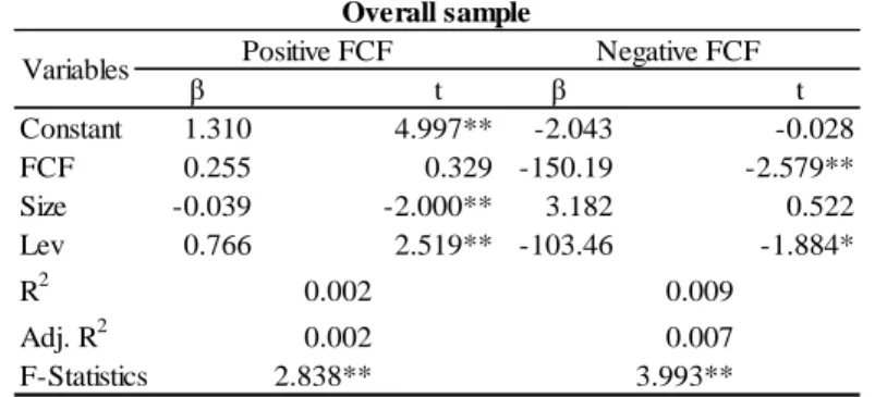
** and * means significance at 0.05 level and 0.1 level, respectively

β t β t Constant 1.310 4.997** -2.043 -0.028 FCF 0.255 0.329 -150.19 -2.579** Size -0.039 -2.000** 3.182 0.522 Lev 0.766 2.519** -103.46 -1.884* R2 0.002 0.009 Adj. R2 0.002 0.007 F-Statistics 2.838** 3.993** Overall sample

(29)

19

For other operating expenses, in these two subsamples, FCF is not significant.

Table IX – Other operating expenses and FCF - Positive FCF VS Negative FCF

In tables X and XI, only negative FCF subsamples have a significant relationship, showing no evidence of the FCF hypothesis for net operating income volatility and net income volatility.

Table X - Net Operating Income Volatility and FCF - Positive FCF VS Negative FCF

Table XI - Net Income Volatility and FCF - Positive FCF VS Negative FCF

To summarize, for the overall sample, in the negative FCF subsample analysis the results stay in the same line as the ones drawn before in sub-section 5.3.1.1., showing no evidence of Jensen’s FCF theory, revealing that when FCF does not exist, managers do not harm the company. Thus, if companies reduce FCF from managers’

β t β t Constant 0.628 3.531** -8.110 -0.130 FCF 0.512 0.974 -54.384 -1.092 Size -0.027 -2.031** 3.565 0.684 Lev 0.459 2.229** -83.364 -1.775* R2 0.002 0.004 Adj. R2 0.001 0.001 F-Statistics 2.709** 1.617

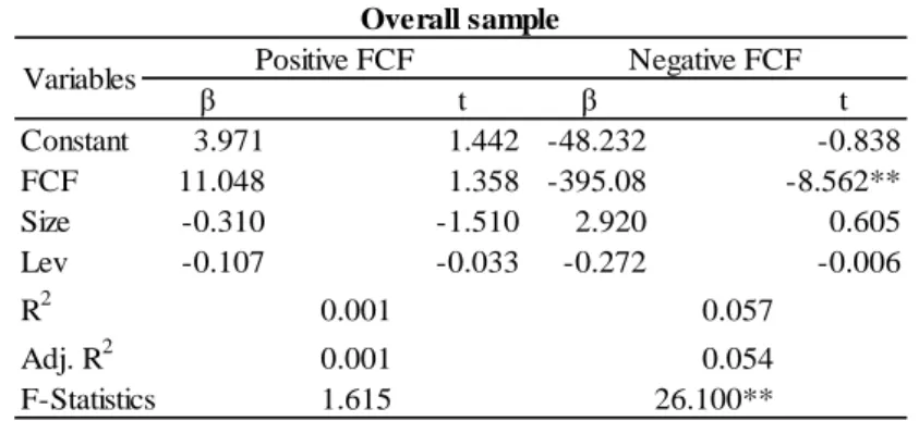
Overall sample β t β t Constant 3.971 1.442 -48.232 -0.838 FCF 11.048 1.358 -395.08 -8.562** Size -0.310 -1.510 2.920 0.605 Lev -0.107 -0.033 -0.272 -0.006 R2 0.001 0.057 Adj. R2 0.001 0.054 F-Statistics 1.615 26.100** Overall sample

β t β t Constant 3.687 1.483 -55.296 -0.980 FCF 11.134 1.516 -377.71 -8.353** Size -0.300 -1.619 3.746 0.792 Lev 0.903 0.313 -6.269 -0.147 R2 0.002 0.054 Adj. R2 0.001 0.054 F-Statistics 1.802 24.714** Overall sample

(30)

20

control it can diminish agency costs (Park & Jang, 2013). Methods such as leverage increase (Jensen, 1986; Gul & Tsui, 1998), pay-out cash flows to shareholders (La Porta, 2000) or share repurchase (Grullon & Michaely, 2004) are used to decrease FCF in a firm. Still, for the positive FCF subsample, the associations point to the increase of agency costs in the presence of FCF, however there is never a significant relationship.

Impact of crisis

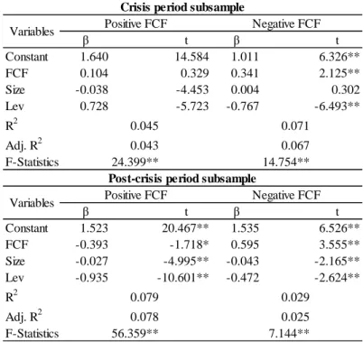
Analysing table XII, asset turnover and FCF relationship, during the crisis period subsample, is significant only in the negative FCF subsample, showing, as before, no evidence of the FCF hypothesis. In the post-crisis period subsample, we can see a non-linear relationship. In the positive FCF subsample the relationship is negative and in the negative FCF subsample the relationship is positive.

Table XII - Asset Turnover and FCF - Positive FCF VS Negative FCF and the impact of the crisis

In tables XIII and XIV, FCF is only significant for the crisis period subsample, in the negative FCF subsample, and it follows the same pattern, showing decreasing expenses as FCF increases, pointing to a cost-efficient management (Wang, 2010). Even though the associations are not significant, we can still conclude that there are non-linear relationships between positive FCF and negative FCF subsamples, for both the crisis period and post-crisis period subsamples.

β t β t Constant 1.640 14.584 1.011 6.326** FCF 0.104 0.329 0.341 2.125** Size -0.038 -4.453 0.004 0.302 Lev 0.728 -5.723 -0.767 -6.493** R2 0.045 0.071 Adj. R2 0.043 0.067 F-Statistics 24.399** 14.754** β t β t Constant 1.523 20.467** 1.535 6.526** FCF -0.393 -1.718* 0.595 3.555** Size -0.027 -4.995** -0.043 -2.165** Lev -0.935 -10.601** -0.472 -2.624** R2 0.079 0.029 Adj. R2 0.078 0.025 F-Statistics 56.359** 7.144**

Crisis period subsample

Post-crisis period subsample

** and * means significance at 0.05 level and 0.1 level, respectively Variables Positive FCF

Variables Positive FCF

Negative FCF

(31)

21

Table XIII - Operating expenses and FCF - Positive FCF VS Negative FCF and the impact of the crisis

Table XIV - Other operating expenses and FCF - Positive FCF VS Negative FCF and the impact of the crisis

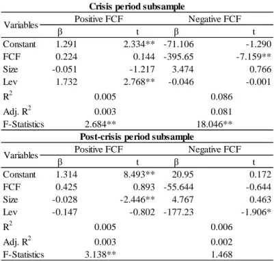
Analysing table XV and XVI, FCF has a significant relationship with net operating income volatility and net income volatility in negative FCF, for both subsamples, still not consistent with the FCF hypothesis.

β t β t Constant 1.291 2.334** -71.106 -1.290 FCF 0.224 0.144 -395.65 -7.159** Size -0.051 -1.217 3.474 0.766 Lev 1.732 2.768** -0.046 -0.001 R2 0.005 0.086 Adj. R2 0.003 0.081 F-Statistics 2.684** 18.046** β t β t Constant 1.314 8.493** 20.95 0.172 FCF 0.425 0.893 -55.644 -0.644 Size -0.028 -2.446** 4.767 0.463 Lev -0.147 -0.802 -177.23 -1.906* R2 0.005 0.006 Adj. R2 0.003 0.002 F-Statistics 3.138** 1.468

β t β t Constant 0.686 1.745* -16.270 -1.125 FCF 0.689 0.621 -105.87 -7.301** Size -0.040 -1.343 0.780 0.655 Lev 1.061 2.385** -1.455 -0.136 R2 0.004 0.090 Adj. R2 0.002 0.085 F-Statistics 2.141 19.033** β t β t Constant 0.567 14.072** -12.697 -0.116 FCF 0.408 3.300** -30.847 -0.395 Size -0.015 -4.989** 6.547 0.704 Lev -0.107 -2.243** -145.87 -1.738* R2 0.027 0.005 Adj. R2 0.025 0.001 F-Statistics 17.838** 1.131 ** and * means significance at 0.05 level and 0.1 level, respectively

(32)

22

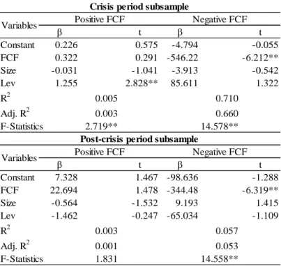
Table XV - Net Operating Income Volatility and FCF - Positive FCF VS Negative FCF and the impact of the crisis

Table XVI - Net Income Volatility and FCF - Positive FCF VS Negative FCF and the impact of the crisis β t β t Constant 0.226 0.575 -4.794 -0.055 FCF 0.322 0.291 -546.22 -6.212** Size -0.031 -1.041 -3.913 -0.542 Lev 1.255 2.828** 85.611 1.322 R2 0.005 0.710 Adj. R2 0.003 0.660 F-Statistics 2.719** 14.578** β t β t Constant 7.328 1.467 -98.636 -1.288 FCF 22.694 1.478 -344.48 -6.319** Size -0.564 -1.532 9.193 1.415 Lev -1.462 -0.247 -65.034 -1.109 R2 0.003 0.057 Adj. R2 0.001 0.053 F-Statistics 1.831 14.558**

β t β t Constant 0.132 0.176 -5.027 -0.062 FCF 1.722 0.815 -501.41 -6.175** Size -0.046 -0.802 -3.557 -0.533 Lev 2.707 3.195** 79.947 1.337 R2 0.007 0.070 Adj. R2 0.005 0.065 F-Statistics 3.431** 14.392** β t β t Constant 7.328 1.467 -108.688 -1.389 FCF 22.694 1.478 -336.61 -6.042** Size -0.564 -1.532 10.287 1.550 Lev -1.462 -0.247 -71.984 -1.202 R2 0.003 0.053 Adj. R2 0.001 0.049 F-Statistics 1.831 13.409** ** and * means significance at 0.05 level and 0.1 level, respectively

(33)

23

5.3.2. FCF and agency costs impact on operating performance 5.3.2.1 Overall Sample

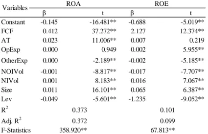
In table XVII we can see the relationship between operating performance, FCF and agency costs.

Table XVII - Operating performance, FCF and Agency Costs for the overall sample

The relationship between ROA and FCF is significant and positive, as concluded by Wang (2010) and Chung et al (2005). ROE presents the same results concerning FCF, indicating no evidence of the FCF hypothesis. This is in line with Gregory (2005), who states that firms with higher level of FCF perform better than its peers.

All agency costs’ variables present significant associations with ROA, except net operating income volatility and other operating expenses that agree with the agency theory, affecting negatively the firm’s performance and consistent with Khidmat & Rehman (2014). Regarding ROE, the agency costs’ variables in line with the agency theory are the same as in ROA.

Adding the impact of the crisis to the analysis above and dividing the sample into two sub periods, we can arrive to similar conclusions.

In the next table, we conclude that there are still no evidences of the FCF theory, since the relationship between ROA and FCF is significant and positive for both subsamples. The net operating income volatility, alongside with other operating expenses, remain the agency costs’ variables that affect negatively firm’s performance, following the agency theory.

β t β t Constant -0.145 -16.481** -0.688 -5.019** FCF 0.412 37.272** 2.127 12.374** AT 0.023 11.006** 0.007 0.219 OpExp 0.000 0.949 0.002 5.955** OtherExp 0.000 -2.189** -0.002 -5.185** NOIVol -0.001 -8.817** -0.017 -7.707** NIVol 0.001 8.183** 0.016 7.067** Size 0.011 16.101** 0.065 6.387** Lev -0.049 -5.601** -1.235 -9.052** R2 0.373 0.101 Adj. R2 0.372 0.099 F-Statistics 358.920** 67.813**

(34)

24

Table XVIII - ROA, FCF and Agency Costs - impact of the crisis

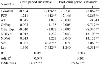
In table XIX, ROE relationship with FCF in both subsamples remains the same as in the overall sample analysed previously, without FCF hypothesis’ evidences. In the post-crisis period subsample operating expenses and net operating income volatility affect negatively firm’s performance, however in the crisis period subsample, even though these two variables remain with a negative relationship with ROE, none of the agency costs’ variables is significant.

Table XIX - ROE, FCF and Agency Costs - impact of the crisis

Therefore, if we add the impact of a financial crisis, the conclusions do not change much, regarding the firm’s operating performance. As studied by Garcia-Appendini & Montoriol-Garriga (2012), having a high level of cash can be an advantage during a financial crisis, as external financing becomes more expensive. Furthermore, they concluded that liquid firms show better performance levels during a period of crisis. β t β t Constant -0.112 -9.352** -0.162 -13.308** FCF 0.264 15.028** 0.458 32.627** AT 0.021 7.340** 0.023 7.898** OpExp 0.001 8.349** 0.000 4.986** OtherExp -0.006 -8.894** 0.000 -5.222** NOIVol -0.004 -6.065** -0.002 -11.431** NIVol 0.004 5.966** 0.002 10.863** Size 0.010 10.517** 0.011 12.553** Lev -0.090 -7.606** -0.090 -2.332** R2 0.306 0.451 Adj. R2 0.304 0.450 F-Statistics 118.028** 275.696**

β t β t Constant -0.584 -3.126** -0.731 -3.867** FCF 1.211 4.442** 2.146 9.865** AT 0.045 1.028 -0.038 -0.843 OpExp 0.003 1.138 0.005 9.717** OtherExp -0.010 -1.022 -0.005 -8.345** NOIVol -0.012 -1.232 -0.043 -15.100** NIVol 0.013 1.223 0.040 14.122** Size 0.061 4.287** 0.071 5.063** Lev -1.360 -7.422** -1.240 -6.511** R2 0.050 0.203 Adj. R2 0.047 0.201 F-Statistics 14.127** 85.672**

(35)

25

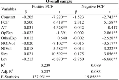
5.3.2.3 Robustness Checks Overall Sample

Now if we split the overall sample into positive and negative FCF subsamples, FCF maintains a significant relationship with ROA, only for the positive FCF subsample. Relative to agency costs, when there is positive FCF, operating expenses and net operating income volatility affect the company negatively. In the negative FCF subsample, only net operating income volatility follows the agency theory.

Table XX – ROA, FCF and Agency Costs- Positive FCF VS Negative FCF

Concerning ROE, we can see that FCF has a positive and significant relationship with ROE for both subsamples. Net operating income volatility is the only variable that follows agency theory in both subsamples, but when there is negative FCF, other operating expenses is also consistent with the theory.

Table XXI – ROE, FCF and Agency Costs - Positive FCF VS Negative FCF

β t β t Constant -0.048 -6.355** -0.326 -11.674** FCF 0.233 11.240** 0.340 15.063 AT 0.014 7.266** 0.035 6.924 OpExp -0.012 -2.883** 0.000 -0.011 OtherExp 0.011 1.882* 0.000 -0.733 NOIVol -0.004 -6.054** -0.001 -4.475** NIVol 0.004 5.331** 0.001 4.136** Size 0.006 12.217** 0.021 9.344** Lev -0.098 -11.878** 0.032 1.558 R2 0.201 0.347 Adj. R2 0.200 0.343 F-Statistics 110.981** 86.534** Overall sample

β t β t Constant -0.205 -7.220** -1.523 -2.743** FCF 0.500 6.418** 2.312 5.158** AT 0.031 4.328** -0.042 -0.417 OpExp -0.022 -1.391 0.002 2.861** OtherExp 0.012 0.540 -0.002 -2.528** NOIVol -0.020 -7.102** -0.015 -3.517** NIVol 0.018 5.582** 0.014 3.222** Size 0.021 10.592** 0.175 3.856** Lev -0.213 -6.870** -2.750 -6.666** R2 0.239 0.089 Adj. R2 0.237 0.083 F-Statistics 137.931** 15.858** Overall sample

(36)

26

Thus, from this analysis we can say that FCF remains a positive influence on firm’s performance, whether it is positive or negative. Wang (2010) defends that the presence of FCF increases firm’s performance. One of the reasons that can justify these results, namely the lack of evidence of the managers’ abuse of FCF is presented by Brush et al (2000), who states that owner-managed companies with FCF are the ones showing the highest levels of performance.

Impact of the crisis

In table XXII, FCF remains a significant variable and keeps a positive association with ROA and, generally, the agency costs’ variables that follow the agency theory are also operating expenses, other operating expenses and net operating income volatility.

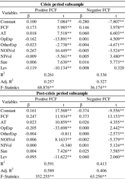
Table XXII – ROA, FCF and Agency Costs- Positive FCF VS Negative FCF and the impact of the crisis

β t β t Constant 0.100 7.084** -0.280 -7.807** FCF 0.173 5.985** 0.146 3.978** AT 0.018 7.518** 0.060 6.603** OpExp -0.162 -13.891** 0.001 4.509** OtherExp -0.023 -2.738** -0.004 -4.671** NOIVol 0.267 16.449** -0.005 -3.524** NIVol -0.009 -5.561** 0.005 3.480** Size 0.006 7.630** 0.016 5.773** Lev -0.119 -10.134** 0.008 0.320 R2 0.261 0.336 Adj. R2 0.257 0.327 F-Statistics 68.876** 36.174** β t β t Constant 0.161 17.568** -0.374 -9.556** FCF 0.247 11.934** 0.373 13.153** AT 0.023 10.859** 0.026 4.355** OpExp -0.205 -33.698** 0.000 2.442** OtherExp -0.004 -0.811 0.000 -2.573** NOIVol 0.006 8.1633** -0.002 -5.379** NIVol 0.000 -0.340 0.001 5.124** Size 0.004 7.426** 0.025 7.585** Lev -0.095 -11.622** 0.060 2.060** R2 0.591 0.413 Adj. R2 0.589 0.406 F-Statistics 352.255** 63.256**

(37)

27

In table XXIII, ROE and FCF have a positive relationship and, like ROA, operating expenses, other operating expenses and net operating income volatility are consistent with the agency theory.

Table XXIII – ROE, FCF and Agency Costs- Positive FCF VS Negative FCF and the impact of the crisis

In both tables, XXII and XXIII, for operating expenses and net operating income volatility we can find non-linear relationships in both subsamples, the crisis period and the post-crisis period.

5.3.3. FCF and agency costs impact on firm value 5.3.3.1 Overall Sample

As studied by Lang et al (1991), and according to the FCF hypothesis, firms with higher FCF levels will have a lower q ratio, making investments that harm shareholders. β t β t Constant 0.065 1.118 -1.028 -1.315 FCF 0.479 4.027** 1.211 1.511 AT 0.039 3.892** 0.065 0.331 OpExp -0.323 -6.708** 0.003 0.514 OtherExp -0.077 -2.229** -0.009 -0.440 NOIVol 0.539 8.045** -0.015 -0.0513 NIVol -0.005 -0.788 0.017 0.512 Size 0.022 6.895** 0.127 2.057** Lev -0.268 -5.545** -2.888 -5.015** R2 0.113 0.052 Adj. R2 0.108 0.039 F-Statistics 24.694** 3.938** β t β t Constant 0.309 7.661** -2.152 -2.854** FCF 0.422 4.627** 1.888 3.454** AT 0.053 5.617** -0.082 -0.712 OpExp -0.472 -17.543** 0.005 5.200** OtherExp -0.014 -0.564 -0.005 -4.495** NOIVol 0.006 2.045** -0.044 -7.745** NIVol 0.004 1.176 0.041 7.276** Size 0.013 5.773** 0.219 3.506** Lev -0.200 -5.557** -2.536 -4.495** R2 0.482 0.187 Adj. R2 0.480 0.178 F-Statistics 227.121** 20.761**

(38)

28

In table XXIV, the relationship between Tobin’s Q and FCF is negative and significant, consistent with Heydari et al (2014), that concluded that an increase in FCF does not show the management’s ability in rising firm value, confirming the FCF theory. From the variables of agency costs, asset turnover, operating expenses ratio and net income volatility are the ones that generally predict the agency theory (Khidmat & Rehman, 2014).

Table XXIV - Firm Value, FCF and Agency Costs for the overall sample

Comparing the variables in the crisis period subsample and the post-crisis period subsample, we arrive at different conclusions regarding the FCF hypothesis.

Table XXV - Tobin's Q, FCF and Agency Costs relationship - impact of the crisis

β t Constant 1.719 17.298** FCF -0.656 -5.294** AT -0.128 -5.480** OpExp -0.002 -6.655** OtherExp 0.002 6.265** NOIVol 0.021 13.284** NIVol -0.020 -12.338** Size -0.019 -2.549** Lev -1.144 -11.634** Rm -0.032 -0.196 R2 0.111 Adj. R2 0.110 F-Statistics 67.172** Variables Tobin's Q

β t β t Constant 1.230 10.054** 1.945 13.861** FCF 0.359 2.017** -0.958 -6.003** AT -0.066 -2.343** -0.128 -3.897** OpExp -0.044 -24.661** -0.001 -3.149** OtherExp 0.161 24.419** 0.001 3.446** NOIVol 0.044 6.692** 0.019 9.184** NIVol -0.045 -6.342** -0.018 -8.944** Size -0.011 -1.154 -0.023 -2.268** Lev -0.666 -5.571** -1.367 -9.798** Rm 0.107 0.715 -0.036 -0.095 R2 0.330 0.098 Adj. R2 0.327 0.095 F-Statistics 117.106** 32.512**