Modelling the interaction effects of the high-speed train-track-bridge system using ADINA

(1)

MODELLING THE INTERACTION EFFECTS OF THE HIGH-SPEED

TRAIN–TRACK–BRIDGE SYSTEM USING ADINA

Constança Rigueiro

Department of Civil Engineering, Polytechnic Institute of Castelo Branco Portugal

Carlos Rebelo, Luis Simões da Silva

Department of Civil Engineering, University of Coimbra Portugal

Email: crebelo@dec.uc.pt

ABSTRACT

The main purpose of this paper is to present some results concerning the investigation of the effects of the vehicle-bridge interaction in simply supported medium span viaducts, including the modelling of the ballast-rail track system. This system is modelled using the rail stiffness in vertical and longitudinal directions, including the rail pad and the sleepers, and the ballast as a system of vertical springs, dampers and masses. A simplified vehicle model proposed by the European Railway Research Institute (ERRI D214, 1999), taking into account the vehicle primary suspension characteristics and the mass of the bogie is used with the contact algorithm implemented in the software ADINA to evaluate the response acceleration of a simply supported medium span concrete viaduct. The results are compared with those from the moving loads model for a wide range of train speeds.

INTRODUCTION

Due to the increasing interest in the high speed railway transportation, the research on the vibration of bridges under moving vehicles has been growing much then ever. The investigation started to be analytical, with approximate solutions for some simple but fundamental problems (for example, Fryba, 1999, Biggs, 1964). Nowadays, the investigation use more realistic and complex bridge and vehicle models to analyse the bridge vibrations (Yang et al, 2004, Xia 2003). However, in these works, the effects of the ballasted tracks were only partially accounted for, or they have been completely neglected.

The most frequently used model for the dynamic calculations of the train is the moving loads model. This model does not take into account the inertial effects of the train masses and the stiffness and damping of the primary suspension of the vehicle. As a consequence, the train is modelled as a series of point loads with constant values travelling over the bridge at a constant speed.

The committee D214 of the European Research Institute (ERRI) reports that, for short span bridges, the vertical accelerations of the deck predicted by the moving loads model reach unrealistic values, which are much higher than the limit of 3,5 m/s2 imposed for the bridges with ballasted track by the Criteria for Traffic Safety (EN1990-prAnnex A2, 2002). This committee also pointed out that, for the resonance speeds, the predicted bridge response when using train/bridge interaction is significantly lower than the response acceleration obtained with the moving loads model.

This ongoing research aims to highlight and evaluate those differences concerning the models results. Therefore, the main purpose of this paper is to analyse the influence of train/bridge

(2)

interaction in simply supported medium span viaducts, including the modelling of the ballasted rail track system on the bridge. Comparisons of the numerical simulations results are carried out for a real bridge, using the contact algorithm implemented in the software ADINA. To obtain the vehicle/bridge interaction effects, the vehicle is usually modelled as a two-degree-of-freedom dynamic unit (see Figure 6), or as a rigid beam supported on two-spring-damper systems to take into account the pitching effect of the vehicle (Yang, 2004). In this research only the first simplified model is considered to analyse the influence on the bridge response displacements and accelerations.

The inclusion of the ballasted rail track system in the numerical model allows of taking into account the longitudinal distribution of the loads through the sleepers and ballast layer. Several models (Figures 1 to 3) are considered for the evaluation. In general, they include vertical springs, dampers and masses, which are interposed between the vehicle and the structure. Although both the dynamic response of the track and the bridge response was computed, only the response of the bridge is presented here.

DYNAMIC MODELS OF THE RAILWAY BALLASTED TRACK

The railway ballasted track model is made of several elements which represent the rails, the sleepers, the connections between rails and sleepers, and the ballast. The rails are an important component in the track structure, since they transfer the wheel loads and distribute them over the sleepers and supports, guide the wheels in the lateral direction, provide a smooth running surface and distribute acceleration and braking forces over the supports. In Europe the typical rail used in the high speeds lines is the flat-bottom rail, UIC60.

The connections rail/sleeper are materialized by fastenings and rail pads. This system provides the transfer of the rail forces to the sleepers, damps the vibrations and impacts caused by the moving traffic and retains the track gauge and rail inclination within certain tolerances.

The sleepers are elements positioned just below the rails usually made of timber or concrete. They provide support for the rail, sustain rail forces and transfer them as uniformly as possible to the ballast. They preserve track gauge and rail inclination and provide adequate electrical insulation between both rails. The sleepers must be resistant against mechanical and weathering influences over a long period.

Finally, the ballast bed consists of a layer of a coarse-sized, non cohesive, granular material. Traditionally angular, crushed, hard stones and rocks have been considered good ballast materials. The interlocking of ballast grains and their confined condition inside the ballast bed permit the load distributing function and the damping. They also provide the lateral and longitudinal support of the track, as well as the draining effect. The thickness of the ballast bed should allow the sub grade to be loaded as uniformly as possible. The usual depth for the ballast is about 0.3 meters measured from the underside of the sleeper.

In the early studies, the models of the ballasted track were developed in order to investigate the train/track interaction problem. A review of these studies is presented in Fryba, 1999. In the 1900’s Timoshenko published papers on the strength of rails; later on, Inglis, was active in this issue. Knothe, 1993, and Popp, 1999, presented an overview of existing tracks models in the field of train/track interaction. The main purpose of these studies was to evaluate the deflections of the track and the vertical displacements of the vehicles, while the contact force

(3)

wheel/rail is evaluated in the calculations. Complete models of the vehicles and the effects of the wheel and rail irregularities were also investigated.

A large variety of ballasted track models has been investigated, from simple 2D model, where a single rail is modeled as an infinite Bernoulli-Euler or Timoshenko beam resting on supports defined by springs, dampers and point masses, to more complex 3D models, where both rails are taken into account and bending and shear deformation of the sleepers are included. In these models, the ballast bed is included through vertical spring and damper elements. Some of these models consider the mass of the ballast as a point mass located below each sleeper and its value is taken relative to the amount of stiffness and damping. Furthermore, shear springs and dampers may interconnect these masses (Zhai, 2003).

The values for the mechanical properties of the track components, such as mass, inertia and elasticity, are mentioned as an essential input for dynamic track behavior and, of course, for the study of the interaction between train and track.

Since the focus of the present work is on the influence of the ballast track on the vertical vibrations of the railway bridges obtained by comparison of the numerical results with the dynamic response obtained from field measurements, only the 2D tracks models were considered, neglecting unimportant torsion effects.

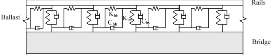
For this purpose, three different models of ballasted tracks are presented in Figures 1, 2 and 3 (Man, 2002), (Yang, 2004), (ERRI, 1999). In Model I the rails are considered as infinite long beams with in-plane and out-of-plane flexural stiffness as well as axial stiffness. The linear springs and dampers on the vertical and longitudinal directions represent the ballast. These three models are included in the finite element model of the bridge, which is acted by moving loads representing real trains. The model parameters remain constant along the track, despite some deviations due to construction and maintenance works. In the other two models, Model II and Model III, the connections between rail and sleeper are included as linear springs and viscous dampers acting in parallel. Their elastic and damping properties are mainly determined by the properties of the material and the manufacturing processes. The sleepers are included as rigid bodies with point mass. The ballast bed is included as discrete linear springs and viscous dampers. In Model III the mass of the ballast is included as point mass instead of distributed mass, and springs and dampers are used to simulate the connection between bridge and ballast (ERRI, 1999). The parameters used in Model II were obtained from (Man, 2002).

The values of the mechanical properties for each model are included in Table 1 to Table 3.

(4)

Figure 2: Ballasted track Model II (Man, 2002). Cbs Kbs Kbb Cbb Rails Sleeper Railpads Ballast Krp Crp Ms Bridge Mb

Figure 3: Ballasted track Model III (ERRI, 1999).

Components of the track model I Notation Value Units

Rail UIC60

Young Modulus Er 210E+09 N/m

2

Density

ρ

r 7850 kg/m

3

Flexural moment of inertia Ir 3055E-08 m

4

Sectional area Ar 76.9E-04 m

2 Ballast

Per unit of length Vertical stiffness Kbv 104E+06 N/m

Per unit of length Vertical damping Cbv 50E+03 N.s/m

Per unit of length Horizontal stiffness Kbh 104E+06 N/m

Per unit of length Horizontal damping Cbh 50E+03 N.s/m

(5)

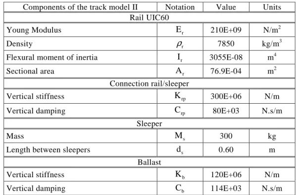
Components of the track model II Notation Value Units Rail UIC60

2

Density

ρ

r 7850 kg/m

3

4

2 Connection rail/sleeper

Vertical stiffness Krp 300E+06 N/m

Vertical damping Crp 80E+03 N.s/m

Sleeper

Mass Ms 300 kg

Length between sleepers ds 0.60 m

Ballast

Vertical stiffness Kb 120E+06 N/m

Vertical damping Cb 114E+03 N.s/m

Table 2: Properties of track Model II (Man, 2002).

Components of the track model III Notation Value Units

Rail UIC60

2

Density

ρ

r 7850 kg/m

3

4

2 Connection rail/sleeper

Vertical stiffness Krp 500E+06 N/m

Vertical damping Crp 200E+03 N.s/m

Sleeper

Mass Ms 290 kg

Length between sleepers ds 0.60 m

Ballast

Vertical stiffness ballast/sleeper Kbs 538E+06 N/m

Vertical damping ballast/sleeper Cbs 120E+03 N.s/m

Mass Mb 412 kg

Vertical stiffness bridge/ballast Kbb 1000E+06 N/m

Vertical damping bridge/ballast Cbb 50E+03 N.s/m

(6)

THE INTERACTION MODELLING USING ADINA

In the present study, only plane models are considered. The vertical displacements of the railway vehicles are analyzed and the two rails are effectively treated as a single one in the subsequent analysis. Figure 4 shows a typical vehicle element with a 2-DOF acting on the bridge/track system. The upper and lower beam elements modeling the rail and the bridge deck respectively are interconnected by the rail track model as mention before. Since the high speed train ICE2 is considered for the analysis, it must be assumed that there are 56 moving vehicles in direct contact with the bridge or with the platform that must be modeled before and after the bridge itself.

Figure 4: Vehicle/track/bridge interaction model.

Same Considerations About the Contact Algorithm

The contact algorithms in ADINA are described in its manual and in other references (Bathe, 1985; Bathe, 1996). This algorithm is presented as a solution procedure for the analysis of planar or axisymmetric contact problems involving sticking, frictional, sliding and separation where large deformation is present. The contact conditions are imposed using the total potential of the contact forces with the geometric compatibility conditions along the contact surfaces, which leads to surface tractions from the externally applied forces. Same key aspects of the procedure are the contact matrices, the use of distributed tractions on the contact segments for deciding whether a node is sticking or releasing and the evaluation of the nodal point contact forces. The number of equations due to the contact conditions is dynamically adjusted to solve two equations for each node in contact, if the node is in sticking condition, and one equation, if the node is in sliding condition, which is the case for the present study.

(7)

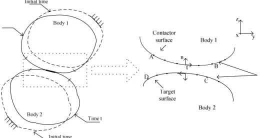
Figure 5 shows schematically the contact problem. Although in this figure only two bodies are represented, the algorithm can be applied to situations wehere more bodies are in contact. The figure shows two generic bodies which come into contact along the contact surfaces, the contactor surface from A to B, and the target surface from C to D, in the time t . Due to this contact, forces are developed acting along the region of contact, the contact segment. These forces are equal and opposite and can be transformed into normal and tangential vectors. The normal tractions can only exert compressive action, and tangential tractions satisfy a law of frictional resistance, if it exists.

Besides the elastic forces considered in the static analysis, the dynamic analysis of the contact forces includes the inertia and the cinematic force effects of each body, whose interfaces conditions must be satisfied at all instances of time, requiring displacement, velocity, and acceleration compatibility between the contacting segments. The software ADINA has explicit and implicit methods for the computations at each time step. In the present case we have applied an implicit method of time integration of the equilibrium equations, as we will discuss later on.

For the high speed train ICE2 model, a contact surface for each vehicle is needed in addition to the contact surface for the bridge/rail. This means a total number of 57 contact surfaces and 56 contact pairs.

The Vehicle Model

A sprung mass model, denoted in the bibliography as a simplified vehicle model, defines the vehicle model. The sprung mass model is conceived as a two-node system, with each node associated with lumped masses. The stiffness and damping of the suspension, denoted by C _v andk , respectively, correspond to the primary suspension of the train vehicle. The mass of _v the wheel is M and the lumped mass from the car body is _w M (equal to a quarter of the _v mass of the car body and bogie mass). The 56 vehicles travel at a constant speedv . _i

Figure 6: Sprung mass model used in ADINA.

The vertical displacements of the masses M and _w M are _v z and ₁ z , respectively, and they ₂ are defined as being vertical and measured from the static equilibrium positions. Let F be the _ci contact force between the ith vehicle and the rail. It can be express in terms of static force

wi

F , the total weight of the two masses, Fwi =

(

Mv+Mw

)

⋅g, with g denoting the acceleration of gravity, and the variation of contact forces ∆F_ci corresponding to the interaction or time dependent variation of the contact force:

(8)

ci wi ci

F =F + ∆F (1)

The equations of motions for the sprung mass model shown in Figure 6 can be written as follows (Biggs, 1964): w 1 v v 1 v v 1 c v 2 v v 2 v v 2 M 0 z C C z K K z F 0 M z C C z K K z 0 − −            + + =           ₋  ₋                ɺɺ ɺ ɺɺ ɺ (2)

The contact force must be positive,F_c≥0, to exclude the possibility of lost contact between the wheels and the rail.

Solution of the Equilibrium Equations

There are several methods available for the time integration in software ADINA. The explicit time integration method implemented corresponds to the central difference scheme. The main advantage of this method is the mass matrix is diagonal and the solution of the displacements at time t+ ∆t does not involve a triangular factorization of the stiffness matrix in the step by step solution. However, the central difference method is a scheme only conditionally stable, which means that it requires the use of a time step t∆ smaller than a critical time step ∆t_cr. If a time step larger than ∆t_cr is used, the integration becomes unstable and the errors in the computation grow and make the calculations worthless in most cases. Consequently, the use of this scheme is limited to certain problems.

The implicit methods of the Newmark family methods, the Wilson-θ method and the Composite method, which includes a third parameter

α

for the resolution of the equilibrium equations, are available in ADINA. The Composite method is a time integration scheme for nonlinear analysis, where the displacements, velocities and accelerations are solved for a time t+ ∆α t, where

α

∈

[ ]

0,1 . Whenα =0.5, it is the same as the Newmark method. Since these implicit methods are unconditionally stable, the step ∆t can be selected independent of stability considerations and thus they can result in a substantially saving of computational effort. However, these schemes require the triangularization of the stiffness matrix.

According to EN1990-prAnnex A2, 2002, for the determination of the maximum deck acceleration, the frequencies in the dynamic analysis should be considered up to a maximum of: i) 30 Hz ; ii)1.5 times the frequency of the first mode shape of the structural element being considered, including at least the first three modes shapes. For that reason, in addition to being unconditionally stable, when only low mode response is of interest it is desirable that the integration scheme has the ability to damp out the spurious participation of the higher modes through numerical dissipation. The Wilson θ method and the Newmark family of methods, restricted to parameter values of

γ

>1 2 and β ≥0.25× +

(

γ 1 2

)

2, where the amount of dissipation, for a fixed time step t∆ , is increased by increasing γ , possess this advantage. On the other hand, the dissipative properties of this family of algorithms are considered less efficient then those of the Wilson θ method, since the lower modes are strongly affected. The Wilson θ method, with θ =1.4, is highly dissipative at the highest modes, unconditionally stable and accurate when ∆t T_n ≤0.01, where T is the lowest _n vibration period to take into account in the structural response analysis, (Bathe, 1996).

(9)

Considering all the pros and contras of the methods, the dynamic response of the bridge was obtained by using the Wilson θ method.

A NUMERICAL EXAMPLE

Bridge Model

In order to investigate the influence of the interaction in the dynamic behavior, a simply supported bridge was considered, with a span length of 23.5 m , 0.4835 m4of cross sectional moment of inertia and 21080 kg m of mass per unit length along the axis. The Young modulus was taken equal to 40 GPa . This leads to a fundamental frequency near to 2.70 Hz , a static deflection at mid span due to the ‘Load Model 71’ equal to δ =23.04mm and a

L

δ

_≃1020. The ‘Load Model 71’ is a static load pattern proposed by the Eurocode 1 (EN1991-2, 2003), for the design of railway bridges.

Concerning the damping, the Rayleigh matrix was used, that is, C= ⋅ + ⋅α M β K, with constants α =0.235 and β =3.640E 04− , which correspond to a damping ratio, for the first frequency of the bridge of about 1% . This is the value that is recommended by the Eurocode 1 for prestressed concrete railway bridges with span greater than 20 m .

Train Speeds

According to Eurocode 1, a series of train speeds up to the maximum design speed must be considered. The maximum design speed is 1.2 max imum× live speed at the site. Calculations were made for a series from 140 km / h up to maximum design speed of 300 km / h . The speed step used for these calculations was 5 km / h , smaller speed step was adopted with the purpose to match with the resonant speeds.

The High-speed Train ICE2

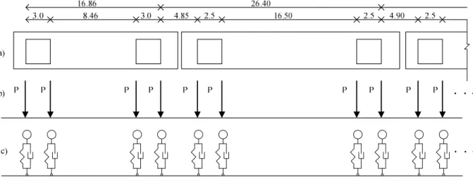
The high-speed train ICE2 consists of a total of 14 carriages including two power cars located in the front and in the rear of the train. It is a conventional train, that is, it possesses two bogies for each carriage. The Figure 7 represents part of the ICE2 train, in plan view, in the moving force model and in the moving vehicle model used for the interaction computations. Each bogie has two axles represented by two forces; the weigh of each axle is 195 kN for the power cars, and 112 kN for the intermediate carriages.

(10)

The passage of successive loadings with uniform spacing, in this case is 26.40 m , can excite the structure and create resonance. This effect can be pointed out in terms of a critical speed. In the present case the resonance speed can be calculated using the following formula

k cri. 0 D v n , i 1, 2, 3,..., n i = × = (3)

For i=1, D_k =26.40 m and n₀ =2.70 Hz the critical speed occur for ≈257 km / h. If i>1 is considered, the critical speeds will be inferior to the studied speed range.

The Moving Loads Model

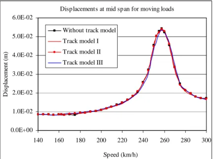
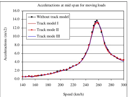
Considering the moving load model rolling on in the range of speeds mentioned above, for the several models of bridge, with and without the track ballast model, maximum values of the displacements and accelerations were computed. As we can see in Figure 8 and Figure 9, the responses of the bridge, for the maximum values of displacements and accelerations are very similar. Considering these results, it can be concluded that the presence of the railway track model does not influence the maximum response of the bridge for the moving load model. However, the use of the ballast track model suppresses the contribution of frequency components of the bridge response acting as a low pass filter. This effect can be shown in Figure 10, for a lower speed, 140 km / h , where the representation of the accelerations at the mid span of the bridge is made in the frequency domain. The contribution of the frequencies in the range 10-30 Hz are suppressed when the track model is included. From this point of view all the track models have the same behavior in filtering the higher frequencies.

Displacements at mid span for moving loads

0.0E+00 1.0E-02 2.0E-02 3.0E-02 4.0E-02 5.0E-02 6.0E-02 140 160 180 200 220 240 260 280 300 Speed (km/h) D is p la ce m en t (m )

Without track model Track model I Track model II Track model III

Figure 8: Maximum displacements at mid span considering the moving force model.

The Figure 10 also allows the conclusion that the application of the Wilson θ integration method leads to a good result in damping out the spurious participation of the higher modes, that is, the contribution of the frequencies higher than 30 Hz is very low as it is recommended by the EN1990-prAnnex A2.

(11)

Acceleractions at mid span for moving loads 0.0 2.0 4.0 6.0 8.0 10.0 12.0 14.0 16.0 140 160 180 200 220 240 260 280 300 Speed (km/h) A cc el er ac ti o n s (m /s 2 )

Without track model Track model I Track mode II Track mode III

Figure 9: Maximum accelerations at mid span considering the moving force model.

0.00E+00 2.00E-02 4.00E-02 6.00E-02 8.00E-02 1.00E-01 1.20E-01 1.40E-01 1.60E-01 0.0 10.0 20.0 30.0 40.0 50.0 60.0 70.0 80.0 90.0 100. 0 Frequency (Hz) A m p li tu d e

Without track model Track model I

Figure 10: Comparison of the accelerations of the bridge with a track model I and without track model in frequency domain during the passage of the ICE2 train at a speed of 140km/h, for the moving load model.

The Interaction Model

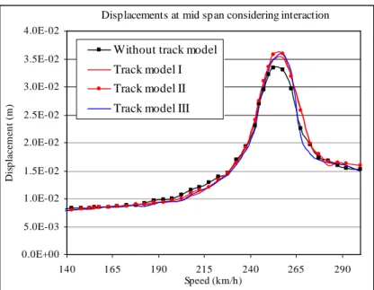
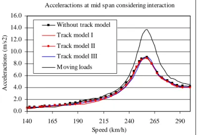
Considering now the results obtained when the vehicle/bridge or vehicle/track/bridge interaction is present, the maximum values of the displacement and acceleration response are represented in Figure 11 and Figure 12, respectively.

The resonance speed is reached at about the same value as before, but the maximum values of displacement and acceleration obtained with these models are much lower than those obtained with the moving loads model. The maximum displacement is 3.60 cm , obtained for the vehicle/track/bridge interaction models II and III. The maximum displacement obtained with the model without ballast track is 3,4 cm.

Considering the response accelerations, all the models furnish identical results. Out of the resonance situation the vehicle/bridge model, without track, shows modest higher values than the other models.

(12)

Displacements at mid span considering interaction 0.0E+00 5.0E-03 1.0E-02 1.5E-02 2.0E-02 2.5E-02 3.0E-02 3.5E-02 4.0E-02 140 165 190 215 240 265 290 Speed (km/h) D is p la c e m e n t (m )

Figure 11: Maximum displacements at mid span considering the interaction model.

Acceleractions at mid span considering interaction

0.0 1.0 2.0 3.0 4.0 5.0 6.0 7.0 8.0 9.0 10.0 140 165 190 215 240 265 290 Speed (km/h) A cc el er ac ti o n s (m /s 2 )

Figure 12: Maximum accelerations at mid span considering the interaction model.

Analyzing the comparison (see Figure 13) of the frequency response accelerations at the mid-span of the bridge taking into account the vehicle/track/bridge interaction model, with different systems and the vehicle/bridge interaction model, it can be concluded that the ballast track model acts like a low-pas filter. The results considering vehicle/bridge interaction, without any track model, show a contribution of the higher frequencies when compared with the equivalent system when the moving force model is used (compare Figures 10 and 13). The differences among the results of the several vehicle/track/bridge interaction models are small. Therefore, in Figure 13, only the results of the effects of the track ballast model III are represented, since this model seems to be the most efficient in damping the higher frequencies.

Figure 14 and Figure 15 compare the results obtained with the two different loading methodologies, the moving load model methodology and interaction model methodology. The

(13)

maximum values obtained with the interaction model are about 33% lower than the equivalent results obtained with the moving forces model.

0.0E+00 2.0E-02 4.0E-02 6.0E-02 8.0E-02 1.0E-01 1.2E-01 1.4E-01 1.6E-01 1.8E-01 0.0 10.0 20.0 30.0 40.0 50.0 60.0 70.0 80.0 90.0 100. 0 Frequency (Hz) A m p li tu d e

Without track model Track model III

Figure 13: Comparison of the accelerations of the bridge with a track model III and without track model in frequency domain during the passage of the ICE2 train at a speed of 140km/h, for the interaction model.

Displacement s at mid span considering interaction

0.0E+00 1.0E-02 2.0E-02 3.0E-02 4.0E-02 5.0E-02 6.0E-02 140 165 190 215 240 265 290 Speed (km/h) D is p la c e m e n t (m )

Without track model Track model I Track model II Track model III Moving loads

Figure 14: Comparison of the maximum displacements of the bridge for the interaction and moving loads models

Acceleractions at mid sp an considering interaction

0.0 2.0 4.0 6.0 8.0 10.0 12.0 14.0 16.0 140 165 190 215 240 265 290 Sp eed (km/h) A cc el er ac ti o n s (m /s 2 )

Without track model Track model I Track model II Track model III M oving loads

(14)

CONCLUSIONS

The main purpose of this investigation was the study of the behavior of simply supported railway bridges with medium span and low stiffness, subject to the high speed train ICE2, using two different methodologies for the loading models: the vehicle/track/bridge interaction methodology and the moving loads methodology. Additionally, three types of track models were considered

According to the results obtained for the acceleration in the frequency domain, it can be concluded that the use of the Wilson-θ method in railway problems shows to be suitable in filtering the high frequency components. The results reveal a good numerical dissipation of the spurious participation of the higher modes.

The response of the system track/bridge when subject to the moving loads model shows that the different track models do not influence the maximum displacements and accelerations. The results obtained for the response accelerations in the frequency domain show that those models act as a filter in the high frequency components.

Comparing the results obtained for the maximum displacements and accelerations at the mid span for the two different methodologies, interaction model and moving load model, it can be concluded that the use of the interaction model results in 33% lower displacements and accelerations. Therefore, the inclusion of the inertia effects of the moving vehicles contributes decisively to the reduction of the peak response.

REFERENCES

Biggs J.M. Introduction to structural dynamics. McGraw-Hill. London, 1964.

ERRI D214, Rail Bridges for speeds >200km/h. Final Report. European Rail Research Institute, 1999. Fryba L. Vibrations of solids and structures under moving loads. Thomas Telford, 1999.

Yang Y.B., Yau J.D., Wu Y.S. Bridge interactions dynamics with applications to high-speed railways. World Scientific, 2004.

Xia H., Zhang N., Roeck G. Dynamic analysis of high speed railway bridge under articulated trains. Computers and Structures 81, 2003, p. 2467-2478.

EN1991-2, Actions on structures – Part 2: General actions – Traffic loads on Bridges. European Committee for Standardization, CEN, 2003.

EN1990-prAnnex A2, Basis of Structural Design – Annex A2: Application for bridges (normative), Final Draft. European Committee for Standardization, CEN, 2002.

Bathe K J. Finite Element Procedures, prentice-Hall, 1996.

Bathe K.J., Chaudhary A., A Solution method for planar and axisymmetric contact problems, International Journal for Numerical Methods in Engineering, vol. 21, 61-88, 1985.

Zhai M, Wang Y, Lin H. Modelling and experiment of railway ballast vibrations, Journal of Sound and Vibration, 270, pp. 673-683, 2003.

Man A. A survey of dynamic railway track properties and their quality, PhD. Thesis, TU Delft, DUP – Science, Delft, 2002.