Massivel y parallel declarative computational models

(1)

MASSIVELY PARALLEL DECLARATIVE

COMPUTATIONAL MODELS

Rui Mário da Silva Machado

Tese apresentada à Universidade de Évora para obtenção do Grau de Doutor em Informática

ORIENTADOR: Salvador Pinto Abreu

ÉVORA, Julho de 2013

(2)

(3)

UNIVERSIDADE DE ´

EVORA

Massively Parallel Declarative

Computational Models

Rui M´

ario da Silva Machado

Tese apresentada à Universidade de Évora para obten¸cão

do grau de Doutor em Inform´atica

Orientador: Salvador Pinto Abreu

´

(4)

(5)

(6)

(7)

Acknowledgments

It is interesting to look back, remembering the circumstances and persons that crossed our path. When I started my PhD, I had no clue where it would take me. Now, looking back, it is my sincere conviction that it is the people that either leave a mark on you in some way or are present, sharing the roller coaster of the journey, what counts the most. Here I would like to thank them all, humbly apologising those I might overlook.

The first person I must thank to is Werner Kriechbaum. Werner was the person who shed the light to an option which I never considered before I met him. I will always be thankful for his mentor-ship, support and friendship.

I would like to thank to Salvador Abreu, my adviser. First of all, for his patience and readiness of advice when things were not looking so bright to me. But also for his guidance and discussions that shaped this work and allowed me to actually finish it.

My journey took place at the Fraunhofer ITWM. There I made friends, got introduced to the HPC community and learned a lot thanks to the great professionals of the HPC department. I would like to thank Franz-Josef Pfreundt for giving me the opportunity to join the department and making me feel welcome. To my office mate, Carsten Lojewski, who has become a good friend, from whom I learned a great deal of things and spent amazing moments. To all other colleagues and friends Mirko, Martin, Matthias, Ely, Jens, Valentin, Daniel for the interesting discussions, support and great Wednesday nights. To those outside my working place but who also contributed for the realisation of this work. I would like to thank Vasco Pedro for sharing PaCCS and his knowledge with me which allowed me to progress quickly. And to Daniel Diaz and Philip Codognet for the discussions, ideas and help that made this work a better one.

Finally, simple words for those without whom life would be meaningless and insignificant.

To all my friends for remembering that there is more to life than just work. To my

parents whose hard work and support allowed me to get a good education; for simply being present, always, whenever I needed them, for the good or for the bad. And my bro, who is a constant presence and source of strength and inspiration in my mind. Finally to my treasure, Tania, the person who felt more closely my moments of enthusiasm but also those of frustration. Her love and support, allowed me to relax on hard moments and to focus and avoid distractions when I needed to. I dedicate this work to you.

(8)

(9)

Abstract

Current computer archictectures are parallel, with an increasing number of processors. Parallel programming is an error-prone task and declarative models such as those based on constraints relieve the programmer from some of its difficult aspects, because they abstract control away.

In this work we study and develop techniques for declarative computational models based on constraints using GPI, aiming at large scale parallel execution.

The main contributions of this work are:

• A GPI implementation of a scalable dynamic load balancing scheme based on work stealing, suitable for tree shaped computations and effective for systems with thou-sands of threads.

• A parallel constraint solver, MaCS, implemented to take advantage of the GPI pro-gramming model. Experimental evaluation shows very good scalability results on systems with hundreds of cores.

• A GPI parallel version of the Adaptive Search algorithm, including different variants. The study on different problems advances the understanding of scalability issues known to exist with large numbers of cores.

Keywords: UTS, GPI, Constraint Programming, Local Search, Adaptive Search, Parallel Programming, Work Stealing, Dynamic Load Balancing

(10)

(11)

Modelos de Computa¸

c˜

ao Declarativos

Massivamente Paralelos

Sum´

ario

Actualmente as arquitecturas de computadores s˜ao paralelas, com um crescente n´umero de

processadores. A programa¸c˜ao paralela ´e uma tarefa propensa a erros e modelos

declara-tivos baseados em restri¸c˜oes aliviam o programador de aspectos dif´ıceis, dado que abstraem

o controlo.

Neste trabalho estudamos e desenvolvemos t´ecnicas para modelos de computa¸c˜ao

declar-ativos baseados em restri¸c˜oes usando o GPI, uma ferramenta e modelo de programa¸c˜ao

recente. O objectivo ´e a execu¸c˜ao paralela em larga escala.

As contribui¸c˜oes deste trabalho s˜ao as seguintes:

• A implementa¸cão de um esquema dinâmico para balanceamento da computa¸cão

baseado no GPI. O esquema é adequado para computa¸cões em árvore e efectiva

em sistemas compostos por milhares de unidades de computa¸c˜ao.

• Uma abordagem à resolu¸cão paralela de restri¸cões denominada de MaCS, que tira

partido do modelo de program¸c˜ao do GPI. A avalia¸c˜ao experimental revelou boa

escalabilidade num sistema com centenas de processadores.

• Uma vers˜ao paralela do algoritmo Adaptive Search baseada no GPI, que inclui

difer-entes variantes. O estudo de diversos problemas aumenta a compreens˜ao de aspectos

relacionados com a escalabilidade e presentes na execu¸c˜ao deste tipo de algoritmos

num grande n´umero de processadores.

(12)

(13)

List of Publications

On the Scalability of Constraint Programming on Hierarchical Multiprocessor

Systems Machado, Rui and Pedro, Vasco and Abreu, Salvador In Proc. 42nd _{International}

Conference on Parallel Processing (ICPP-2013), 1-4 Oct. 2013, Lyon, France

Parallel Performance of Declarative Programming using a PGAS Model Machado, Rui and Abreu, Salvador and Diaz, Daniel In Practical Aspects of Declarative Languages (PADL13), 21 - 22 Jan. 2013, Rome, Italy

Parallel Local Search: Experiments with a PGAS-based programming model. Machado, Rui and Abreu, Salvador and Diaz, Daniel In 12th International Colloquium on Implementation of Constraint and LOgic Programming Systems (CICLOPS 2012), 4. Sep. 2012, Budapest, Hungary

A PGAS-based Implementation for the Unstructured CFD Solver TAU.

Sim-mendinger, Christian and J¨agersk¨upper, Jens and Machado, Rui and Lojewski, Carsten.

In 5th Conference on Partitioned Global Address Space Programming Models, 15. - 18. Oct. 2011, Galveston Island, Texas, USA.

Unbalanced Tree Search on a Manycore System using the GPI Programming Model. Machado, Rui and Lojewski, Carsten and Abreu, Salvador and Pfreundt, Franz-Josef In Computer Science - Research and Development, Vol. 26, Issue 3-4, pp. 229-236, 2011

The Fraunhofer Virtual Machine: a communication library and runtime system based on the RDMA model. Machado, Rui and Lojewski, Carsten In Computer Science - Research and Development, Vol. 23, Issue 3-4, pp. 125-132, 2009

(14)

(15)

List of Figures

2.3.1 GPI architecture . . . 14

2.3.2 Apex-MAP . . . 18

4.4.1 Data structure and GPI memory placement . . . 36

4.5.1 Scalability on Geometric Tree (≈270 billion nodes) . . . 42

4.5.2 Scalability on Binomial Tree (≈300 billion nodes) . . . 42

4.5.3 Performance (Billion nodes/second) . . . 43

5.5.1 Work pool . . . 49

5.5.2 Worker state diagram . . . 50

5.6.1 Domain splitting example . . . 53

5.7.1 Example: Langford’s problem instance L(2, 4) . . . 59

5.7.2 Working time and Overhead - Queens (17). . . 61

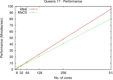
5.7.3 Performance (Million of nodes per second) - Queens (17). . . 61

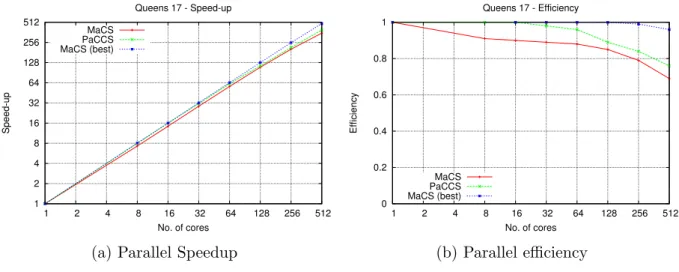
5.7.4 Scalability - Queens (17). . . 63

5.7.5 Working Time and Overhead - Golomb Ruler (n=13). . . 64

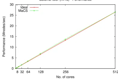
5.7.6 Performance (Million of nodes per second)- Golomb Ruler (n=13). . . 64

5.7.7 Scalability - Golomb Ruler (n=13) . . . 66

5.7.8 Working Time and Overhead - Langford’s Problem (L(2,15). . . 66

5.7.9 Performance (Million of nodes per second) - Langford’s Problem (L(2,15). 67 5.7.10 Scalability - Langford’s Problem L(2,15) . . . 68

5.7.11 Working Time and Overhead - QAP (esc16e). . . 69 xiii

(20)

5.7.12 Performance (Million of nodes per second) - QAP (esc16e). . . 69

5.7.13 Scalability - QAP (esc16e). . . 71

7.2.1 Local Search - moves along a search space . . . 83

7.2.2 Representation of local minima . . . 84

8.4.1 Communication topology . . . 106

8.5.1 Example of all-interval in music . . . 108

8.5.2 Costas Array example . . . 109

8.5.3 Magic Square 200 on 512 cores (128 nodes) . . . 111

8.5.4 Run time and length distributions - Magic Square (n=200) . . . 114

8.5.5 All Interval 400 on 256 cores (64 nodes) . . . 117

8.5.6 Run time and length distributions - All Interval (n=400) . . . 118

8.5.7 Costas Array (n=20) on 256 cores (64 nodes) . . . 120

8.5.8 Run time and length distributions - Costas Array (n=20) . . . 122

(21)

List of Tables

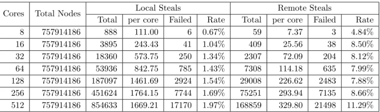
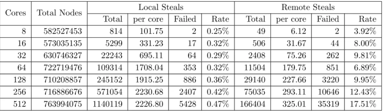
5.7.1 Work Stealing Information - Queens (n=17). . . 62

5.7.2 Work Stealing Information - Golomb Ruler (n=13). . . 65

5.7.3 Work Stealing Information - Langford’s Problem (L(2,15). . . 68

5.7.4 Work Stealing Information - QAP (esc16e). . . 70

8.5.1 Speedup for Magic Square (n=200). . . 112

8.5.2 Statistics for Magic Square (n=200). . . 113

8.5.3 Problem characteristics - Magic Square (n=200). . . 115

8.5.4 Speedup for All Interval (n=400). . . 117

8.5.5 Statistics for All Interval (n=400). . . 118

8.5.6 Problem characteristics - All Interval (n=400). . . 119

8.5.7 Speedup for Costas Array (n=20). . . 121

8.5.8 Statistics for Costas Array (n=20). . . 121

8.5.9 Problem characteristics - Costas Array (n=20). . . 122

(22)

(23)

Acronyms

API Application Programming Interface AS Adaptive Search

CBLS Constraint-Based Local Search CSP Constraint Satisfaction Problem COP Constraint Optimisation Problem

GPI Global address space Programming Interface MaCS Massively parallel Constraint Solver MPI Message Passing Interface

PaCCS Parallel Complete Constraint Solver PGAS Partitioned Global Address Space RDMA Remote Direct Memory Access UTS Unbalanced Tree Search

(24)

(25)

Chapter 1 Introduction

1.1 Motivation

Ever since it was stated, Moore’s Law has adequately described the progress of newly de-veloped processors. Before the turn of the millennium, the performance improvements of a processor were mostly driven by frequency scaling of a single processor. Still, multipro-cessor chips were already seen as a valid approach to increase performance. The focus on multiprocessor designs became clear with the diminishing returns of frequency scaling and emerging physical limitations.

The emergence of single-chip multiprocessors is a consequence of a number of limitations in today’s microprocessor design: deep pipe-lining performance exhaustion, reduced ben-efits of technology scaling for higher frequency operation, power dissipation approaching limits and memory latency. To address these limitations and continue to increase per-formance, many chip manufactures started to research and develop multicore processors. Nowadays, these are dominant and used in all kinds of platforms, from mobile devices to supercomputers.

Under this shift, the software becomes the problem since it has to be modified for par-allelism and to take advantage of a thousand or even of a million-way parpar-allelism. And this affects all layers of software, from operating systems to applications and from pro-gramming models and run-time systems to algorithms. However, parallel propro-gramming is difficult and requires real programming expertise together with a great knowledge of the underlying hardware.

In the field of high performance computing (HPC), writing parallel software is a require-ment to take advantage of supercomputers. Thus, observing the research developrequire-ments in this area can be an advantage. Moreover, a large body of knowledge on parallel computing and programming is therein concentrated.

In HPC, the most popular approach for writing parallel programs is the Message Passing Interface (MPI). MPI has been very successful but recently, researchers have started looking

(26)

2 CHAPTER 1. INTRODUCTION

for and developing alternatives.

GPI was created and continues to be developed at the Fraunhofer ITWM as an alternative to MPI. It has already proved its applicability in industrial applications provided by the Fraunhofer ITWM and its partners, in different domains such as seismic imaging,

compu-tational fluid dynamics or visualisation techniques such as ray tracing. It is a PGAS1 _API

for parallel applications running on cluster systems. GPI was created to take advantage of modern features of recent interconnects and incur in low CPU utilisation for communica-tion. Its programming model focuses on asynchronous one-sided communication, moving away from a bulk-synchronous two-sided communication pattern, an often observed pattern in parallel applications.

Notwithstanding the success and effectiveness of GPI in solving real world problems, par-allel programming is still hard specially for scientists with less background on Computer Science but with a large expertise in their domain. Moreover, applications possess different characteristics and kinds of parallelism, from which it might be straightforward or not to obtain benefit.

Declarative computational models can simplify the modelling task and are thus attractive for parallel programming, as they concentrate on the logic of the problem, reducing the programming effort and increasing the programmer productivity. The issue of how the programmer expresses its problem is orthogonal to the underlying implementation which should target and exploit the available parallelism.

Among the different declarative models, those based on constraint programming have been successfully applied to hard problems, which usually involve exploring large search spaces, a computationally intensive task, but one with significant potential for parallelisation. It is thus promising to match such declarative models with recent technologies such as GPI and study the suitability and scalability at large scale of such engagement.

1.2 Constraint Programming

Constraint Programming (CP) is one approach to declarative programming based on con-straints. In CP, a problem is modelled as a set of variables where each of them has a domain. The domain of a variable is the set of possible values it can take. Moreover, a set of relations between (some) variables is defined. This set is called the constraints of the problem. Solving a problem is thus, the assignment of a value of the domain to each variable such that no constraint is violated.

There exist different methods to solve a problem. One can distinguish between complete and incomplete methods. Complete methods always find a (best) solution or prove that no solution exists, whereas incomplete methods cannot give such guarantee. Nevertheless, incomplete methods are often very fast and return good quality solutions.

(27)

1.3. Constraint-Based Local Search 3

One of the important techniques used in complete methods is search.

Walking through a large search space looking for a solution state has a good potential for parallelisation by simply splitting the search space among different processing units, one can expect to get good speedups.

PaCCS [109]is a recent and state-of-art parallel complete constraint solver which has shown scalable performance on various problems. PaCCS explores the idea of search space split-ting among different workers and teams, implemensplit-ting techniques to ensure that all units are kept busy at all times.

1.3 Constraint-Based Local Search

Local Search is an effective technique to tackle optimisation problems and constraint sat-isfaction problems. The general idea of local search algorithms is simple: starting from an initial “candidate solution”, the algorithm performs a series of improving modifications (moves) to the current configuration until a stop criterion is met, which usually means that a solution was found.

Local Search algorithms are not guaranteed to find a (optimal) solution because they are incomplete and do not perform an exhaustive search. But they are very fast, often return good quality solutions and are able to tackle large problem instances.

Constraint-based Local Search builds on the idea of using constraints to describe and control local search. Problems are modelled using constraints plus heuristics and solutions are searched for using Local Search.

The Adaptive Search algorithm is one of many different local search methods which proved to be very efficient in the types of problems on which it was tested. Adaptive search [20, 21] is, by definition, a local search method for solving Constraint Satisfaction Problems (CSP). The key idea of the approach is to take into account the structure of the problem given by the CSP description, and to use in particular variable-based information to design general meta-heuristics.

1.4 Goals and Contributions

The main goal of this thesis is the study of declarative computational models based on constraints, with the execution on large parallel systems in mind. More specifically, we are interested in the scalability of complete constraint solving and of a constraint-based local search algorithm (Adaptive Search) when implemented to take advantage of the GPI programming model. On the other hand, we want to evaluate the suitability of GPI to such problems and the requirements of their parallel execution. To that end, different analysis and techniques for both models were implemented and are here presented.

(28)

4 CHAPTER 1. INTRODUCTION

• a GPI implementation of a scalable dynamic load balancing scheme based on work stealing, suitable for the requirements of parallel tree search and tree shaped com-putations. The implementation was evaluated on a recent system with up to 3072 cores and displayed good results and scalability.

• A parallel constraint solver, MaCS, based on the ideas of PaCCS but implemented to take advantage of the GPI programming model and leveraging the knowledge obtained with general parallel tree search. The experimental evaluation on different problems showed encouraging scalability results on a system with up to 512 cores. • A new parallel version of the Adaptive Search algorithm with GPI, including different

variants and the study of its behaviour on different problems. The study provides a deeper understanding of some scalability problems exhibited by the algorithm when executed at large scale.

Ultimately, the contributions of this thesis aim at spreading the use of declarative models based on constraints given their natural simplification of the parallel programming task and claim the establishment of GPI as a valid alternative for the implementation of constraint-based systems.

1.5 Thesis Organisation

This document is organised as follows. Chapter 2 provides the necessary context for the work presented in this thesis, with respect to parallel programming and presents GPI and its programming model.

The rest of the thesis is organised in two major parts which correspond to the two different declarative computational models we are interested in: Part I deals with the development of a parallel complete constraint solver whereas in Part II we focus on Constraint-based Local Search by exploring the Adaptive Search algorithm.

Part I includes Chapters 3 to 5. Chapter 3 introduces constraint programming and

constraint solving (including its parallelisation), providing the required background for this declarative model. Chapter 4 focuses on Parallel Search as one important aspect of parallel constraint solving and load balancing as the major obstacle to overcome. The work with the UTS benchmark is presented and the dynamic load balancing scheme based on work stealing with GPI is analysed. Chapter 5 presents MaCS, the Massively parallel Constraint Solver, based on GPI and an architecture based on that of PaCCS. It leverages the work with UTS to implement a complete constraint solver for parallel systems. Finally, Chapter 6 wraps the first part of this thesis, summarising the work presented and providing directions for future work on the topic.

Part II includes Chapters 7 and 8. In Chapter 7, we present Constraint-based Local

(29)

1.5. Thesis Organisation 5

algorithms. Chapter 8 presents the Adaptive Search algorithm and work developed towards its parallelisation with GPI, with the analysis and performance evaluation on different problems. Part II is finalised with Chapter 9 where again a summary of the work of this part is presented and different directions of research are listed.

This thesis concludes with Chapter 10 where both of its parts are put into a common perspective.

(30)

(31)

Chapter 2 Background

Modern computer architectures continue to move to increasingly parallel systems. On the software side, this trend to parallel systems implies a change towards parallel programming. This means that parallel programming is no longer a topic specific to the HPC area or only for scientists working on supercomputers.

Fortunately, there is a large amount of work on parallel computing and parallel program-ming. In this chapter we introduce some important concepts and give the necessary context for the development of the work in this thesis where GPI is a central and important point. Its features, the programming model and functionality are extensively presented.

2.1 Parallel Programming

Parallel programming is often seen as a challenging task. The programmer has the added responsibility of dealing with aspects not present when the goal is sequential execution. These include, among others, non-deterministic behaviour, load balancing and a good match to the underlying parallel computer.

When developing a parallel algorithm, the first step to be considered is to identify compo-nents that could be processed in parallel, in other words, to find concurrency in a problem in order to decompose it into sub-problems that can be independently processed in parallel. Parallelism can take different forms: with respect to the data that needs to be processed or to the different operations to be performed. Data parallelism is exhibited when the same operation is performed on the same or different elements of a data set. Task par-allelism (also know as functional parpar-allelism) is exhibited when multiple operations can be performed concurrently. These include independent parts (tasks) of a program such as function calls, basic blocks or single statements that can be run in parallel by different processors.

Most large problems contain enough concurrency to be exploited by parallel execution. Notwithstanding, their parallelisation has different requirements. Some problems require

(32)

8 CHAPTER 2. BACKGROUND

little effort to decompose them, with no dependencies and communication needs (embar-rassingly parallel ). Other problems can be partitioned statically, using domain decompo-sition techniques, with careful design to deal with data dependencies and communication. And finally, some problems depend on dynamic information where the amount of paral-lelism is initially unknown. Such problems require different and more dynamic techniques.

2.1.1 Irregular and Dynamic Problems

The development of parallel applications requires different optimisation and programming techniques to match the different types of problems. Within the whole range of problems, some possess characteristics which lead us to classify them as irregular and dynamic. Ex-amples include optimisation problems or heuristic search problems and are important in different domains such as SAT solving and machine learning.

The characteristics of such applications include unpredictable communication, unpredictable synchronisation and/or a dynamic work granularity. One common requirement is an asyn-chronous and dynamic load balancing scheme because the inherent unpredictability of the computation does not permit a static partitioning of work across the computing resources. Unpredictable communication corresponds to an execution of a program where the oc-currence of communication changes frequently. An unpredictable communication schedule raises problems to the parallel execution since sender and receiver may need to hand-shake the communication which implies a synchronisation step and possibly blocking one of the parties. Unpredictable synchronisation pattern refers to synchronisation depending on the state of the computation. It is a similar problem to the unpredictable communication. Irregular and asynchronous applications suffer from these characteristics resulting in load imbalance and waste of CPU cycles. Dynamic work granularity, where the computation depends on the input, also creates load imbalance. For example, in a search problem, each node might generate a different number of child nodes to be processed and consequently a work imbalance on each worker.

2.1.2 Performance

When solving a problem in parallel, one of the fundamental objectives is its improvement in terms of performance. One way to consider performance is as a reduction of the required execution time. Moreover, it is reasonable to expect that this execution time reduces as more processing power is employed. Scalability of a parallel algorithm is the measure of its capacity to deal with an increasing number of processing units. It can be used to predict the performance of a parallel algorithm on a large number of processors or, for a fixed problem size, determine the optimal number of processors needed and the maximum speedup that can be obtained.

For scalability analysis and understanding parallel performance in general some common definitions are required:

(33)

2.2. Parallel Programming Models 9

Speedup is the ratio of the execution time of the fastest sequential algorithm (TS) to the

execution time of the parallel version (TP).

Serial fraction is the ratio of the serial part of an algorithm to the sequential execution time. The serial part is that part of the algorithm which cannot be parallelised. Parallel overhead is the sum of the total overhead incurred due to parallel processing.

This includes communication and synchronisation costs, idle times or extra or redun-dant work performed by the parallel implementation.

Efficiency is the ratio of speedup to the number of processors (p) that is, E = TS/(pTP).

Degree of concurrency is the maximum number of tasks that can be executed simulta-neously in a parallel algorithm.

When discussing the scalability of a parallel algorithm, the speedup is the often used

metric. In the ideal case, the speedup should be linear with SP = p that is, the speedup

on p processors should equal p. Some problems can even achieve super linear speedup

where SP ≥ p. Super linear speedups happen often due to hardware related effects such

as cache effects but may also be due to the nature of the algorithm.

It is often the case, that the speedup does not continue to increase with increasing number of processors, for a fixed problem size. Amdahl [2] observed that the speedup of a parallel algorithm is bounded by 1/s where s is the serial fraction of the algorithm. This popular statement is know as Amdahl’s Law. In fact, besides the serial fraction, other factors contribute to a levelling-off or even a decrease of the speedup such as the degree of concurrency or all sorts of parallel overhead.

The problem size is important because speedup may saturate due to overhead growth or to exceeded degree of concurrency. For a fixed problem size, the parallel overhead increases with increasing number of processors, reducing the efficiency. The efficiency can be maintained if, for an increasing number of processors p, the problem size W is also increased. The rate with which W should be increased with respect to p in order to keep a fixed efficiency determines the scalability. Gustafson’s Law [58] provides a counterpoint to Amdahl’s Law in which a new metric called scaled speedup is introduced. Scaled speedup is the speedup obtained when the problem size is increased linearly with the number of processors [80].

2.2 Parallel Programming Models

A parallel programming model is an abstract view of the parallel computer, how process-ing takes place from the standpoint of the programmer. This view is influenced by the architectural design and the language, compiler or runtime libraries and thus, there exist many programming models for the same architecture.

(34)

A programming model defines how units of computation are executed and how these are mapped to the available architectural resources. This is called the execution model. The most popular execution model is the SPMD (Single Program, Multiple Data) where the same program is run by different processes which act on different (multiple) data.

A programming model also defines how data is shared. There are models with a shared, distributed address space or with a hierarchical view of it.

The most popular parallel programming models are message passing, shared memory and data parallel models. All these models have their strenghts and weaknesses which will be highlighted in this section.

In the message-passing model, several processes execute concurrently, each of them exe-cuting, sequentially, their instructions. The processes cooperate through the exchange of messages since each process only has access to its own private memory space. This message exchange is two-sided that is, there is a sender and a corresponding receiver of the message. As disadvantages, there is a considerable overhead associated with the communication, specially with small messages. And because each process has a private view of data, for large problem instances which do not fit in that private space, some extra concern with data layout and decomposition has to be introduced. This can reduce the productivity of the programmer.

In the shared memory model, multiple independent threads work on and cooperate through a common, shared address space. There is no difference between a local or a remote ac-cess. This results in greater ease of use due to its similarity to the sequential execution. The downside is that there is no control over the locality of data which could generate unnecessary remote memory accesses, degrading performance. Moreover, if the program-ming environment does not handle it, access to shared data must be synchronised to avoid inconsistencies.

The data parallel model concentrates, as the name suggests, on the data. Concurrency is achieved by processing multiple data items, simultaneously. A process operates, in one operation, on multiple data items. For example, the elements of an array to be processed in a loop can be partitioned and concurrently operated by different threads or by the use of vector instructions of the CPU. This is the case of for instance, many image processing algorithms. For applications rich in data parallelism, this model is very powerful. On the other hand, for problems with more task parallelism, this model might be less effective.

2.2.1 MPI

MPI [98] has become the de facto standard for communication among processes that model a parallel program running on a distributed memory system. It primarily addresses the message passing programming model, in which data is moved from the address space of one process to that of another process through cooperative operations on each process.

(35)

2.2. Parallel Programming Models 11

MPI is a specification, not an implementation; there are multiple implementations of MPI (OpenMPI [44], MVAPICH2 [67], MPICH [56] and others).

Notwithstanding its achievable performance and portability, two of its major advantages, the recent developments in architectural design made researchers start to question the scalability of the programming model in the pre-Exascale era.

Since its version 2.0, the MPI standard includes support for one-sided communication to

take advantage of hardware with RDMA 1 _{capabilities. Still, there are some restrictions}

which limit the applicability of MPI. These restrictions are basically related to memory access (in [11] an extensive review of these restrictions is done for the case of Partitioned Global Address Space (PGAS) Languages).

Another limitation is the implicit synchronisation of the 2-sided communication scheme, which requires both peers to participate in the information exchange even if only one of them actually needs it. This is particularly important for applications with irregular data access patterns. Also, because a sender cannot usually write directly into a receiver’s address space, some intermediate buffer is likely to be used [16]. If such buffer is small compared to the data volume, additional synchronisation occurs whenever the sender must wait for the receiver to free up the buffer.

Lastly, with the transition to multicore and manycore system designs, the process-based view of MPI maps poorly to the hierarchical structure of available hardware. Recent research results using hybrid approaches (MPI+OpenMP) are a reflex of that [72, 113]. These are of course issues of which the MPI community is well aware. Indeed, the future version of the MPI standard [22, 99] aims at addressing some of them as well as do new releases of MPI implementations.

2.2.2 PGAS

The Partitioned Global Address Space (PGAS) is another, more recent, parallel program-ming model which has been seen as a good alternative to the established MPI one. The PGAS approach offers the programmer an abstract shared address space model which sim-plifies the programming task and at the same time promotes data-locality, thread-based programming and asynchronous communication. One of its main arguments is an increased programming productivity with competing performance.

With the PGAS programming model, each process has access to two address spaces: a global and a local (private) address space. The global address space is partitioned and each partition is mapped to the memory of each node. The programmer is aware of this layout allowing her a higher control of data locality: local or in global address space; in own partition or in a remote partition.

(36)

Data in the global address space is fetched through get and put operations. These oper-ations have a one-sided semantics that is, only one side of the communication is required to invoke the communication.

The PGAS programming model is used by languages for parallel programming which aim at development productivity of parallel programs. The Unified Parallel C (UPC) [24] and Co-Array Fortran [104] are extensions of the C and Fortran programming languages respectively, which aim at high performance computing. With the same aim, X10 [18], Chapel [12], Fortress [73] are novel parallel programming languages, designed with scalable parallel applications and high programmer productivity in mind.

There has also been a substantial amount of work on communication libraries and runtime systems that support the PGAS model. ARMCI [69] is a communication library that implements RDMA operations on contiguous and non-contiguous data. The target of ARMCI though, is to create a communication layer for libraries and compiler runtime systems. For example, it has been used to implement the Global Arrays library [70] and GPSHMEM [74].

GASNet [10] is another communication library that aims at high performance. It provides network independent primitives and as for ARMCI, several implementations exist. GASNet also targets compilers and runtime systems and is used for the implementation of the PGAS languages UPC, Titanium [108] and Co-Array Fortran.

Older alternatives already exploited the same concepts (e.g. remote memory access, shared memory communication) and goals (e.g. performance). The well-known Cray SHMEM [5] library available on Cray platforms, as well as on clusters, supported put/get operations and scatter/gather operations, among other capabilities.

It is worth to note that the PGAS programming model is a variant and differs from the classical Distributed Shared Memory (DSM) and systems such as Treadmarks [76]. Under PGAS there is no coherency mechanism and it is the programmer who must care for the consistency of data. The direct control aims at, and usually results in, higher performance.

2.3 GPI

GPI2 (Global address space Programming Interface) is a PGAS API for parallel

applica-tions running on clusters [87]. It has already proved its applicability on industrial appli-cations developed by the Fraunhofer ITWM and its partners, in different domains such as seismic imaging, computational fluid dynamics or stencil-based simulations [79, 124, 57]. A crucial idea behind GPI is the use of one-sided communication where the programmer is implicitly guided to develop with the overlapping of communication and computation in mind. In some applications, the computational data dependencies allow an early request for communication or a later completion of a transfer. If one is able to find enough independent

(37)

2.3. GPI 13

computation to overlap with communication then potentially a rather small amount of time is spent waiting for transfers to finish. As only one side of the communication needs information about the data transfer, the remote side of the communication does not need to perform any action for the transfer. In a dynamic computation with changing traffic patterns, this can be very useful [6].

Its thin communication layer delivers the full performance of RDMA-enabled networks directly to the application without interrupting the CPU. In other words, as the communi-cation is completely off-loaded to the interconnect, the CPU can continue its computation. While latency could and should be hidden by overlapping it with useful computation, data movement gets reduced since no extra intermediate buffer is needed and thus, bandwidth does not get affected by it.

From a programming model point of view, GPI provides a threaded approach as opposed to a process-based view. This approach provides a better mapping to current systems with hierarchical memory levels and heterogeneous components.

In general, and given its characteristics, GPI enables and aims at a more asynchronous execution. It requires a reformulation and re-thinking of the used algorithms and commu-nication strategy in order to benefit for its characteristics. For instance, GPI does not aim at simply replacing MPI calls and provide an alternative interface for parallel programs.

2.3.1 GPI Programming Model

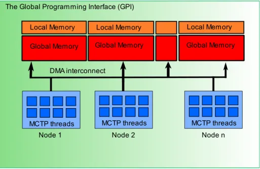
In GPI, the programmer views the underlying system as a set of nodes where each node is composed of one or more cores. All nodes are connected to each other through a DMA interconnect. This view maps, more or less directly, to a common cluster system. Figure 2.3.1 depicts the architecture of GPI.

GPI applies the SPMD execution model and each node has an identifier, the rank. The same application is started on every node and the rank is used to identify each node and for communication between nodes.

As already mentioned, GPI is a PGAS API. As in every PGAS model and from the memory point of view, each node has an internal and a global memory. The local memory is the internal memory available only to the node and allocated through typical allocators (e.g. malloc). This memory cannot be accessed by other nodes. The global memory is the partitioned global memory available to other nodes and where data shared by all nodes should be placed. Nodes issue GPI operations through the DMA interconnect.

At the node level, GPI encourages and in a sense, even enforces a thread-based model to take advantage of all cores in the system. In figure 2.3.1, each core is named a MCTP thread. MCTP, which stand for Many-Core Thread Package, is a library used with GPI and based on thread pools that abstract the native threads of the platform. Each thread has access to the local and the node’s partition of global memory as in a shared memory system. To access the global memory on a remote node, it uses one-sided communication

(38)

Global Memory

Node 1 Node 2 Node n

Local Memory

MCTP threads

Global Memory Global Memory

The Global Programming Interface (GPI)

DMA interconnect

MCTP threads MCTP threads

Local Memory Local Memory

Figure 2.3.1: GPI architecture

such as write and read operations. The global view of memory is maintained but with more control over its locality.

A thread should work asynchronously, making use of one-sided communication for data access but overlapping it with computation as much as possible. The final objective should be a full overlap of computation and communication, hiding completely the latency of communications. A secondary objective is the reduction of global communication such as barriers and their cost due to synchronisation, allowing the computation to run more asynchronously.

2.3.2 GPI Functionality

One of the most attractive features of GPI is its rather simple and short interface, pro-viding a smooth learning curve specially for someone with some background in parallel programming and/or with MPI.

GPI is constituted by a pair of components: the GPI daemon and the GPI library. The GPI daemon runs on all nodes of the cluster, waiting for requests to start applications and the library holds the functionality available for a program to use.

The GPI core functionality can be summarised as follows: • Read and write global data,

• Send and receive messages, • Passive communication, • Commands,

(39)

2.3. GPI 15

• Global atomic counters and spin-locks, • Barriers,

• Collective operations.

Two operations exist to read and write from global memory independent of whether it is a local or remote location. The important point is that those operations are one-sided and non-blocking, allowing the program to continue its execution and hence take better advantage of CPU cycles. If the application needs to make sure the data was transferred, it needs to call a wait operation that blocks until the transfer has finished, asserting that the data is usable.

GPI also supports a message-passing mode, allowing a more Send/Receive style of pro-gramming, where nodes exchange messages or commands. Exchanging messages means sending and receiving messages. For each send on one host there should be a correspond-ing receive on the other side. The send operation is non-blockcorrespond-ing allowcorrespond-ing the sender to continue computation while a receive blocks until a message arrives.

Nodes can also exchange commands. Commands are comparable to pre-defined messages that correspond to a certain request to which the receiver responds with the appropriate behaviour. The application is responsible for defining its own commands: when to send them, when to receive, what does each command mean and whether the command is a global command or targeted at/expected from a particular node.

One aspect related to all types of communication is the possibility of using different queues for handling the requests. The user provides which queue she would like to use to handle the request. These queues build on the queue pair concept of the Infiniband architecture and work similarly to a queue, in a FIFO fashion. At the moment, there exist eight such queues with 1024 entries each. These queues allow more scalability and can be used as channels for different types of requests where similar types of requests are queued and synchronised together but independently from the other requests on a different queue. The passive communication has a two-sided semantics that is, there is always a sender node with a matching receiver node. However, the receiver node does not specify the sender node for the operation and expects a message from any node. Moreover, the receiver waits for an incoming message in a passive form, not consuming CPU cycles. On the sender side the call is non-blocking but the sender is more active and specifies the node where the message should be sent. After sending the message, the sender node can continue its work, while the message gets processed by the interconnect.

Global atomic counters allow the nodes of a cluster to atomically access several counters and all nodes will see the right snapshot of the value. There are two operations supported on counters: fetch and add and fetch, compare and swap. The counters can be used as global shared variables used to synchronise nodes or events. As an example, the atomic counters can be used to distribute workload among nodes and threads during run-time. They can also be used to implement other synchronisation primitives.

(40)

Although GPI aims at more asynchronous implementations and diverging from the bulk-synchronous processing, some global synchronisation might be required. Thus, GPI imple-ments a scalable barrier at the node level. The same justifies the implementation of other collective operations such as the AllReduce that supports typical reduction operations such as the minimum, maximum or sum of standard types.

2.3.3 GPI Programming Details and Example

It is important to detail the GPI programming model and its nuances and difficulties. The two aspects which are very important to comprehend GPI and its model are the global address space and the communication primitives.

Each node contributes with a partition of the total global space (global memory in fig-ure 2.3.1). This global memory is not accessed by global references (pointers) but with the communication primitives (read /write) of GPI, the already mentioned one-sided munication, that acts over the DMA interconnect. The advantage here is that the com-munication happens without the remote node’s intervention. Thus, a global address is in fact a tuple (address, node) which is passed to the communication primitive when the data required is in a remote node. Moreover, this address is not a typical virtual address but rather an offset within the space reserved for global memory (offset, node). GPI only provides the pointer to the beginning of the global memory for each node locally.

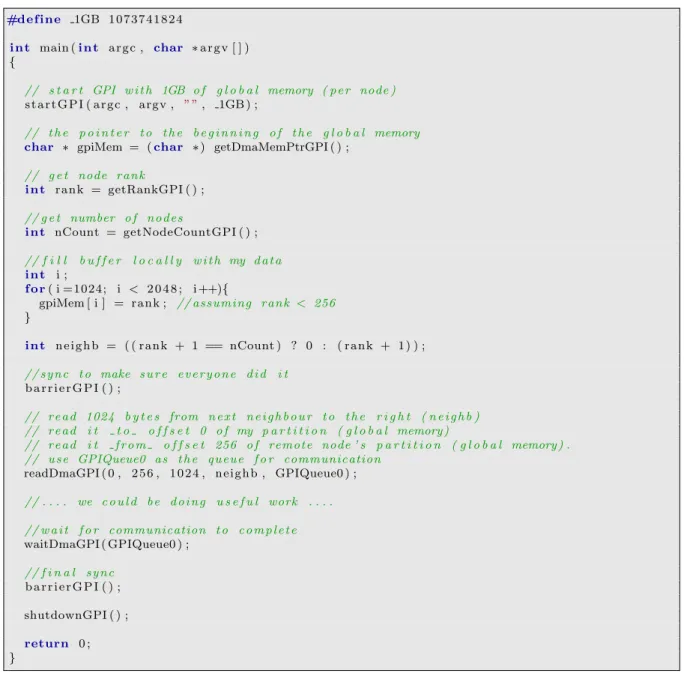
The following example illustrates the basics of GPI. At start, GPI is initialised, the size for each partition of the global memory is defined to be one Gigabyte. (For instance, if the program is executed on two nodes, the total global memory of GPI is two Gigabytes.) Then after retrieving its rank and pointer to global memory, each node will fill part of its global memory with its own rank and when everyone is finished, each node reads the filled portion of global memory directly from its neighbour. When finished, all nodes wait for each other and terminate. Note that this is one of the most basic examples possible with GPI and there are no threads at all involved (except for the main one).

The GPI global memory on each node is always present and accessible for application usage. The application must however take care of maintaining the space consistent, keeping track of where is what and to use the space wisely. For example, there is no dynamic memory allocation.

Example: Apex-MAP

One way to demonstrate the advantages of GPI is through a small example.

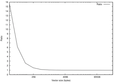
Apex-MAP [126] is an architecture independent performance characterisation and synthetic benchmark. In its version 1, the focus lies on data access. In the characterisation, the performance factors are the regularity of the access pattern, the size of the data accessed, spatial locality and temporal locality.

(41)

2.3. GPI 17

#d e f i n e 1GB 1 0 7 3 7 4 1 8 2 4

i n t main (i n t a r g c , char ∗ a r g v [ ] ) {

// s t a r t GPI w i t h 1GB o f g l o b a l memory ( p e r node )

s t a r t G P I ( a r g c , argv , ” ”, 1GB ) ;

// t h e p o i n t e r t o t h e b e g i n n i n g o f t h e g l o b a l memory

char ∗ gpiMem = (char ∗ ) getDmaMemPtrGPI ( ) ;

// g e t node r a n k i n t r a n k = getRankGPI ( ) ; // g e t number o f n o d e s i n t nCount = getNodeCountGPI ( ) ; // f i l l b u f f e r l o c a l l y w i t h my d a t a i n t i ; f o r( i =1024; i < 2 0 4 8 ; i ++){

gpiMem [ i ] = r a n k ; // assum ing r a n k < 256

} i n t n e i g h b = ( ( r a n k + 1 == nCount ) ? 0 : ( r a n k + 1 ) ) ; // s y n c t o make s u r e e v e r y o n e d i d i t b a r r i e r G P I ( ) ; // r e a d 1024 b y t e s from n e x t n e i g h b o u r t o t h e r i g h t ( n e i g h b ) // r e a d i t t o o f f s e t 0 o f my p a r t i t i o n ( g l o b a l memory )

// r e a d i t f r o m o f f s e t 256 o f remote node ’ s p a r t i t i o n ( g l o b a l memory ) . // u s e GPIQueue0 a s t h e q u e u e f o r communication readDmaGPI ( 0 , 2 5 6 , 1 0 2 4 , n e i g h b , GPIQueue0 ) ; // . . . . we c o u l d b e d o i n g u s e f u l work . . . . // w a i t f o r communication t o c o m p l e t e waitDmaGPI ( GPIQueue0 ) ; // f i n a l s y n c b a r r i e r G P I ( ) ; shutdownGPI ( ) ; return 0 ; }

Using Apex-Map, the objective was to simulate the behaviour of a shared memory seismic application. The application accesses local or remote data and performs some computation on that data. The two steps - data access and computation - are then repeated for a few iterations. In principle, the access to data that is local has a much lower latency than the access to remote data and thus, the results can be computed with a much lower execution time.

We create a GPI-based Apex-MAP implementation, by including remote memory accesses using the GPI API. Moreover, the remote accesses should be overlapped with computation in order to hide their much higher latency.

(42)

18 CHAPTER 2. BACKGROUND 0 1 2 3 4 5 6 7 8 9 10 11 12 13 14 15 16 256 4096 65536 Ratio

Vector size (bytes)

Ratio

Figure 2.3.2: Apex-MAP

set that is in a remote location with that of a local data set.

As figure 2.3.2 depicts, the ratio between both times converges to one as we increase the size of the data set. In other words, we can hide the latency of the remote access given enough computation and by using programming techniques (here, double buffering) that aim at exploiting the advantages of GPI.

2.4 Summary

This chapter introduced important concepts and tools about Parallel Computing and Pro-gramming that will be of importance in the rest of this thesis. More notoriously, GPI was introduced and related to other existing approaches to parallel programming. Its pro-gramming model, the advantages of one-sided communication and asynchronous threaded computation are the central aspects and building blocks for all the work in this thesis.

(43)

Part I

Complete Constraint Solver

(44)

(45)

21

In the first part of this thesis, we concentrate on complete constraint solving and its execution in parallel, at large scale.

We introduce Constraint Programming, discussing modelling and solving with constraints. We then concentrate on Parallel Constraint Solving identifying the candidates for paral-lelisation, focusing on the search component. One chapter is dedicated to Parallel Tree Search where we, using the UTS benchmark, design an efficient dynamic load balancing mechanism. The designed solution is applied to MaCS, a parallel constraint solver based on GPI, which we present and evaluate in detail.

(46)

(47)

Chapter 3 Constraint Programming

This chapter introduces Constraint Programming, discusses modelling and solving with constraints, and presents the necessary background on this declarative approach to pro-gramming. Given the emphasis of this work on parallelism, we discuss constraint solving from the parallelisation point of view, identifying the parts that may benefit from parallel execution and how this process has been addressed on work found in the literature.

3.1 Introduction

The idea of constraint-based programming is to solve problems by stating constraints (properties, conditions) which must be satisfied by the solution(s) of the problem and then let a solver engine find a solution. Consider the following problem as an example: a bicycle number lock [43]. You forgot the first digit but you remember a few properties about it: it is an odd number, it is not a prime number and greater than 1. With this information, you are able to derive that the digit must be the number 9.

Constraints can be considered pieces of partial information. They describe properties of unknown objects and relations among them. Objects can mean people, numbers, functions from time to reals, programs, situations. A relationship can be any assertion that can be true for some sequences of objects and false for others.

Constraint Programming is a declarative approach to programming where first a model is defined and then a solver used to find solutions for the problem.

3.2 Constraint Modelling

The first step in solving a given problem with constraint programming is to formulate it as a Constraint Satisfaction Problem (CSP). This formulation is the model of the problem.

(48)

24 CHAPTER 3. CONSTRAINT PROGRAMMING

Definition 1. A Constraint Satisfaction Problem (CSP) over finite domains is defined by a triplet (X, D, C), where:

• X = {x1, x2, . . . , xn} is an indexed set of variables;

• D = {D1, D2, . . . , Dn} is an indexed set of finite sets of values, with Di, being the

domain of variable xi for every i = 1, 2, . . . , n;

• C = {c1, c2, . . . , cm} is a set of relations between variables, called constraints.

As per Definition 1, a CSP comprises the variables of the problem and their respective domain. The domain of a variable can range over integers, reals or symbols among others but in this work we concentrate on finite domains, encoded as a finite prefix of natural numbers.

Constraint Programming is often used for and deals well with combinatorial optimisation problems. Examples are the Travelling Salesman Problem (TSP) and the Knapsack Prob-lem, two classic NP-complete problems. In such problems one aims at finding the best (optimal) solutions from a set of solutions, maximising (or minimising) a given objective function.

We can define a Constraint Optimisation Problem by extending the definition of CSP with an objective function:

Definition 2. A Constraint Optimisation Problem (COP) is defined by a 4-tuple (X, D, C, obj), where:

• (X, D, C) is a CSP and,

• obj : Sol 7→ R where Sol is the set of all solutions of (X, D, C)

A problem can have different models and their definition can be straightforward or not. Moreover, their efficiency can greatly vary. Modelling a problem with constraints is per se a task that requires expertise.

Consider the following example:

The N-Queens problem is a classical CSP example. Although simple, the N-Queens is compute intensive and a typical problem used for benchmarks. The problem consists of placing N queens on a chessboard (N x N) so that it is not possible for a queen to attack another one on the board. This means no pair of queens can share a row, a column nor a diagonal. These are the constraints of the problem.

Modelling the problem as a CSP we have:

• N variables, {x1, x2, . . . , xN}, where xi models the queen on column i

(49)

3.3. Constraint Solving 25

• the constraints:

– xi 6= xj i.e., all variables with a different value

– xi− xj 6= i − j i.e., no two queens in the first diagonal

– xi− xj 6= j − i i.e., no two queens in the second diagonal

Depending on the used environment and the level of expressiveness it allows when specifying a problem, modelling the present example (N-Queens) can be as high-level and declarative as shown by the previous informal specification. One only needs to specify the properties of the desired solution, hence the classification of Constraint Programming as a declarative paradigm.

3.3 Constraint Solving

After correctly modelling the problem at hand, a constraint solver is used to get solutions for the CSP. When solving a CSP we can be interested in finding:

• a single solution,

• all solutions or the number thereof,

• an optimal solution, in the case of solving a COP with a given objective function. A solution to a CSP is an assignment of a value from the domain of every variable, in such a way that every constraint is satisfied. When a solution for a CSP is found, we say the CSP is consistent. If a solution cannot be found, then the CSP is inconsistent. In other words, finding a solution to a CSP corresponds to finding an assignment of values for every variable from all possible combinations of assignments. The whole set of combinations is referred to as the search space.

Definition 3. Given a CSP P = (X, D, C) where D = {D1, D2, . . . , Dn}, the search

space S corresponds to the Cartesian product of the domains of all variables i.e., S = D1× D2× . . . × Dn.

A CSP can be solved by trying each possible value assignment and see if it satisfies all the constraints. However, this possibility is a very inefficient one and for many problems simply not feasible. Much more efficient methods for constraint solving exist and can be distinguished, in a first instance, between complete and incomplete methods.

Incomplete methods refer to methods that do not guarantee to find a (optimal) solution. Nevertheless, such methods often find solutions - or in case of optimisation problems, good quality solutions - and often, much faster than complete methods. This kind of algorithms is more thoroughly discussed in the second part of this thesis.

(50)

Complete methods, on the other hand, always find a (best) solution or prove that no solution exists. For that, two main techniques are used: search and constraint propagation. Search and constraint propagation can be combined in various forms. One particular class of constraint solvers combines search and constraint propagation by interleaving them throughout the solving process. At each node of the search tree, propagation is applied to the corresponding CSP, detecting inconsistency or reducing the domains of some variables. If a fix-point is achieved, search is performed. This process continues until the goal of the solving process is reached.

Propagation

One problem with using only search techniques is the late detection of inconsistency. Con-straint propagation is a technique to avoid this problem and its task is to prune the search space, by trying to detect inconsistency as soon as possible. This is done by analysing the set of constraints of the current sub-problem and the domains of the variables in order to infer additional constraints and domain reductions. The entities responsible for constraint propagation are called propagators.

Constraint propagation is executed until no more domain reductions are possible. At this point, we hit a fix-point and we say that the CSP is locally consistent.

Each time the domain of a variable has been changed, constraint propagation is usually applied. When only the domains of the variables are affected by the propagation process we call it domain propagation. If the propagation only tightens the lower and upper bounds of the domains without introducing “holes” in it, we call it bounds propagation.

Search

With search, a problem is split into sub-problems which are solved recursively, usually using backtracking. Backtracking search incrementally attempts to extend a partial assignment toward a complete solution, by repeatedly choosing a value for another variable and keeping the previous state of variables so that it can be restored, should failure occur. Solving a CSP is therefore, the traversal of a tree whose nodes correspond to the sub-problems (partial assignments) and where the root of the tree is the initial problem with no assignments. An important aspect is the order in which variables and values are considered. The effi-ciency of search algorithms such as backtracking, that attempt to extend a partial solution, depends on these orders. The order of variables and the values chosen for each variable affects the execution time and shape of the search tree and may have a different effect on different problems. There exist various heuristics for ordering of values and variables. An example of a variable ordering heuristic is most constrained where the variable which appears most in the constraints is ordered least. In the case of value ordering, one example is the random value which orders values randomly.

(51)

3.4. Parallel Constraint Solving 27

Another important aspect is how the domain of a variable is split. Here too there exist different procedures. For example, bisection divides the values in a variable domain into

two equal halves i.e., for a domain D = d1, d2, ..., dn, bisection splits the domain into

{d1, d2, ..., dk}, {dk+1, ..., dn} where k = bn/2c. Another example is labelling, where the

domain D is split into {d1}, {d2, ..., dn}.

The last relevant aspect related to search is the search strategy. It defines how the search tree should be traversed. Starting from a node, the process decides how to proceed to one of its descendants. For example, in depth-first search (DFS), the procedure starts at the root node, descending to the first of its descendants until it reaches a leaf node i.e., a node with no descendants. When this leaf node is reached, it backtracks to the parent node and descends again to the next descendant. This procedure is repeated until all leaf nodes have been visited and the procedure has returned to the root node.

Optimisation Problems

Solving a Constraint Optimisation Problem (COP) can be performed solely by using con-straint solving techniques, taking the COP as a single CSP or a series of CSPs. In the former case, the COP is solved by finding all the solutions of the problem and choosing the one that better fits the objective function. In the latter case, several CSPs are solved by setting the domain of the constrained variable of the objective function to the smallest possible value. The value is then increased gradually until a solution is found. This applies to a minimisation problem but is easily applied to a maximisation problem where, instead of starting with the smallest value, the largest value is set and then gradually decreased. The problem with both approaches is the generation of redundant work. A more efficient and popular algorithm for solving COPs is the branch-and-bound general algorithm [83]. With this algorithm, large parts of the search space are pruned by keeping the best solution (bound) found during the process, using it to evaluate a partial solution. If a partial solution does not lead to a better solution, when compared with the current bound, that part of the search space is avoided and left unexplored.

3.4 Parallel Constraint Solving

Due to the declarative nature of Constraint Programming, taking advantage of parallelism should be achieved at the solving step. The modelling step should remain intact as well as the user’s awareness of the underlying implementation.

Parallelising Constraint Solving is, as in all kinds of algorithms and applications, a matter of identifying parts that can take advantage of parallel execution. In the literature, the parallelisation of constraint solving has faced many approaches where the different parts of the process have been experimented with.

(52)

The first obvious candidate to parallelisation is propagation where several propagators are evaluated in parallel. For problems where propagation consumes most of the computation time, good speedups may be achieved if propagation is executed in parallel. On the other hand, the overhead involved due to synchronisation and the fine grained parallelism can limit the scalability. The implementation of parallel constraint propagation involves keep-ing the available work evenly distributed among the entities responsible for propagation and guarantee that the synchronisation overhead is low.

The other obvious and most common approach found in the literature is to parallelise the search. Search traverses a (virtual) tree, splitting a problem into one or more sub-problems that can be handled independently and thus, in parallel. The scalability potential of tree search is encouraging, specially when the interest is large scale. However some challenges are unavoidable and since it is one of the main focus in the work of this thesis, we provide more details in Chapter 4.

Besides the two most obvious parts mentioned before, other approaches are possible. One is the use of a portfolio of strategies and/or algorithms where different strategies are started in parallel on the same problem. The reasoning behind this approach is that with this variety of strategies, it is to expect that one of them will outperform the others. As more parallel power is employed (and consequently more strategies) the probability that the best strategy is used, increases. This is a often and successfully used approach within the SAT solving community [135, 60]. Another approach is to distribute the variables and constraints among agents, where each agent is responsible for its own portion of the CSP. Constraints are local if they only involve variables local to the agent and are non-local if they involve variables belonging to different agents. Each agent instantiates its local variables in such way that local constraints are satisfied and non-local constraints are not violated. When an agent finds a solution, it sends a partial assignment to other agents that need to check their non-local constraints. This approach is usually referred as Distributed Constraint Satisfaction and the problems are referred as Distributed Constraint Satisfaction Problems (DisCSPs) [140, 141].

3.4.1 Related Work

Parallelism in CP has focused mainly on parallel search, although propagation (consistency) has also received some attention.

The research in parallel consistency has mostly focused on arc-consistency even when it has been shown to be inherently sequential [75]. Still, a great portion of research in the 90’s has been produced, resulting in new algorithms and results [142, 103, 120, 121]. After that, in 2002, [59] presented DisAC-9, an optimal distributed algorithm for performing arc-consistency which focuses on the number of passed messages. More recently, parallel consistency has again received some interest in the work of Rolf [118, 119]. Specifically, their work studies parallel consistency with global constraints. In [119] the authors extend the work with parallel consistency with parallel search, combining both.

Massivel y parallel declarative computational models

MASSIVELY PARALLEL DECLARATIVE

COMPUTATIONAL MODELS

Rui Mário da Silva Machado

UNIVERSIDADE DE ´

EVORA

Massively Parallel Declarative

Computational Models

Rui M´

ario da Silva Machado

´

Acknowledgments

Abstract

Modelos de Computa¸

c˜

ao Declarativos

Massivamente Paralelos

Sum´

ario

List of Publications

Contents

I

Complete Constraint Solver

19

II

Parallel Constraint-Based Local Search

77

List of Figures

List of Tables

Acronyms

Chapter 1

Introduction

1.1

Motivation

1.2

Constraint Programming

1.3

Constraint-Based Local Search

1.4

Goals and Contributions

1.5

Thesis Organisation

Chapter 2

Background

2.1

Parallel Programming

2.1.1

Irregular and Dynamic Problems

2.1.2

Performance

2.2

Parallel Programming Models

2.2.1

MPI

2.2.2

PGAS

2.3

GPI

2.3.1

GPI Programming Model

2.3.2

GPI Functionality

2.3.3

GPI Programming Details and Example

2.4

Summary

Part I

Complete Constraint Solver

Chapter 3

Constraint Programming

3.1

Introduction

3.2

Constraint Modelling

3.3

Constraint Solving

Propagation

Search

Optimisation Problems

3.4