Universidade de Aveiro Departamento de Eletrónica, Telecomunicações e Informática 2012/2013
Daniel Augusto
Santos
Modelos cranianos 3D: nova abordagem
craniométrica
“He who would learn to fly one day must first learn to walk and run and climb and dance; one cannot fly into flying.”
— Friedrich Wilhelm Nietzsche Universidade de Aveiro Departamento de Eletrónica, Telecomunicações e Informática 2012/2013
Daniel Augusto
Santos
Modelos cranianos 3D: nova abordagem
craniométrica
Universidade de Aveiro Departamento de Eletrónica, Telecomunicações e Informática 2012/2013
Daniel Augusto
Santos
Modelos cranianos 3D: nova abordagem
craniométrica
3D skull models: a new craniometric approach
Dissertação apresentada à Universidade de Aveiro para cumprimento dos re-quisitos necessários à obtenção do grau de Mestre em Sistemas de informa-ção, realizada sob a orientação científica do Doutor Paulo Miguel de Jesus Dias, Professor Auxiliar do Departamento de Eletrónica, Telecomunicações e Informática da Universidade de Aveiro, e da Doutora Maria Beatriz Alves de Sousa Santos, Professora Associada c/ Agregação do Departamento de Eletrónica, Telecominicações e Informática da Universidade de Aveiro.
Dedico este trabalho à minha falecida avó, Amélia
da Conceição.
o júri / the jury
presidente / president Prof. Doutor José Manuel Matos Moreira
Professor Auxiliar da Universidade de Aveiro
vogais / examiners committee Prof. Doutor Jaime dos Santos Cardoso
Professor Auxiliar da Faculdade de Engenharia da Universidade do Porto
Prof. Doutor Paulo Miguel de Jesus Dias
Professor Auxiliar do Departamento de Eletrónica, Telecominicações e Informática da Universi-dade de Aveiro
Prof. Doutora Maria Beatriz Alves de Sousa Santos
Professora Associada c/ Agregação do Departamento de Eletrónica, Telecominicações e Infor-mática da Universidade de Aveiro
agradecimentos / acknowledgements
Agradeço ao Professor Carlos Ferreira do Departamento de Economia, Gestão e Engenharia Industrial da Universidade de Aveiro pelos testes feitos no âmbito da estudo com PCA - Principal Components Analysis
Agradeço ao Hélder Santos (Morph), Catarina Coelho (Styx), Maria Te-resa Ferreira (iDryas, Grupo Dryas Octopetala, Coimbra, Portugal; Forensic Sciences Centre, Coimbra, Portugal), Eugénia Cunha (Forensic Sciences Centre, Coimbra, Portugal; Life Sciences Department, Faculty of Sciences and Technology, Univ. Coimbra, Portugal; Portuguese National Institute of Legal Medicine, South Branch, Coimbra, Portugal) e Miguel Almeida (iDryas, Grupo Dryas Octopetala, Coimbra, Portugal) pela constante disponibilidade e cooperação.
Agradeço ao meu orientador, Paulo Miguel de Jesus Dias, e à minha co-orientadora, Maria Beatriz Alves de Sousa Santos, por toda a ajuda gentilmente oferecida.
Palavras Chave Craniometria, Modelos 3D, Aquisição 3D
Resumo Esta dissertação apresenta uma nova abordagem para realizar análises crani-ométricas com base em modelos 3D de crânios. Atualmente o procedimento usado pelos antropólogos assenta no recurso a craniometria tradicional, i.e. medições manuais, o que implica variados problemas tais como dificuldade em assegurar repetibilidade das medições, erros na mesmas e possível dano nos crânios inerente ao seu manuseamento. A abordagem proposta passa por fazer a aquisição dos crânios recorrendo a um scanner 3D de luz estrutu-rada (realizada por terceiros) e posterior análise recorrendo a uma aplicação especificamente desenvolvida para tal, e na qual assenta o trabalho descrito neste documento. Vários métodos serão abordados, tais como análise de ma-lhas 3D, estudos de normais e curvaturas, obtenção de pontos de interesse e respectivas medidas e, por fim, serão apresentadas conclusões sobre o trabalho, bem como sugestões de trabalho futuro.
Keywords Craniometry, 3D Models, 3D Acquisition
Abstract This dissertation presents a new approach to conduct craniometric analysis based on 3D models of skulls. Nowadays procedures used by anthropologists are based in traditional methods, i.e. manual measurements, which may imply a set of problems such as difficulty in ensuring repeatability of the measure-ments, measurement errors and can skull damage inherent to the handling. The new approach lies on the acquisition of the skulls using a structured 3D light scanner (done by a third party entity) and subsequent analysis using an application specifically designed for that purpose. Is on the latter that this work is based. Several methods are going to be addressed, such as analysis of 3D meshes, studies of normal vectors and curvatures, obtainment of points of interest (landmark points) and measurements. Finally, conclusions about the developed methods, results and future work.
Contents
Contents i
List of Figures iii
List of Tables v
1 Introduction 1
1.1 Motivation and Objectives . . . 2
1.1.1 Craniometry . . . 2
1.1.2 Similar Applications and Studies . . . 3
1.2 Document Structure . . . 4
2 Traditional Craniometric Analysis and Tools 5 2.1 Case Study . . . 5
2.2 3D Scanning . . . 6
2.3 Skulls Acquisition . . . 8
2.4 Points and Measures of Interest . . . 10
3 Application - CraMs 13 3.1 Architecture . . . 13
3.2 Programming Language and APIs’ . . . 15
3.3 Alignment . . . 15 3.3.1 Related Work . . . 15 3.3.2 Manual Alignment . . . 17 3.3.3 Automatic Alignment . . . 18 3.3.4 Semi-automatic Alignment . . . 20 3.3.5 Discussion . . . 23
3.4 Methods - Neighbouring and Area Selection . . . 23
3.4.1 Points . . . 25
3.4.2 Measures . . . 27
3.5 Curvature and Normal Analysis . . . 28
3.5.1 Introduction . . . 28 3.5.2 Normal Analysis . . . 30 3.5.3 Curvature Analysis . . . 31 3.5.4 Work Flow . . . 35 3.5.5 User Interface . . . 35 3.5.6 Points . . . 37 3.5.7 Measures . . . 38 4 Results 41 4.1 Overview . . . 41
4.2 Results from the Alignment Approaches . . . 42
4.3 Results from the Curvature Analysis . . . 43
4.4 Craniometric Results and Discussion . . . 43
4.5 Inter-observer Evaluation with iDryas Experts . . . 44
5 Conclusion and Future Work 49 5.1 Conclusion . . . 49
5.2 Future Work . . . 50
Bibliography 53
Appendix A Points 57
Appendix B Measures 65
Appendix C Measurement Tables for All (8) Skulls 69
List of Figures
2.1 Example of structured light scanning system . . . 7
2.2 Breuckman 3D Scanner . . . 9
2.3 Acquired skull from the Breuckman Smartscanner - proprietary software . . . . 10
3.1 Work flow of the application . . . 13
3.2 Application architecture . . . 14
3.3 The craniometric planes . . . 17
3.4 Scatterplot for the original coordinates - variables A and B . . . 19
3.5 Scatterplot for the original coordinates - variables A and C . . . 19
3.6 Scatterplot for the original coordinates - variables B and C . . . 19
3.7 Eigenvalues of the correlation matrix (active variables only) . . . 20
3.8 Eigenvectors of the correlation matrix (active variables only) . . . 20
3.9 Factor coordinates of the variables (based on correlations) . . . 20
3.10 Variables projection on the factor plane 1x2 . . . 20
3.11 Variables projection on the factor plane 1x3 . . . 20
3.12 Variables projection on the factor plane 2x3 . . . 20
3.13 Unaligned model . . . 22
3.14 Model to align and template model (blue) . . . 22
3.15 Model aligned - ICP was successful . . . 22
3.16 Unaligned model . . . 22
3.17 Model to align and template model (blue) . . . 22
3.18 Model aligned - ICP algorithm has failed . . . 22
3.19 Neighbouring algorithm applied to the nasion . . . 24
3.20 Glabella detection using the 3D box widget . . . 25
3.21 Points automatically found . . . 26
3.23 Zero (aprox.) Curvature . . . 30
3.24 Positive Curvature . . . 30
3.25 Curvature analysis - ellipsoidal mesh . . . 31
3.26 Normal analysis - ellipsoidal mesh . . . 31
3.27 Normal analysis . . . 33
3.28 Mean curvature . . . 33
3.29 Gaussian curvature . . . 34
3.30 Work flow of the application . . . 35
3.31 Obtained points with the help of all the developed methods (including curvature) 38 3.32 Obtained measures . . . 39
1 Skull back . . . 58
2 Skull down . . . 59
3 Skull down inside . . . 60
4 Skull front . . . 61
5 Skull side . . . 62
6 Skull top . . . 63
7 CMake GUI configuration tool on Windows . . . 74
List of Tables
3.1 Facial Width . . . 28 3.2 Height of the skull . . . 28 3.3 Length of the base of the skull . . . 28 4.1 Comparison of the automatic measures obtained using manual and ICP based
alignment. Units are mm . . . . 42 4.2 Automatically obtained points from the application of local extremes (minimum or
maximum) with and without the help of curvature analysis to refine the obtained points of interest. Units are mm . . . . 43 4.3 Results - Comparison of the measures obtained from the application and by the
experts mm . . . . 44 4.4 Results from two domain experts using the developed application. Units are mm 45 4.5 The variation (inter-observer) of the measures using the application (App) and
traditional methods by the experts (iDryas). The variation was calculated taking in account two measurements of different uses, for each case. Attempts to provide a simple comparison of inter-observer error indicator. Units are mm . . . . 46 4.6 Relative TEM (mm) . . . . 47
1
Introduction
T
his dissertation is a collaboration between IEETA1, the company Dryas Archaeology2, and CENCIFOR3. It presents a new approach to perform craniometric analysis from digital models, resulting of the acquisition process with a 3D structured light scanning system, instead of direct manipulation of the original skulls. The document will describe the researched and developed methods and tools on the subject and, as well, the obtained results and conclusions.
Craniometric analysis is the main tool used in Anthropology to identify gender, ancestry and variations in populations [1]. The determination of these characteristics is typically per-formed using traditional craniometric measurements (physically measured in the skulls)[2], [3]. These traditional techniques suffer from several drawbacks: poor repeatability (intra-and inter-observer errors), impossibility to perform on fragments (intra-and/or in fragmented skulls, inadequacy to describe complex shapes and the need for actual contact with the skulls that may damage the bones. The question of bones damage is of crucial importance since, once the damage is done, some information may have been lost forever and, consequently, the opportunity to use the data to discover something relevant.
The main objective of this thesis was the development of (software) tools to make possible, from the acquired 3D models, the calculation of the principal craniometric measures used by anthropologists to caracterize the skulls.
The initially defined objectives were following:
1. Study of the relevant topics in the craniometry science and work already done on this field. 1http://www.ieeta.pt/ 2 http://www.dryas.pt/ 3 http://www.cencifor.org/
2. Development of software tools to obtain craniometric measures automatically/semi
automatically/manually.
3. Comparison (and validation) of the obtained results with the ones obtained from the traditionally used (manual) methods.
1.1 Motivation and Objectives
1.1.1 Craniometry
T
he applicability of craniometry to anthropological research, as a diagnostic tool for gender and ancestry estimation, and human evolution studies is well known [2], [4]–[7]. The roots of anthropometry are traced back to the measurement of the skull by early scien-tists [2]. Simply defined, craniometry refers to the study of human cranial measurements for use in anthropological classification and comparison [2].The protocol for gender and ancestry estimation by visual assessment of non metric traits typically involves the extraction of each feature of the skull and then sorting them into cate-gories previously defined based on shape and size differences [2], [6], [8]–[10]. However, such approach has been largely criticized for being highly subjective [7]–[12]. Citing Hefner [8]: "The experience based method of ancestry prediction using morphoscopic traits indeed is an art: an art that is intuitive, untestable, unempirical, and consequently unscientific. It is often more appropriate to perform a metric analysis when working with morphological data, since it has proven to be more objective". Because measurements rely on standard landmarks, results exhibit lower levels of intra- and inter- observer errors [2], [9], [10]. Similarly there are more powerful statistical methods for the analysis of continuous data. Linear measurements are commonly evaluated by uni- and multivariate statistical analysis, like discriminant functions [2], [6], [13], [14]. Nevertheless, traditional linear measurements are not able to capture the shape differences of some complex and rounded structures, e.g. orbit shape [7], [12]. Because of that, with a greater emphasis put on shape rather than size, visual assessment method-ologies provided the most appreciated way to assess shape differences, at least until recently [2], [9], [10], [12]. A major change started at the ending of last century. Data regarding the geometry of the morphological structure employing 3D coordinates of anatomical landmarks were of particular interest, and methods to analyze such data started to be developed [6], [7], [9], [10], [15]. This approach offers some advantages in relation to linear measurements. Investigators can preserve geometric information about the relative positions of coordinated points, visualize results of multivariate analyses as configurations of landmarks back in the original space of the organism, and assess variation in structures with few or no landmarks
[5]–[7], [9], [10]. Thus, geometric morphometrics would be more appropriate to describe differences in structures related with gender, ancestry and human variation.
1.1.2 Similar Applications and Studies
T
o the best of the authors’ knowledge, no other tool (or set of tools) with the desired functionality exist. That fact adds more importance to the work developed since, besides its applicability, it is a new approach, and that can make the difference in terms of innovation introduced. The possible downside is that not existing any software to compare with, might be somewhat difficult to make a set of tools that can be easily used by non IT specialists. That relates, essentially, to their usability. On the other hand, it is positive in the way that with no comparisons to make, there was a greater freedom to develop the tools following the anthropologists needs.There are some other studies in the forensic science, mainly in the skull reconstruction and feature extraction, in order to obtain information about age, gender, nutritional status or even general level of health. One of those studies was made by Park et al[16]. They used scanners with laser technology to make the acquisition of the skulls with the help of an attached stylus to record the position and orientation. Their goal was to investigate the intra- and inter-examiner reliability when using a laser scan to acquire skulls, i.e. be used in craniometry analysis, and compare the results with the traditionally obtained (manually) by the specialists. It must be noted that, in their work, no landmark points detection was created. The points of interest were all indicated (with a stylus), method similar to manually picking all of the feature points. They have concluded that the method was very useful and with excellent intra- and inter-reliabilities for craniometric studies. This procedure, at least as the literature is concerned, is the choice to make acquisition, with some appended extra information, used to make craniometric studies.
Other studies were made on a topic not directly related (and not derectly aplicable) to cranimetric studies, but still relevant: the model alignment. The alignment, as will be explained later on the document, has an important role on the subject. One method was presented by Chaouch et al [17], based on the analysis of the reflective symmetry and the local translational symmetry along a direction. They have concluded that the proposed method was able to find a rotation that best aligns the 3D models in analysis. This method must be considered as of general use, i.e. for any type of 3D shapes.
Another study, and still considering the alignment of the models, was made by Cheng et al[18]. They focused in the automatic identification of two craniometric planes to, as a further step, automatically align the 3D models. The two planes were the Frankfurt and Saggital, since both planes are used to define important landmarks on the skull. Procedurally, they have
registered a template skull model with known landmarks (both planes) to a target skull in order to make the mapping. Then, the algorithm iteractively refined the landmark locations according to their medical definition, aiming the best accuracy possible. They concluded that the method was more accurate than symmetry-based methods.
1.2 Document Structure
T
his document is structured in three main sections, besides this chapter.The first part (chapter 2) is devoted to the description of the craniometry as a science and method, the points and, as well, the measures of interest to make the characterization of the models under study.
Throughout the second part (chapter 3) the complete implementation process is explained. Topics as the technologies through the development process, the chosen architecture for the application, user interface and algorithms of the software are covered.
Finally, there is a third part (chapters 4 and 5) focused on the obtained results, teir discussion and conclusions.
2
Traditional Craniometric Analysis and Tools
T
his chapter is devoted to the analysis of the case study, reference to the tools currently used by the anthropologists, description of some inherent concepts relative to the tech-nologies used on the acquisition process and a brief description of the points and measures of interest.2.1 Case Study
I
n 2009, a iDryas team performed a rescue excavation at Vale da Gafaria (Leprosarium Valley), a site located outside the medieval and modern walls of the Portuguese city of Lagos [19], [20]. This site (15-17th centuries) revealed two occupations. Part of Lagos Leprosarium, only known from historical documents, was excavated. The related necropolis was also identified, with 11 individuals recovered [19], [20]. But, the most significant occu-pation was an urban discard deposit with an area of more than 1500m2and a stratigraphic thickness superior to 6 meters. Among discarded objects, an important amount of human remains were exhumed (155 individuals, including children).
The skulls collection is composed by 65 cranial and mandibular remains of 60 slaves and 4 leprosy suffers. All of them had an age of death superior to 18 years old. From the 64 remains, 20 are from males, 30 from females and 14 were not determined. Also, worth of mention, is the preservation: 38% have the skulls and mandibles complete, 14% were manually reconstructed (by the anthropologists team) and 48% were fragmented. The frag-mentation leaded to the missing of some anatomical portions, and represents an additional challenge (as it will be described later in the text).
Considering the worldwide lack of osteoarchaeological series that could illustrate the ear-liest phase of the European Atlantic expansion [8], the preliminary research results obtained from the Lagos site are a pioneering attempt to characterize African slaves. The vast majority of the excavated necropolises relevant for the history of the modern Atlantic commerce of African slaves dates from later periods (17th-19th centuries) and was found in the New World [21]. Moreover, only occasionally have the anthropological analyses of African slaves’ popu-lations been extensive [8]. Furthermore, only direct observation of the osteological specimens was performed, 3D imaging techniques proposed in this project are unprecedented.
2.2 3D Scanning
T
hreedimensional scanning is nowadays an established technology, capable of producing high precision tridimensional digital models for documentation of the reality throughReversed Engineering, thus being particularly adapted to cultural heritage remains
docu-mentation [22], [23]. Reversed Engineering provides powerful, non-destructive R&D tools for the objects’ microscopic analysis, allowing a rigorous measurement of their features, surface geometry, texture and volume, using virtual examination, i.e. not requiring repetitive contact with their surface. The preservation of the objects’ original physical integrity is especially important in fragile human osteoarchaeological remains. Moreover, this technique also induces the development of new multidisciplinary scientific collaborations, as it allows the swift dissemination of the information, even to geographically distant researchers.
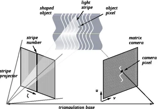
A 3D scanner is a device that analyzes a real-world object or environment to collect data on its shape and possibly its color. The collected data can then be used to construct digital three dimensional models. The purpose of a 3D scanner is usually to create a point cloud of geometric samples on the surface of the subject. These points can then be used to extrapolate the shape of the subject (a process called reconstruction). If color information is collected at each point, then the colors on the surface of the subject can also be registered. 3D scanners share several traits with cameras. Like cameras, they have a cone-like field of view, and like cameras, they can only collect information about surfaces that are not occluded. While a camera collects color information about surfaces within its field of view, a 3D scanner collects distance information about surface within its field of view. The picture produced by a 3D scanner describes the distance to a surface at each point in the picture. This allows the three dimensional position of each point, in the picture, to be identified. Figure 2.1 shows a setup of a structured light scanning system.
For most situations, a single scan will not produce a complete model of the subject. Multiple scans from many different directions are usually required to obtain information about all sides of the subject. These scans have to be brought in a common reference system, a process
Figure 2.1: Example of structured light scanning system
that is usually called registration, and then merged to create a complete model[24].
There are a variety of technologies for digitally acquiring the shape of a 3D object. A well established classification[25] divides them into two types: contact and non-contact 3D scanners.
Non-contact 3D scanners can be further divided into two main categories, active scanners and passive scanners.
• Contact: probe the subject through physical touch, while the object is in contact with or resting on a precision flat surface plate or on the ground.
• Non-contact:
– Active: emit some kind of radiation or light and detect its reflection or radiation passing through the object in order to probe an object or environment. Possible types of emissions used include light, ultrasound or x-ray.
– Passive: do not emit any kind of radiation themselves, but instead rely on de-tecting reflected ambient radiation. Most scanners of this type detect visible light because it is a readily available ambient radiation. Other types of radiation, such as infrared could also be used. Passive methods can be very cheap, as in most cases they do not need particular hardware but simple digital cameras.
A structured 3D light scanner is a non contact, active device for measuring the three-dimensional shape of an object using projected light patterns and a camera system[26]. Two main methods are mostly used:
1. Projecting a narrow band of light onto a three-dimensionally shaped surface. That produces a line of illumination that appears distorted from other perspectives than that of the projector, and can be used for an exact geometric reconstruction of the surface shape (light section).
2. A faster and more versatile method is the projection of patterns consisting of many stripes at once. This allows for the acquisition of a multitude of samples simultaneously. Seen from different viewpoints, the pattern appears geometrically distorted due to the surface shape of the object.
Although many other variants of structured light projection are possible, patterns of parallel stripes are widely used2.1. The picture shows the geometrical deformation of a single stripe projected onto a simple 3D surface. The displacement of the stripes allows for an exact retrieval of the 3D coordinates of any details on the objects’ surface.
Two major methods of stripe pattern generation have been established: Laser interference and projection.
1. Laser: the laser interference method works with two wide planar laser beam fronts. Their interference results in regular, equidistant line patterns. Different pattern sizes can be obtained by changing the angle between these beams. The method allows for the exact and easy generation of a very fine pattern with unlimited depth of field. Disadvantages are high cost of implementation, difficulties providing the ideal beam geometry, laser typical effects as noise and the possible self interference with reflection from other objects.
2. Projection: the projection method uses non coherent light and basically work as a video projector. Patterns are generated by a display within the projector, typically an LCD (liquid crystal) or LCOS (liquid crystal on silicon) display.
An essential procedure is the calibration to compensate geometric distortions by optics and perspective. The methods consists in using special calibration patterns and surfaces resorting in mathematical models to describe the imaging properties of projector and cameras.
2.3 Skulls Acquisition
T
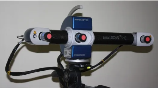
heacquisition of the 3D skull models on this project was performed using a structured light scanner (Breuckmann Smartscan see Figure 2.2). The acquisition was done by a team from iDryas, including 3D acquisition technician and athropologists, to ensure that important sections of the skulls are acquired and to define a methodology that can be easily repeated in the future. The scanner is sensitive to natural light so the scans were digitizedFigure 2.2: Breuckman 3D Scanner
under controlled light conditions.
A methodology was refined in order to acquire as much detail as possible with as few scans as possible. Most of the scans are made from an inferior view of the skull, specifically the teeth area. As the scanner works in stereo mode there is a limitation on the depth of the acquired surface.
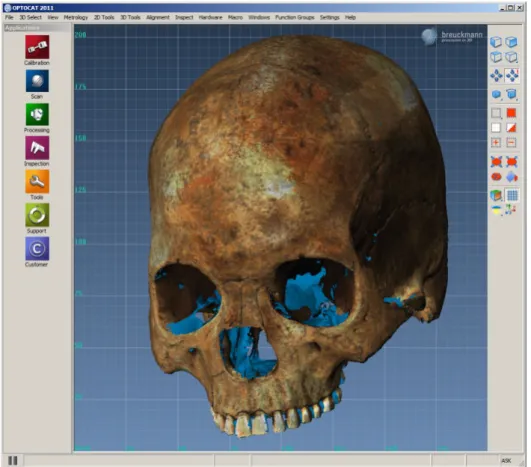
Proprietary (software) application of the sensor was used to register all range images and texture images together to provide a complete 3D model of the skull under study. Figure 2.3 shows a skull resulting from an acquisition. This model was processed from 21 scans with the 3D sensor. The final textured triangular mesh is composed of about 1.5 million triangles with an error below 30 µm and is encoded using the PLY (polygon) file format. The PLY format describes an object as a collection of vertices, faces and other elements, along with properties such as color and normal direction that can be attached to these elements. It allows to store some properties related to the object like color, surface normals, texture coordinates and transparency. The expected error depends mainly on lighting conditions and characteristics of the surface being scanned.
Figure 2.3: Acquired skull from the Breuckman Smartscanner - proprietary software
2.4 Points and Measures of Interest
D
efiningthe points of interest to be further used to compute the measures is an essencial requirement. In craniometry many craniometric points are well defined and established as standard use for classification. The anthropologists at iDryas have defined, from the set of points aforementioned, a total of 16 points (see appendix A to get a full list and description) as being of interest for the intended classification. With those 16 points they could get a total of 20 measures (see appendix B for more detail) to be later used to skul classification.The measuring system, following the traditional methodologies, is always susceptible to the introduction of some error on the measures. Observational error (or measurement error) is the difference between a measured value of quantity and its true value [27]. During the manual analysis of the skulls two typed of errors must be considered:
1. Inter-observer error: the differences between interpretations of two or more individuals making observations of the same phenomenon.
2. Intra-observer error: the differences between interpretations of an individual making observations of the same phenomenon at different times.
As previously mentioned, one of the main expected benefits in developing a method of acquisition and further digital analysis of the skulls is to assure repeatability of the results and, at same time, reducing the measurement error. Also, if possible (what it is firmly believed), reduce the (inter- and intra- observer) variability introduced by the (multiple) manual measurements.
The iDryas team has been using the FORDISC [28] software to classify the skulls. FORDISC is an interactive discriminant functions software created by Stephen Ousley and Richard Jantz [28], widely used by forensic anthropologists to assist in the creation of a dece-dent’s biological profile when only parts of the cranium are available. The program compares potential profiles to data contained in a database of skeletal measurements of modern hu-mans. The functionality falls in the classification of unknown adult skulls on its ancestry, sex and height based on the reference samples which are stored in a database. Discriminant functions are used to construct a classification matrix, and thereby attempts to reach the population group that has more similarities with the unknown individual.
3
Application - CraMs
3.1 Architecture
T
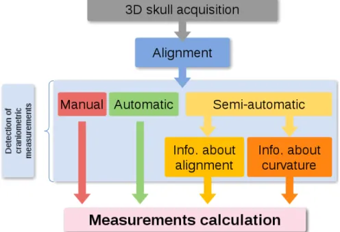
he developed application, stands for CraMs, is conceptually organized according to figure 3.1. The acquisition process of the skulls follows the procedure explained in Section 2.1. After loading the 3D model, it is necessary to align it. This procedure can be fully manual or semi-automatic. With the aligned model, it is possible to detect some craniometric points of interest. The developed methods allow manual, semi-automatic and fully automatic selection of landmark points. Finally, based on points obtained, the measuresFigure 3.1: Work flow of the application
software like FORDISC[28].
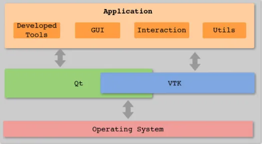
Figure 3.2 shows a brief but concise view of how the application is structured. Both VTK and Qt are on the top of the Operating System specific code (endianess, file system, etc). Messages are exchanged between both VTK and Qt in order to make possible the APIs’ integration (interaction, visualization, windowing system, etc). Concurrently, messages are exchanged between both APIs’ and the Operating system (system calls) to make possible the handling of platform specific tasks. The application is on top of both APIs’ in use and information is exchanged relatively to the GUI, interaction, visualization, etc. The application layer shows the distinction between four modules:
1. Developed tools: the methods developed to analyse the models, find points of interest, take care of the alignment, etc.
2. GUI: the graphical user interface containing all of the Qt code to handle the window creation, menus, etc.
3. Interaction: contains the code to handle the interaction with the loaded models. Widely used VTKs’ functionality.
4. Utils: some utility classes and functions.
3.2 Programming Language and APIs’
T
he application was developed using the C++ Programing Language. Qt was used for the user interface and VTK for the 3D visualization and interaction. Currently, the application runs on both MicrosoftTMWindows and GNU/Linux Operating Systems.R
Since the building system relies on CMake and the code was written in a way of providing portability it can easily be built in other platforms (e.g. MacOS).
C++ was chosen as programming language as it is a industry standard programming language and makes it possible to create high performance applications. Another reason worth of mention is that all of the possible frameworks that I could use to help in the visualization task (VTK - Visualization Toolkit and PCL - Point Cloud Library) where developed in C++ and, naturally, the main API provided by both relies on it. VTK was the choice to help in the visualization and interaction tasks. It is an easy to use framework and, at the same time, powerful in terms of functionality provided. CMake allow easily build cross platform applications and can be used together with GNU make, Apple XCode and MS Visual Studio. By so, was the chosen building system. Depending on the platform, building tool and compiler, CMake generates the appropriate makefile and/or project configurations. As previously mentioned, Qt was used to develop the user interface. Is a cross platform framework widely used and easily integrated with VTK. The software, as it is, is supposed not be a commercial product and, consequently, no licences were needed to used the Qt framework.
3.3 Alignment
3.3.1 Related Work
T
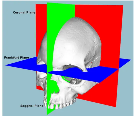
he acquisition process in traditional craniometry does not take in consideration the alignment of the skulls. The anthropologists do not care about the alignment, as they just need to manipulate the skull in a way they can take the measures. To do so, they follow the definition of three planes (based on the three anatomical planes): Saggital, Coronal andFrankfurt (see figure 3.3). These are specifically defined for the craniometry science and have
the following characteristics[29]–[31]:
• Saggital: a vertical plane dividing the skull into 2 symmetrical right and left halves, when viewed from the anterior aspect.
lines.
• Frankfurt: a plane passing through the inferior margin of the left orbit (the point called the left orbitale) and the upper margin of each ear canal or external auditory meatus, a point called the porion.
These three planes are extensively used in the analysis of the skull[32]. From that, and since it is defined as an essential step in manual craniometric studies, it is a natural conclusion that all of the models must be aligned, e.g, placed in the same 3D referencial before any computerized analysis can be made. Normalization of 3D models (alignment) is a common processing stage (pre-processing, actually) in many applications related to computer graphics such as visualization, recognition and shape matching/retrieving. Taking in account its’ importance, a few methods were developed by other authors (explained in further sections). Before focusing on the most relevant methods, it is important to define what is the alignment: a concatenation of isometries (rigid body transform) in 3D space that are used to determine the canonical coordinate system. Usually the center of gravity is chosen and compared to the origin (the origin assures translation invariance). The distinction between two different types of alignment should also be clarified:
1. best alignment between two 3D models;
2. computation of a global coordinate system to all of the models to work with, i.e. have the same coordinate system.
The last, computation of a common coordinate system, is the one of interest in this work. Before going into more detail about the alignment process it is of great importance to distinguish between three types of alignment:
1. Manual - as the name suggests, the alignment is totally manual. The user must specify a set of points to define the three anatomical planes in order to be possible the com-putation of the 3D transformation and consequently transform the 3D position of the model to a pre-defined global coordinate system.
2. Semi Automatic - it means that, from the user perspective, she/he is freed of the picking a set of points task. The interaction is reduced to the minimum possible and the advantages are considerable: less work for the user and, as well, better repeatability, accuracy and ease to use.
3. Automatic - fully automatic alignment. The user has no need of intervention in the process. This could be the ideal and, also, a task of most difficulty to accomplish.
3.3.2 Manual Alignment
T
his approach is simple and easy to develop. The user is responsible to provide (pick) a set of landmark points to be used in the alignment axis and, consequently, compute a 3D transformation to be used in the alignment process.In collaboration with the anthropologists, a set of 7 points were established to be used in the definition of the three alignment axis. The number 7 came as being the minimum number of points needed since a plane can be defined by 3 points or by a point and a normal vector. Two planes were defined with 3 points each and one plane was defined with the remaining point an a vector perpendicular to both previously defined planes. The setting was:
1. Saggital plane - defined with the basion, nasion and bregma points. 2. Frankfurt plane - defined with the orbitale and both left and right porions
3. Coronal plane - defined with the union point and a vector perpendicular to both Sag-gital and Frankfurt planes (cross product between both).
Figure 3.3: The craniometric planes
After defining the three planes, the transformation could be calculated and the model aligned. The alignment, as expected, was correctly made and this approach was maintained as the
solution for manual alignment. The biggest disadvantages of this method are directly corre-lated to the user: the poor repeatability (since the alignment hugely, depends on the user) and a considerable effort to pick all the 7 points.
3.3.3 Automatic Alignment
B
ased on a literature review, it was concluded that the most well-known approach for computing the alignment of 3D objects automatically is based on the PrincipalCom-ponent Analysis (PCA) [33]–[37]. The method is a mathematical procedure that uses an
orthogonal transformation to convert a set of values belonging to a possible set of correlated variables into a set of uncorrelated variables. These are designated as principal components and the number of computed componentes is less or equal to the number of original variables. As the result, the first component has the highest variance and, each of the remaining calcu-lated componentes, in turn, have the highest variance possible under the constraint that they will be ortogonal with the preceding ones. That assures the uncorrelation of the components. Specifically in this case, the method is based on the computation of moments of 3D mod-els[38]. After a translation of the center of mass to the origin of the coordinate system, three principal axes computed with PCA are used to determine the orientation. The experiences presented by the authors just cited show that PCA alignment has two disadvantages:
• It is often imprecise and can produce poor alignments;
• The principal axes are not always good at aligning orientations of different models within the same semantic class.
Podolak et al[39] introduced a planar reflective symmetry transform (PRST) that com-putes a measure of the reflectional symmetry of a 3D shape with respect to all possible planes. They use it to define two new concepts for the global coordinate system: the center of symmetry and the principal symmetry axes. Principal symmetry axes are the normals of the orthogonal set of planes with maximal symmetry, and the center of symmetry is the intersection of those three planes. This approach has been improved by Rustamov with the augmented symmetry transform [40]. Other methods finding symmetries in 3D models have been presented. Minovic et al[41] computed symmetries of a 3D object represented by an octree. Their method is based on the computation of a principal octree aligned with the principal axes. Then they compute a measure of symmetry, the symmetry degree, reasoning with the number of distinct eigenvalues associated to the principal axes. Sun and Sherrah [42] converted the symmetry detection problem to the correlation of the Gaussian image. Then rotational and reflectional symmetry directions are determined using the statistics of the orientation histogram.
An interesting method was developed by Chaouch and Verroust-Blondet. First they make a discrete detection of plane reflection symmetries and classify a model in terms of its symmetry group and the number of its mirror planes. This classification is used to select the good alignment axes among those found by the principal components analysis. Then they introduce local translational invariance cost (LTIC) that measures the invariance of a model with respect to local translation along a given direction. This measure is used to compute the remaining alignment axes when the model has at most one good alignment axis given by the PCA [17].
Another interesting method was developed by Cheng, Leow and Lim[18]. They have focused their work in the alignment of 3D Models of skulls and tried to automatically identify the Frankfurt and Saggital planes. Their approach consisted in the registration of a template skull model with known landmarks to a target skull to locate the landmarks (the two planes) on the target skull. Then, it iteratively refines the landmark locations according to their medical definition.
PCA
A
n experiment was made in order to find out if the PCA could be of good use in the alignment process. The output was a set of 3D axes that were further used to calculate a 3D transformation to align the corresponding model.Figures 3.4, 3.5 and 3.6 show the Scatter plots for the variables of the original coordinates of the 3D model. Worth of mention is the meaning of the variables A, B and C : A corresponds to the X variable, B to the Y variable and C to the Z variable, in euclidean space. Figure 3.4 shows the comparison between the A and B variables, i.e. the correspondent representation of the XY axis in 3D space. The comparison shown by figures 3.5 and 3.6 depicts the representation of the XZ and YZ planes, respectively.
Figure 3.4: Scatterplot for the original coordinates -variables A and B
Figure 3.5: Scatterplot for the original coordinates -variables A and C
Figure 3.6: Scatterplot for the original coordinates -variables B and C
After the PCA was applied the results depicted by the figures 3.7, 3.8 and 3.9 were obtained. The three factors corresponds to the directions of the three axis expected as output (that will further be used to compute the transformation to apply on the model). Figure 3.8 depicts the eigenvectors of the correlation matrix and 3.9 the values of the factors to use in the aforementioned computation of the transformation.
Figure 3.7: Eigenvalues of the correlation matrix (ac-tive variables only)
Figure 3.8: Eigenvectors of the correlation matrix (ac-tive variables only)
Figure 3.9: Factor co-ordinates of the variables (based on correlations)
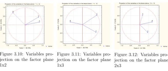
By the analysis of the PCA output it is possible, and useful, to analyse the variables projection on the three different factor-planes. Figures 3.10, 3.11 and 3.12 show that comparison.
Figure 3.10: Variables pro-jection on the factor plane 1x2
Figure 3.11: Variables pro-jection on the factor plane 1x3
Figure 3.12: Variables pro-jection on the factor plane 2x3
At this point it was not possible to make a statement about the success or failure of the method and the next step implied the computation/application of the 3D transformation. Direct observation has shown that the method, only per si, was not enough to make a good alignment, which confirms other authors previously cited. Due to the complexity of the methods implemented by some authors and no guarantee of good alignment in our case, a semi-automatic approach based on a reference skull was investigated.
3.3.4 Semi-automatic Alignment
T
heso called semi-automatic alignment should be considered as an intermediate method to make the alignment of the skull models. The objective was to make acompro-mise between the advantages and disadvantages of both manual and automatic approaches. Iteractive Closest Points (ICP) [43] was the chosen approach.
ICP - Iteractive Closest Points
I
cpis an algorithm developed with the objective of minimizing/registering the diference be-tween two point clouds. The implementation is conceptually simple: interactively revises the transformation needed to minimize the distance between both point clouds.The algorithm workflow is:
• Associate points according to a nearest neighbor criteria;
• Estimate transformation parameters using a mean square cost function; • Transform the points using the estimated parameters;
• Iterate until some criteria is met.
VTK, as the version 5.x, provides an implementation of the algorithm and, naturally, was used as a means to make a semi-automatic alignment.
It is now clear that two point clouds are needed as an input to the algorithm. One is the model that should be aligned; The other was defined as being a template model and could be obtained as the result of a manually aligned skull. It can be argued that the manual alignment could introduce some undesired error but, as shown in the results section, the measures obtained with the use of the so-called template model are conformable with the measures obtained with the manual alignment and, on the other hand, with the traditional method used by the anthropologists. The possible way was to start with only a few models (in the worst case only one), make the manual alignment, and save it as a template model to further use in the alignment with ICP. Following that procedure, it could be possible to make a database of template models and use the more appropriate (in terms of geometric characteristics) for the calculation of the transformation. Currently, only a simple version of the idea was implemented: the user may choose the template model but none is stored in a database and, consequently, the best match is used. It may be a step to take into account in future developments.
From the user perspective, the work flow is:
1. The user selects a model to use as template (Figure 3.13);
2. The template model is displayed as a mean of comparison between both skulls (Figure 3.14). An interaction phase is possible; the model to be aligned can be rotated in all 3 axes (angle in steps of ±2.5 degrees ) in order to get a good first approximation of the alignment, to compute with the ICP algorithm;
3. ICP is applied and the 3D space transformed skull (only) is shown (Figure 3.15). Observation has shown two possible outcomes:
a) Accurate and useful alignment;
b) Completely inaccurate alignment (Figure 3.18). There is no use of the result and the alignment process must be restarted. The user must rotate the model to be aligned in a way that has a relative position (rotation) close to the template model.
Figure 3.13: Unaligned model
Figure 3.14: Model to align and template model (blue)
Figure 3.15: Model aligned - ICP was successful
Figures 3.13, 3.14 and 3.15 shows the case of a successful alignment. On the other hand, figure 3.18 shows the opposite case. The computed affine transformation by ICP cannot be used to fulfil the alignment requirements. The case is depicted in the figures 3.16 to 3.18.
Figure 3.16: Unaligned model
Figure 3.17: Model to align and template model (blue)
Figure 3.18: Model aligned - ICP algorithm has failed
With the ICP implementation the models could now be aligned in a way that is little influenced by the user interaction and, possibly, guarantees acceptable repeatability.
3.3.5 Discussion
A
very considerable amount of effort was made in order to implement/develop the bestmethod to align the models accordingly to the established requirements:• Correspondence to the defined as three planes by the anthropologists team;
• Robust method, capable of assure repeatability of the results (alignment and conse-quent landmark points and measures);
• Easy to use.
The manual alignment gets the job done but, as previously mentioned, has some draw-backs if there is the need of using it often. Repeatability problems could easily arise and the accuracy/veracity of the obtained measures compromised.
A fully automatic approach, as mentioned by some authors and concluded from the attempt described earlier in the text, is difficult to implement and there is no guarantee of correct alignments. After some research on the topic, it was decided to follow a semi automatic approach and ICP was the answer. However, the results have shown one of two situations can occur, as the alignment result:
1. Correct alignment;
2. A result far from the desired alignment, i.e. the model is completely unaligned. It is an important result as the user can easily identify when the algorithm does not produce the desired results and then take the appropriate actions (i.e. refine the position of the model to align by means of rotation of the three axis, X, Y and Z). The fact that ICP works with template models can be also used to make a database of template models and, when the process of choosing the template model, choose the most appropriate from the database instead of requiring the user to choose it. This idea was not implemented in this work but is a strong possibility to be implemented in case of future work.
With the two types of alignment available, the next step was the definition of a set of (initial) points to find. This topic, along with the obtained measures from those defined points, is discussed in detail on the next chapter.
3.4 Methods - Neighbouring and Area Selection
S
incethe first steps on the development that it was clear that having a fully automated system would be too difficult, at least considering the time available to make the disser-tation. The main reason is that several feature points correspond to anatomic structures thatmight be difficult to detect through an algorithm. However, an interactive system where the experts could provide a region of interest (using a pointing device (point & click)) and along a set of rules, defined for each point, could be a good compromise to detect more difficult fea-ture points without the need for precise picking and, at the same time, reducing repeatability problems (the precision would not be dependent of the expert). The same results could be obtained from the (multiple) interaction of different users without compromise the accuracy of the measures. In that perspective, two selection methods were developed:
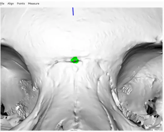
• Neighbouring: the user can specify a neighbourhood by selecting a point. The system will automatically compute the connected n components of the selected point. For example, with n=5 the application will detect and analyse the neighbours in 5 levels of shared vertices. This technique is illustrated in Figure 3.19 to detect the Nasion. The user selects a point close to the point of interest and the neighbouring region (in green) is automatically searched to find the point closest to the YZ plane, i.e. with the minimum X coordinate value.
Figure 3.19: Neighbouring algorithm applied to the nasion
• 3D Box Widget: alternatively, users can also provide a region of interest using a 3D Box Widget to indicate volumes of interest. Figure 3.20 illustrates the use of the technique for the detection of the Glabella. The detected feature point is represented in blue. The area selected by the user, making use of the box widget, is represented in
red. The position of the box widget is initialized in a picked position and can then be moved and resized interactively to define the area of search for the feature.
These two methods (neighbouring and box widget) are available to select any fea-ture point given a simple requirement: the point must be the largest or smallest coor-dinate in one of the 3 axes in the given region. The area of interest can be updated incrementally until the user is satisfied with the resulting detected feature point.
Figure 3.20: Glabella detection using the 3D box widget
Experimentation has shown that the neighbouring method is the most suitable since it provides aproximately the same area of interest as the 3D Box Widget, but is easier to use.
3.4.1 Points
F
romthe application of the aforementioned methods, some landmark points were possible to be obtained. The points can be classified as automatic and semi-automatic, corre-spondingly to the used method.The following points were found automatically (as depicted by figure 3.21):
1. Zygion (bilateral): Given the aligned skull Zygia are defined as the points with maxi-mum and minimaxi-mum X coordinates, respectively to the right and left points. Since the zygomatic arch might not be the largest zone of the skull, it is only consider the portion of the skull with negative Y values;
Figure 3.21: Points automatically found
2. Basion: the point is situated on middle border of the anterior margin of the foramen magnum. This feature point is defined as the point with minimum Y coordinate in the Z axis (considering a threshold of ±0.01 mm in X and ±0.01 mm in Z coordinates); 3. Vertex: Currently this point is not used to compute any measure, but since it is a point
of interest, craniometric wise, and easy to compute we automatically provide it. The point is defined as the highest Y coordinate with the Z and X values within a threshold of ±0.01 mm;
4. Bregma: The algorithm selects a starting point as the coordinate with greater Y value on the region of points of X and Z within a ±0.01 mm threshold. Then, it analyses neighbour points in order to find a discontinuity in the Y values, i.e., sudden smaller followed by higher Y values with the aim of finding the coronal suture. Once the suture region is found, the Bregma is selected as point in the region with smaller Y coordinate. Given its simplicity this measure depends heavily on a correct initial alignment since it does not guarantee to find suture crossing. As future work, further improve the algorithm to avoid such dependence from the alignment should be considered.
5. Opisthocranion: The point is simply defined as the minimal Z coordinate value in the Z plane (sagittal), with X varying within a ±0.01 mm threshold.
Both points were found semi-automatically:
1. Nasion: it’s determined using one of the neighbouring methods. The search is made for the suture, i.e., the point with smallest Z coordinate value. This point is depicted in figure 3.19;
2. Glabella: the neighboring methods search for the coordinate with highest Z coordinate in the selected region. Figure 3.20 illustrates the case.
3.4.2 Measures
T
hemeasures are defined as being the euclidean distance between two points in 3D space. Based on the, initially found, landmark points (see Points), the system was able to provide directly the following relevant craniometric measurements:• Facial width (or Bizygomatic Breath)(ZYB): corresponding to the distance between the two Zygia points;
• Height of the skull (BBH): distance between the Basion and the Bregma points; • Maximum length of the skull (GOL): corresponding to distance between the Glabella
and the Opisthocranion;
• Length of the base of the skull (BNL): corresponding to the distance between the Nasion and the Basion;
• Sagittal frontal arc (FRC): Distance between nasion and bregma;
• Maximum cranial breadth (XCB): From the half-back part of the skull, the distance between the two most lateral points.
Tables 3.1, 3.2 and 3.3 show some measures for three skull models (ids number 25, 38 and 65).
Specialist Neighbour 3D Box 25 user 1 134 136.7 136.7 user 2 136 136.7 136.7 38 user 1 120 121.3 121.3 user 2 119 121.3 121.3 65 user 1 136 136.2 137.2 user 2 134 136.2 136.2
Table 3.1: Facial Width
Specialist Neighbour 3D Box 25 user 1 142 142.6 142.6 user 2 142 142.6 142.6 38 user 1 133 136.8 136.8 user 2 122 136.8 136.8 65 user 1 140 137.8.2 137.8 user 2 139 137.8 137.8
Table 3.2: Height of the skull
Specialist Neighbour 3D Box 25 user 1 106 105.4 105.4 user 2 106 105.4 105.4 38 user 1 95 96.4 96.4 user 2 95 96.4 96.4 65 user 1 105 105.3 105.6 user 2 106 105.6 105.6
Table 3.3: Length of the base of the skull
3.5 Curvature and Normal Analysis
3.5.1 Introduction
W
ith the objective of getting better results, it was decided that methods as Normal analysis and Curvature analysis of the surface of the models could be of great help. As described by [44], the analysis of the curvature can be used in holistic 3D face detection. Salient face features (i.e. regions) such as the eyes and nose were successfully detected on the 3D models used (150 3D faces acquired by an laser range scanner).The idea, and taking in consideration the results obtained by [44] was that, since some regions of interest have an accentuated variation in the surface (e.g. the orbital region), a method could be developed with the aim of facilitating the search of landmark points and
regions of interest to be further analysed.
A tool developed at IEETA, PolyMeCo[45], was used to assert the possible relevance of the Normal and Curvature methodologies, since it makes use of those methodologies for polygonal mesh analysis and comparison, as described in [45]. On the specific case of Poly-MeCo, curvature analysis was also used in segmentatiotn of models (zones of high curvature values were boundaries of the segmented parts from the polydata). Experimentation by vi-sual inspection and discussion with specialist has shown that Normal and Curvature analysis could be useful to detect discontinuities on the mesh, as expeced, but no other conclusion could be obtained relatively to landmark points detection and/or precision improvement on the, already detected, landmark points. At this point was decided to further analyse both methods, described next.
In the three-dimensional space, the Normal to a surface at a point P is a vector that is perpendicular to the tangent plane to that surface at P. The concept of normality generalizes to orthogonality. This concept is often used in computer graphics to determine the surfaces’ orientation toward a light source (for simple light shading) and/or to determine the orien-tation of each vertex toward a light source (for more complex shading, designated as Phong Shading[46]).
In the presented case study the values were computed for each vertex and the process will be described in detail bellow in the text.
The other previously mentioned method, Curvature analysis, it is a widely known method to extract information about the type and amount of curvature of a surface. Before going more deep with the concepts behind the curvature analysis is important to define Principal
Curvatures. Principal Curvatures of a surface at a point are the minimum and maximum
of the normal curvatures at that point (Normal curvatures are the curvatures of curves on the surface lying in planes including the tangent vector at the given point.) The principal curvatures are used to compute the Gaussian and Mean Curvatures of the surface.
• Gaussian curvature: is the product of the principal curvatures at that point; • Mean curvature: is one half the sum of the principal curvatures at that point.
The results from the application of both the curvature types will produce one of the following results:
1. Negative Curvature - the surface is saddle-like (Figure 3.22);
2. Zero Curvature - the surface is flat in, at least, one direction (Figure 3.23); 3. Positive Curvature - the surface is bowl-like (Figure 3.24).
Figure 3.22: Negative Cur-vature
Figure 3.23: Zero (aprox.) Curvature
Figure 3.24: Positive Cur-vature
Illustrations adapted from mcneel.com.
The following two sections will describe the implementation of the Normal and Curvature methods.
3.5.2 Normal Analysis
A
s previously mentioned, Normal componentes were computed for each vertex of the surface. Given a vertex, a search was made in order to find all connected vertices and, with those, the angles between the vertex and all of the connected were summed. At the end of the iteration the summed value was divided by the number of summed values and the result was stored as being the Normal value for the aforementioned point.getAnglesBetweenNormal ( i n p u t mesh ) arrayOfNormalValues : d o u b l e f o r each p o i n t n e i g h b o u r L i s t : a r r a y sumOfNormal : d o u b l e g e t N e i g h b o u r s ( mesh ) : out = n e i g h b o u r L i s t f o r each n e i g h b o u r
item add a n g l e t o sumOfNormal sumOfNormal /= numOfNeighbours
s t o r e v a l u e i n ar ray O fNormal sValue s
Listing 1: Get angle between Normal vectors for a input mesh
Figure 3.25: Curvature analysis - ellip-soidal mesh
Figure 3.26: Normal analysis - ellipsoidal mesh
With simplicity in mind, the first tests were conducted on a ellipsoid mesh. The aim was to automatically detect points of maximum Normal values that correspond to bowl-like region (i.e. the two extreme regions, resembled to the top and bottom of a egg-like shape). Ir order to distinguish between the possible values of the different regions a color map was applied. The results are depicted on figures 3.25 and 3.26. Values in the order of zero were mapped to the red color. The maximum values were mapped to blue. All of the other values in between. A example of the procedure applied to the skull models is depicted in Figure 3.27.
3.5.3 Curvature Analysis
I
n order to find if the analysis of the curvature could provide interesting results, an ex-periment was done. The implementation used was the one provided by VTK. It allows to choose the analysis of four types of curvature: Minimum, Maximum, Gaussian and Mean. Gaussian and Mean curvatures were previously mentioned. Minimum and Maximum curvatures relates to the corresponding value of the Principal Components, i.e. kmin and kmax. kmin= H − p (H2 − K) and kmax = H + p (H2 − K)The exception of spherical and planar surfaces, which have equal principal curvatures, should be considered. For all directions, the curvature will pass through two extrema: a minimum ( kmin) and a maximum ( kmax) which occur at mutually orthogonal directions to
each other.
The curvatures algorithm provided as a part of VTK, only per si, was not enough to reach any conclusion. Thus, an algorithm was created in a way that, given a input mesh (whole model or a part of it), the type of surface to be taken into account (convex or concave), the coordinates of a starting point (e.g. the picked point), and the number of neighbours to consider, it would return a point that best fit to the requirements. In case of more than one point satisfying the requirements, a centroid point would be returned.
The pseudo code is presented next:
getPointMaxCurvature ( i n p u t mesh ) compute c u r v a t u r e s for a i n p u t mesh
f i n d i n i t i a l p o i n t , used t o s t a r t t h e n e i g h b o u r i n g s e a r c h s e a r c h for n n e i g h b o u r s ( c o n n e c t e d v e r t i c e s )
f o r each n e i g h b o u r v e r t e x
g e t and s t o r e c u r v a t u r e v a l u e (map( p o i n t , c u r v a t u r e ) )
if convex
compute for convex shape
e l s e if c on c a v e
compute for c on c a v e shape
if t h e r e i s more than one p o i n t with t h e same c u r v a t u r e
compute t h e c e n t r o i d o f t h o s e p o i n t s
r e t u r n p o i n t
Listing 2: Pseudo code for the algorithm to get the point with maximum curvature, taking into account the neighbours
The direct application of the results provided by the curvatures algorithm, in a ellipsoidal model and using a color pallet to represent the values though colors, has shown quite similar results relatively to the Normal analysis. As a further step, the same procedure was applied using the skull models. Results are depicted in Figure 3.28 for the case of the Mean Curvature and in Figure 3.29 for Gaussian Curvature.
Both methods seem to provide similar results. A question arises: could both methods provide the same results for the analysis? Next section will clarify the question and some conclusions will be described.
The analysis of the results obtained using Normal and Curvature analysis, on the el-lipsoidal and skull models suggest that both methods could be usefull. With that in mind the decision was to go for the Curvature algorithm instead of the Normal algorithm. The justification is based on the following:
• Curvature analysis is provided as part of VTK and consequent there is a guarantee of good integration with the library and available support;
• Its execution times are in the same order of the Normal algorithm (no performance gained).
Figure 3.27: Normal analysis
Figure 3.28: Mean curvature
From this point further, the curvatures algorithm started to be used and it should be considered as the default on the text.
3.5.4 Work Flow
Figure 3.30 depicts the flow diagram of the developed application. Detail about the algorithms behind the menu options will be further explained, through the next chapters.
Figure 3.30: Work flow of the application
3.5.5 User Interface
The interface is composed of 5 menus and a few more sub-menus, as it is shown next:
• File: standard functionality in todays’ applications, such as opening files and terminate the application;
– Open File: shows a open file dialog and, when selected a valid model, loads it; – Exit: terminates the application.
• Align: functionality related to the models alignment;
– Manual: if the user selects the manual alignment then she/he must pick the pre-determined set of points used to compute the alignment;
∗ Pick Points: allows the user to pick a determined number of landmark points; ∗ Align: after the user pick all of the points needed the alignment can be
accomplished using this menu.
– Semi-automatic (ICP): semi-automatic alignment;
∗ Load Template: a loading dialog is shown to allow the user being able to select the template model to use on the alignment via the ICP algorithm; ∗ Align: the alignment is performed.
• Points: functionality related to the determination of the points of interest;
– Try Automatic: the application runs a set of algorithms in order to find the most points possible, in a totally automatic procedure;
– Use Curvature: enables/disables the use of curvature analysis techniques;
– Glabella: semi-automatic point, the user must choose between one of the provided methods;
∗ Neighbouring: the neighbouring algorithm is used;
∗ 3D Box Widget: makes use of the 3D Box Widget algorithm.
– Nasion: semi-automatic point, the user must choose between one of the provided methods. The submenus are the same as the ones available for the Glabella point;
∗ Neighbouring: same as before; ∗ 3D Box Widget: same as before. – Prosthion
∗ Neighbouring: same as before. – Ectomalares
∗ Left;
· Neighbouring: same as before. ∗ Right.
· Neighbouring: same as before. – Biauricular;
∗ Left
· Neighbouring: same as before. ∗ Right
· Neighbouring: same as before. – Nasoespinal;
∗ Neighbouring: same as before. – Frontomallar-Temporalle;
∗ Left;