Performance of tau-lepton reconstruction and identification in CMS

CERN-PH-EP/2011-137 2011/09/29

CMS-TAU-11-001

Performance of τ-lepton reconstruction and identification

in CMS

The CMS Collaboration

Abstract

The performance of τ-lepton reconstruction and identification algorithms is studied using a data sample of proton-proton collisions at√s = 7 TeV, corresponding to an integrated luminosity of 36 pb−1 collected with the CMS detector at the LHC. The τ leptons that decay into one or three charged hadrons, zero or more short-lived neutral hadrons, and a neutrino are identified using final-state particles reconstructed in the CMS tracker and electromagnetic calorimeter. The reconstruction efficiency of the algorithms is measured using τ leptons produced in Z-boson decays. The τ-lepton misidentification rates for jets and electrons are determined.

Submitted to the Journal of Instrumentation

∗_{See Appendix A for the list of collaboration members}

1

Introduction

The primary goal of the Compact Muon Solenoid (CMS) [1] experiment is to explore particle physics at the TeV energy scale by studying the final states produced in the proton-proton collisions at the Large Hadron Collider (LHC) [2]. Leptons play a very important role in these studies because they often represent an experimentally favourable signature.

The three generations of charged leptons, electrons, muons, and taus, are characterized by their masses. Because of their higher mass, τ leptons play a crucial role in the searches for the standard model (SM) Higgs boson, especially for the mass region below twice the W-boson mass. The motivation for searches for the Higgs boson in its τ-leptonic decays is also supported for example by the minimal supersymmetric standard model (MSSM) [3]. Other models of new physics, such as sypersymmetric left-right models (SUSYLR), also predict increased couplings to the third-generation charged fermions. As a result, the decay chains of the supersymmetric particles lead to the lighter stau, which can lead to multi-tau final states [4]. Lepton universality ensures that one third of W and Z-boson leptonic decays result in τ leptons. When measuring rare processes, this contribution becomes substantial. For example, in the search for high-mass SM Higgs bosons that decay preferentially into W and Z bosons, the addition of modes with τ leptons in the final state improves the early discovery potential.

The lifetime of τ leptons is short enough that they decay before reaching the detector ele-ments. In two thirds of the cases, τ leptons decay hadronically, typically into one or three charged mesons (predominantly π+, π−), often accompanied by neutral pions (decaying via π0 → γγ), and a ντ.

The CMS collaboration has designed algorithms that use final-state photons and charged had-rons to identify hadronic decays of τ leptons (τh) through the reconstruction of the intermediate

resonances. The ντ escapes undetected and is not considered in the τh reconstruction. These

algorithms use decay mode identification techniques and efficiently discriminate against po-tentially large backgrounds from quarks and gluons that occasionally hadronize into jets of low particle multiplicity. The algorithms described here have already been successfully used in a measurement of the Z→ττproduction cross section [5] and in a search for neutral MSSM Higgs bosons decaying into τ pairs [6].

This paper describes performance studies based on a sample of proton-proton collisions col-lected during 2010 at√s = 7 TeV, corresponding to an integrated luminosity of 36 pb−1. The analysis uses genuine taus from inclusive Z → ττ production. One tau is required to de-cay leptonically, into a muon, and the other one hadronically, thus creating a µτh final state.

The analysis provides estimates of the τh reconstruction and identification efficiency, and

de-termines the misidentification rate, the probability for quark and gluon jets or electrons to be misidentified as τ_h. This paper uses the selection requirements that are most commonly used in the Z and Higgs analyses, and compares the LHC collision data with predictions based on Monte Carlo (MC) simulation.

2

CMS Detector

A detailed description of CMS can be found elsewhere [1]. The central feature of the CMS apparatus is a superconducting solenoid of 6 m internal diameter, providing a magnetic field of 3.8 T. Within the field volume are the silicon pixel and strip tracker, the crystal electromagnetic calorimeter (ECAL), and the brass/scintillator hadron calorimeter. Muons are measured in gas-ionization detectors embedded in the steel return yoke.

2 3 CMS τhReconstruction Algorithms

CMS uses a right-handed coordinate system, with the origin at the nominal interaction point, the x axis pointing to the centre of the LHC ring, the y axis pointing up perpendicular to the LHC plane, and the z axis along the counterclockwise beam direction. The polar angle θ is measured from the positive z axis and the azimuthal angle φ is measured in the x-y plane. Variables used in this article are the pseudorapidity, η ≡ −ln[tan(θ/2)], and the transverse momentum, pT=

q p2

x+p2y.

The ECAL is designed to have both excellent energy resolution and high granularity, prop-erties that are crucial for reconstructing electrons and photons produced in τ-lepton decays. The ECAL is constructed with projective lead tungstate crystals in two pseudorapidity re-gions: the barrel (|η| < 1.479) and the endcap (1.479 < |η| < 3). In the barrel region, the crystals are 25.8X0 long, where X0 is the radiation length, and provide a granularity of

∆η×∆φ = 0.0174×0.0174. The endcap region is instrumented with a lead/silicon-strip preshower detector consisting of two orthogonal strip detectors with a strip pitch of 1.9 mm. One plane is at a depth of 2X0 and the other at 3X0. The ECAL has an energy resolution of

better than 0.5% for unconverted photons with transverse energies above 100 GeV.

The inner tracker measures charged particle tracks within the range|η| < 2.5. It consists of 1 440 silicon pixel and 15 148 silicon strip detector modules, and provides an impact parameter resolution of∼15 µm and a transverse momentum resolution of about 1.5% for 100 GeV par-ticles. The reconstructed tracks are used to measure the location of interaction vertex(es). The spatial resolution of the reconstruction is ≈ 25µm for vertexes with more than 30 associated tracks [7].

The muon barrel region is covered by drift tubes, and the endcap regions by cathode strip chambers. In both regions, resistive plate chambers provide additional coordinate and timing information. Muons can be reconstructed in the range|η| <2.4, with a typical p_Tresolution of 1% for pT ≈40 GeV/c.

3

CMS τ

Reconstruction Algorithms

CMS has developed two algorithms for identifying τ_h decays, based on the categorization of the τ_h-decay channels through the reconstruction of intermediate resonances: the hadron plus strips (HPS) and the tau neural classifier (TaNC) algorithms. The HPS algorithm is used as the main algorithm in most previous CMS τ analyses, with TaNC used for crosschecks. Both algorithms use particle flow (PF [8]) particles. In the PF approach, information from all sub-detectors is combined to reconstruct and identify all particles produced in the collision. The particles are classified into mutually exclusive categories: charged hadrons, photons, neutral hadrons, muons, and electrons. These algorithms are designed to optimize the performance of the τ_h identification and reconstruction by considering the different hadronic decay modes of the tau individually. The dominant hadronic decays of τ leptons consist of one or three charged πmesons and up to two π0mesons, as summarized in Table 1.

Both algorithms start the reconstruction of a τhcandidate from a PF jet, whose four-momentum

is reconstructed using the anti-kT algorithm with a distance parameter R = 0.5 [10]. Using a

PF jet as an initial seed, the algorithms first reconstruct the π0 components of the τh, then

combine them with charged hadrons to reconstruct the tau decay mode and calculate the tau four-momentum and isolation quantities.

Table 1: Branching fractions of the dominant hadronic decays of the τ lepton and the sym-bol and mass of any intermediate resonance [9]. The h stands for both π and K, but in this analysis the π mass is assigned to all charged particles. The table is symmetric under charge conjugation.

Decay mode Resonance Mass (MeV/c2) Branching fraction (%)

τ−→h−ντ 11.6% τ−→h−π0ντ ρ− 770 26.0% τ−→h−π0π0ντ a − 1 1200 9.5% τ−→h−h+h−ντ a−₁ 1200 9.8% τ−→h−h+h−π0ντ 4.8% 3.1 HPS Algorithm

The HPS algorithm gives special attention to photon conversions in the CMS tracker material. The bending of electron/positron tracks in the magnetic field of the CMS solenoid broadens the calorimeter signatures of neutral pions in the azimuthal direction. This effect is taken into account in the HPS algorithm by reconstructing photons in “strips”, objects that are built out of electromagnetic particles (PF photons and electrons). The strip reconstruction starts by center-ing a strip on the most energetic electromagnetic particle within the PF jet. The algorithm then searches for other electromagnetic particles within a window of size∆η = 0.05 and∆φ= 0.20 centered on the strip center. If other electromagnetic particles are found within that window, the most energetic one gets associated with the strip and the strip four-momentum is recalcu-lated. The procedure is repeated until no further particles are found that can be associated with the strip. Strips satisfying a minimum transverse momentum requirement of pstrip_T > 1 GeV/c are finally combined with the charged hadrons to reconstruct individual τhdecay modes.

The decay topologies that are considered by the HPS tau identification algorithm are

1. Single hadron corresponds to h−ντand h−π0ντ decays in which the neutral pions have too little energy to be reconstructed as strips.

2. One hadron+one strip reconstructs the decay mode h−π0ντin events in which the photons from π0decay are close together on the calorimeter surface.

3. One hadron+two strips corresponds to the decay mode h−π0ντin events in which photons from π0_{decays are well separated.}

4. Three hadrons corresponds to the decay mode h−h+h−ντ. The three charged hadrons are required to come from the same secondary vertex.

There are no separate decay topologies for the h−π0π0 and h−h+h−π0ντ decay modes. They are reconstructed via the existing topologies. All charged hadrons and strips are required to be contained within a cone of size ∆R = (2.8 GeV/c)/pτh

T, where p

τh

T is the transverse

mo-mentum of the reconstructed τh. The reconstructed tau momentum~pτh is required to match

the (η, φ) direction of the original PF jet within a maximum distance of ∆R = 0.1, where ∆R=p(∆η)2_{+ (∆φ)}2_.

The four-momenta of charged hadrons and strips are reconstructed according to the respective τh decay topology hypothesis, assuming all charged hadrons to be pions, and are required

to be consistent with the masses of the intermediate meson resonances listed in Table 1. The following invariant mass windows are allowed for candidates: 50 – 200 MeV/c2 for π0, 0.3 –

4 3 CMS τhReconstruction Algorithms

1.3 GeV/c2for ρ, and 0.8 – 1.5 GeV/c2for a1. In cases where a τh decay is consistent with more

than one hypothesis, the hypothesis giving the highest pτh

T is chosen.

Finally, reconstructed candidates are required to be isolated. The isolation criterion requires that, apart from the τhdecay products, there be no charged hadrons or photons present within

an isolation cone of size∆R=0.5 around the direction of the τh. By adjusting the pTthreshold

for particles that are considered in the isolation cone, three working points, ”loose”, ”medium”, and ”tight” are defined. The working points are determined using a simulated sample of QCD dijet events. The “loose” working point corresponds to a probability of approximately 1% for jets to be misidentified as τh. Successive working points reduce the misidentification rate by a

factor of two with respect to the previous one.

3.2 TaNC Algorithm

In the TaNC case the leading (highest-pT) particle is required to have a pT above 5 GeV/c and

to be within∆R=0.1 around the jet direction. The PF τhfour-momentum is reconstructed as a

sum of the four-momenta of all particles with pTabove 0.5 GeV/c in a cone of radius∆R=0.15

around the direction of the leading particle. A signal cone size is defined to be ∆Rphotons =

0.15 for photons and∆Rcharged = (5 GeV)/ET for charged hadrons, where ETis the transverse

energy of the PF τh, and∆Rcharged is restricted to be within the range 0.07≤ ∆Rcharged ≤ 0.15.

The signal cone is the region where the τhdecay products are expected to be found. An isolation

annulus is defined between the signal cone and a wider isolation cone of outer radius∆R=0.5 around the leading particle.

The decay mode is reconstructed from the particles that are contained within the signal cone of the τhcandidate by counting the number of tracks and π0meson candidates. The π0meson

candidates are reconstructed by merging pairs of photons that have an invariant mass of less than 0.2 GeV/c2. All unpaired photons are considered as π0candidates if their pT exceeds 10%

of the PF τhtransverse momentum.

The decay mode of each τh candidate is uniquely determined by the multiplicity of

recon-structed objects in the signal cone. Candidates with decay topologies other than those listed in Table 1 are immediately rejected. Otherwise, a neural network is used to compute a discrimi-nant quantity for the τhcandidate. Each decay mode of Table 1 uses a different neural network.

The input observables used for each neural network are optimized for the topology of the decay mode, and are constructed from the four-momenta of the particles in the signal cone and the isolation annulus. In general, the signal cone input observables are chosen to parameterize the decay kinematics of the intermediate resonance, and the isolation cone observables to describe the multiplicity and pT spectrum of nearby particles. The variables include angular

correla-tions between different particles within the signal and the isolation cones, invariant masses calculated using different combinations of the particles, transverse momenta, and numbers of charged particles in the signal and the isolation regions. The neural networks are trained to discriminate between genuine τh produced in Z → ττ decays and misidentified jets from a sample of QCD multijet events. The set of input observables for a given neural network is chosen to be the minimal set of observables for which the removal of any two input variables significantly degrades the classification performance.

The output of the neural network is a continuous quantity. By adjusting the thresholds of selections on the neural network output, three working points, again called “loose”, “medium”, and “tight”, are defined, similar to those discussed in Section 3.1.

4

Efficiency of τ

Reconstruction and Identification

To compare the performance of τhreconstruction in data and MC simulation, a set of MC

sam-ples is used to reproduce a mixture of signal and background events. The signal is expected to come from inclusive Z → ττproduction. The major sources of background are ττ Drell–Yan production outside of the Z-mass region, W production with associated jets, QCD multijet, and t¯t production. The Drell–Yan signal and background are simulated with the next-to-leading order (NLO) MC generator POWHEG [11–13]. The QCD multijet and W backgrounds are sim-ulated with PYTHIA [14] and the top quark samples with Madgraph [15]. The τ-lepton decays are simulated with Tauola [16]. The samples are normalized using the cross section at next-to-next-to-leading order (NNLO) for Drell–Yan and W, at leading order (LO) for QCD, and NLO for the t¯t sample. The MC samples are mixed based on the corresponding cross sections. To measure the efficiency of τhreconstruction and identification in data, a tag-and-probe method

is used with a sample of Z → ττ → µτh events. The events are preselected using kinematic

cuts and a set of requirements to suppress the background from Z→ µµ, W, and QCD events, but without applying the τ_h-identification algorithms. The preselection requires the event to be triggered by a single-muon high level trigger [17], and to contain only one isolated muon with pµ_T > 15 GeV/c within the geometric acceptance η_µ

 < 2.1, that is used as a tag. An isolated jet candidate of pjet_T > 20 GeV/c within the geometric acceptance η_jet

 < 2.3, with a “leading” (highest-pT) track constituent in the jet with pT > 5 GeV/c, is used as a probe. The

preselection is needed to increase the percentage of Z → ττ events in the final sample. This preselection clearly biases the sample, but the bias is taken into account when computing the final efficiency. The four-momentum of the jet is reconstructed using the anti-kTalgorithm with

a distance parameter of 0.5 [10]. The muon and the “leading” track in the jet are required to be of opposite charge. To suppress background from W+jet(s) events, an additional requirement on transverse mass, MT, of the muon and missing transverse energy, ETmiss, of less than 40 GeV

is applied. The transverse mass is defined as MT =

q

2p_TµEmiss

T · (1−cos∆φ), where p

µ

T is the

muon transverse momentum and∆φ is the azimuthal angle between the Emiss_T vector and pµ_T. The HPS and TaNC algorithms are both applied to the preselected events. The resulting invari-ant mass distributions of the µ-jet system for those events that pass or fail the τ_hidentification are fitted using signal and background distributions provided by MC simulation. The effi-ciency is then calculated as ε = NZ→ττ

pass /(NpassZ→ττ+NfailZ→ττ), where Npass,failZ→ττ are the numbers of

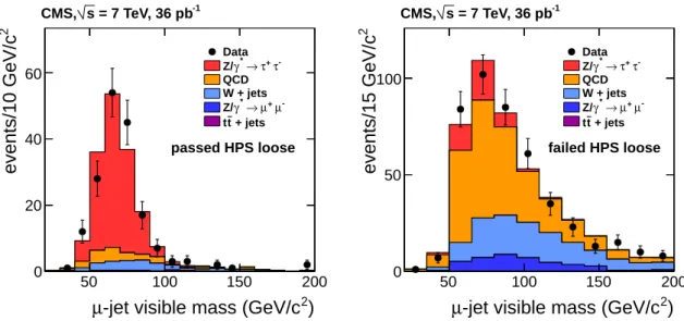
Z → ττ events after background contributions are subtracted. Figure 1 shows the invariant mass of the µ-jet system for preselected events that pass (left) and fail (right) the “loose” τh

identification requirements. Since in the “failed” sample there is no τhreconstructed, for

con-sistency the visible mass is always computed using the jet four-vector and not the four-vector as reconstructed by the τ_halgorithms. The MC predictions for signal and background events are also shown. The “passed” sample is dominated by Z events and a small background con-tribution. The sample of “failed” events is dominated by background contributions. The MC predictions describe the data reasonably well. The stability of the fit results is tested by using background estimates from data instead of the MC predictions and by varying the invariant mass ranges for the fit. All checks demonstrate consistent results within the uncertainties of the method.

Results of the fits are summarized in Table 2. The values measured in data, “Fit data”, are com-pared with the expected values, “Expected MC”, obtained by repeating the fitting procedure on simulated events. The efficiency of the τhalgorithms on preselected events is approximately

ef-6 4 Efficiency of τhReconstruction and Identification

)

2

-jet visible mass (GeV/c

µ 50 100 150 200 2 events/10 GeV/c 0 20 40 60 Data -τ + τ → * γ Z/ QCD W + jets -µ + µ → * γ Z/ + jets t t -1 = 7 TeV, 36 pb s CMS, passed HPS loose ) 2

-jet visible mass (GeV/c

µ 50 100 150 200 2 events/15 GeV/c 0 50 100 Data -τ + τ → * γ Z/ QCD W + jets -µ + µ → * γ Z/ + jets t t -1 = 7 TeV, 36 pb s CMS, failed HPS loose

Figure 1: Invariant mass distribution of the µ-jet system for preselected events which pass (left) and fail (right) the HPS “loose” τ_h identification requirements (solid symbols) compared to predictions of the MC simulation (histograms).

Table 2: Efficiency for a τhto pass the HPS and TaNC identification criteria, measured by fitting

the Z→ττsignal contribution in the samples of the “passed” and “failed” preselected events. The uncertainties of the fit are statistical only. The statistical uncertainties of the MC predictions are small and can be neglected. The last column represents the data-to-MC correction factors and their full uncertainties including statistical and systematic components. Data-to-MC ratios for the τh reconstruction efficiency determined using fits to the measured Z production cross

sections as described in [5] are also shown.

Algorithm Fit data Expected MC Data/MC HPS “loose” 0.70±0.15 0.70 1.00±0.24 HPS “medium” 0.53±0.13 0.53 1.01±0.26 HPS “tight” 0.33±0.08 0.36 0.93±0.25 TaNC “loose” 0.76±0.20 0.72 1.06±0.30 TaNC “medium” 0.63±0.17 0.66 0.96±0.27 TaNC “tight” 0.55±0.15 0.55 1.00±0.28 HPS “loose” ττcombined fit [5] 0.94±0.09

ficiency depends on the pT and η requirements, which are applied in each individual physics

analysis. The main goal of this study is to perform the data-to-MC comparison and to deter-mine data-to-MC correction factors and their uncertainties. The agreement in the mean values of the fits between data and MC simulation is observed to be better than a few percent, although with this data sample, the statistical uncertainties of the fits are in the range of 20–30%.

Systematic uncertainties on the measured τh identification efficiencies arise from

uncertain-ties on track reconstruction (4%) and from uncertainuncertain-ties on the probabiliuncertain-ties for jets to pass the “leading” track pT and loose isolation requirements applied in the preselection (≤ 12%).

Uncertainties on track momentum and τh energy scales have an effect on the measured τh

identification efficiencies below 1%. All numbers represent relative uncertainties.

The resulting ratio of the measured efficiencies to those predicted by MC simulation for τh

de-cays to pass the “loose”, “medium”, and “tight” HPS and TaNC working points are presented in the last column of Table 2. The uncertainties on the ratios represent the full uncertainties of the method, which are calculated by adding the statistical and systematic uncertainties in quadrature. The total uncertainty of the measured efficiency of the τhalgorithms is dominated

by the statistical uncertainty of the fit. The simulation describes the data well. Since the same event sample is used to evaluate efficiencies for different working points, the results are corre-lated.

The values presented in Table 2 are used as inputs for fits to measure the uncertainty of the τhreconstruction and identification efficiency with higher precision by comparing the yield of

the Z → ττ events in different decay modes and the yield of Z → µµ and Z → ee events, as described elsewhere [5]. The first approach uses a simultaneous fit of the four Z → ττ decay channels with final states µµ, eµ, µτh, and eτh. As a result of the fit, the combined cross

section and τ_hefficiency are measured. The data-to-MC correction factor for the HPS “loose” working point is measured to be 0.94±0.09. The second approach is based on a comparison of the τh channels, Z → µτh and eτh, to the combined Z → µµ, ee cross section as measured

by CMS. The data-to-MC correction factor for the HPS “loose” working point in this case is measured to be 0.96±0.07. The slightly smaller uncertainty of the latter method is explained by the higher precision of the combined Z→ µµ, ee cross-section measurement. These values are also presented in Table 2. Both approaches yield more precise uncertainties, 9% and 7%, than the 24% from the tag-and-probe method, for the “loose“ HPS working point. To achieve this precision, the methods rely on assumptions about the physics source of the signal, i.e., the values of the inclusive Z production cross section and Z → ττ branching fraction, and the absence of non-SM sources in the data sample. In physics analyses where these assumptions cannot be made, such as the measurement of the Z→ττproduction cross section itself [5] and the search for H →ττ[6], the tag-and-probe method remains the only one available.

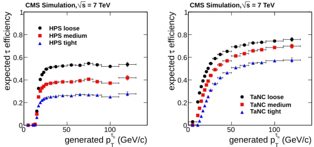
The expected τh efficiency values from the Z → ττ process, with a reconstructed |ητh| < 2.3,

and either pτh

T > 15 GeV/c or p

τh

T > 20 GeV/c, are estimated using simulated events and

pre-sented in Table 3. The selections are applied both at the generated and reconstructed levels. A matching of∆R<0.15 between the generated and reconstructed τ_hdirections is required. Fig-ure 2 shows the expected efficiencies as a function of the generated pτh

T for all working points

of each algorithm.

5

Reconstruction of the τ

Decay Mode

The correlation between the generated and reconstructed τh decay modes is studied using a

8 5 Reconstruction of the τhDecay Mode

Table 3: The expected efficiency for τ_hdecays to pass the HPS and TaNC identification criteria estimated using Z → ττ events from the MC simulation for two different selection require-ments on pτh

T. The requirement is applied both at the reconstruction and generator levels. The

statistical uncertainties of the MC predictions are smaller than the least significant digit of the efficiency values in the table and are not shown.

Algorithm HPS TaNC

“loose” “medium” “tight” “loose” “medium” “tight” Efficiency (pτh T >15 GeV/c) 0.46 0.34 0.23 0.54 0.43 0.30 Efficiency (pτh T >20 GeV/c) 0.50 0.37 0.25 0.58 0.48 0.36 (GeV/c) h τ T generated p 0 50 100 e ff ic ie n c y τ expected 0 0.2 0.4 0.6 0.8 1 HPS loose HPS medium HPS tight = 7 TeV s CMS Simulation, (GeV/c) h τ T generated p 0 50 100 e ff ic ie n c y τ expected 0 0.2 0.4 0.6 0.8 1 TaNC loose TaNC medium TaNC tight = 7 TeV s CMS Simulation,

Figure 2: The expected efficiency of the τhalgorithms as a function of generated pτTh, estimated

using a sample of simulated Z→ττevents for the HPS (left) and TaNC (right) algorithms, for the ”loose”, ”medium”, and ”tight” working points.

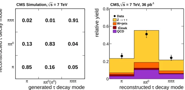
0.85 0.16 0.05 0.13 0.83 0.04 0.02 0.01 0.91 decay mode τ generated π _ππ0_(π0₎ πππ decay mode τ reconstructed π 0 π π π π π = 7 TeV s CMS Simulation, decay mode τ reconstructed π _ππ0 πππ relative yield 0 0.2 0.4 0.6 0.8 Data τ τ → Z W+jets /ewk t t QCD -1 = 7 TeV, 36 pb s CMS,

Figure 3: (left) The fraction of generated τh decays of a given type reconstructed in a certain

decay mode for the HPS “loose” working point from simulated Z → ττ events. (right) The relative yield of τhreconstructed in different decay modes in the Z → ττ → µτh data sample

compared to the MC predictions. The MC simulation is a mixture of the signal and background samples based on the corresponding cross sections, as shown by the histograms.

represents one generated decay mode normalized to unity. Each row corresponds to one recon-structed decay mode. The numbers demonstrate the fraction of generated τh of a given type

reconstructed in a specific decay mode. Both generated and reconstructed τh are required to

have a visible transverse momentum pτh

T >15 GeV/c, and to match within a cone of∆R=0.15.

For each of the generated decay modes, the fraction of correctly reconstructed decays is more than 80%, reaching 90% for the three-charged-pion decay mode.

A data-to-MC comparison of the relative yield of events reconstructed in different τ_h decay modes in a data sample of Z → ττ → µτ_h events is shown in Fig. 3 (right). The events are selected using the requirements described in [5]. The τhcandidates are required to have visible

transverse momenta pτh

T >20 GeV/c within the geometric acceptance|η| <2.3. The MC sample

represents a mixture of the signal and background MC samples based on the corresponding cross sections. The performance of the τhalgorithm is well reproduced by the MC simulation.

6

Reconstruction of the τ

Energy

Since charged hadrons and photons are reconstructed with high precision using the PF tech-niques, the reconstructed τhenergy is expected to be close to the true energy of its visible decay

products. According to simulation, the ratio of the reconstructed to the true visible τh energy

for the HPS algorithm is constant as a function of energy and within 2% of unity, while for TaNC it decreases by about 2% as pτh

T approaches 60 GeV/c. The η dependence is more pronounced.

For both algorithms the reconstructed τh energy is underestimated by 5% with respect to the

true energy as one moves towards higher η (from barrel to endcap region).

The quality of the τhenergy scale simulation can be examined by analyzing the Z→ττ→µτh

data sample. The reconstructed invariant mass of the µτhsystem is very sensitive to the energy

scale of the τh, since the muon four-momenta are measured with high precision. By varying the

10 7 Measurement of the τhMisidentification Rate for Jets ) 2 ) mass (GeV/c 0 π π ( τ visible 0.4 0.6 0.8 1 1.2 1.4 arbitrary units 0 0.2 0.4 0.6 Data Simulation TauES*1.03 TauES*0.97 -1 = 7 TeV, 36 pb s CMS, ) 2 ) mass (GeV/c π π π ( τ visible 0.4 0.6 0.8 1 1.2 1.4 1.6 1.8 arbitrary units 0 0.2 0.4 0.6 Data Simulation TauES*1.03 TauES*0.97 -1 = 7 TeV, 36 pb s CMS,

Figure 4: The reconstructed invariant mass of τh decaying into one charged and one neutral

pion (left) and into three charged pions (right) from data, compared to predictions of the simu-lation. The solid lines represent results of the best fit described in the text and the dashed lines represent the predictions with the tau energy scale, TauES, varied up and down by 3% with respect to the best fit value.

produced. The resulting templates are fitted to the data and the best agreement is achieved by scaling the τh energy in simulation by a factor 0.97±0.03, where the uncertainty is averaged

over the pseudorapidity range of the data sample.

A complementary procedure, which does not assume knowledge of the ττ invariant mass spec-trum, is based on the invariant mass of reconstructed τh constituents, shown in Fig. 4. The

method uses τhas an independent object but relies on good understanding of underlying

back-ground events that contribute to the signal sample. The fit is performed separately for ππ0_and

πππ decay channels, since the major source of the uncertainty is expected to come from re-construction of the electromagnetic energy. The simulation describes both decay channels well. The best agreement is achieved by scaling the τh energy in simulation by a factor 0.97±0.03

for the ππ0 decay mode and by a factor 1.01±0.02 for the πππ decay mode. The effect of the energy-scale uncertainty on the shape of the τhinvariant mass distribution is also shown in

Fig. 4. Varying the energy scale in simulation by the uncertainty derived from the µτhinvariant

mass fit, i.e. 3%, corresponds to a significant deviation in the predicted τhmass shape.

7

Measurement of the τ

Misidentification Rate for Jets

Jets that could be misidentified as τhhave different properties depending on their origin. Most

of the jets are produced in QCD processes, either with or without the associated production of Z or W bosons. To distinguish between them, different data samples are selected. The QCD-type, gluon-enriched, jets are selected using events with at least one jet of transverse momentum pjet_T > 15 GeV/c and a second jet of pjet_T > 10 GeV/c, both within|η| < 2.5. The Z- and W-type, quark-enriched, jets are selected by requiring at least one isolated muon with transverse mo-mentum pT >15 GeV/c and|η| <2.1 and a jet of transverse momentum pjet_T >10 GeV/c within

|η| <2.5. In addition, a muon-enriched QCD sample is selected by requiring a muon and a jet, but suppressing the W contribution by selecting events with MT <40 GeV/c2. For each of these

samples additional selection requirements are applied to suppress the background contribution from events with jets from other sources.

Figure 5 shows the τ_h misidentification rate as a function of the jet pT for the “loose” working

points of the HPS and TaNC algorithms, where the measured values are compared with the MC predictions for the different types of jets. The misidentification rates expected from simulation, and the measured data-to-MC ratios are summarized in Table 4 for the three working points of both reconstruction algorithms. The values are integrated over the pT and η phase space

used in the Z → ττ analysis, pjet_T > 20 GeV/c and |η| < 2.3. The misidentification rate as a function of reconstruction efficiency for all working points of both algorithms is shown in Fig. 6, which summarizes the MC estimated efficiency and the measured misidentification rate values presented in Tables 3 and 4. Since the QCD and µ-enriched QCD misidentification rate values are observed to be similar, only one set of QCD points is shown. Open symbols represent results obtained by running an early fixed-cone τh-identification algorithm, used in the CMS

physics technical design report (PTDR, [18]) on simulated events. The decay-mode-based HPS and TaNC algorithms perform significantly better than the fixed-cone algorithm.

0 50 100 150 200

misidentification rate for jets

τ -3 10 -2 10 Data ν µ → W Simulation ν µ → W QCD Data QCD Simulation Data µ QCD Simulation µ QCD HPS loose -1 = 7 TeV, 36 pb s CMS, (GeV/c) T jet p 0 50 100 150 200 Simulation Data-Sim. -0.2 0 0.2 0 50 100 150 200

misidentification rate for jets

τ -3 10 -2 10 Data ν µ → W Simulation ν µ → W QCD Data QCD Simulation Data µ QCD Simulation µ QCD TaNC loose -1 = 7 TeV, 36 pb s CMS, (GeV/c) T jet p 0 50 100 150 200 Simulation Data-Sim. -0.2 0 0.2

Figure 5: Misidentification probabilities for jets to pass “loose” working points of the HPS (left) and TaNC (right) algorithms as a function of jet pT for QCD, µ-enriched QCD, and W

type events. The misidentification rates measured in data are shown by solid symbols and compared to MC prediction, displayed with open symbols.

8

Measurement of the τ

Misidentification Rate for Electrons

Isolated electrons passing the identification and isolation criteria of the τhalgorithms are also

an important source of background in many analyses with τh in the final state. In this case

the electron is misidentified as a pion originating from τ_h. A multivariate discriminant is used to reduce this background, improving the separation between pions and electrons. The dis-criminant is implemented in the PF algorithm and its output is denoted by ξ. The value of the

12 8 Measurement of the τhMisidentification Rate for Electrons

efficiency

τ

expected

0.1 0.2 0.3 0.4 0.5 0.6

misidentification rate for jets

τ

efficiency

τ

expected

misidentification rate for jets

τ

Figure 6: The measured τh misidentification rate as a function of the MC-estimated τh

re-construction efficiency for the three working points of the HPS and TaNC algorithms from µ-enriched QCD and W data samples. For each algorithm the “loose”, “medium”, and “tight” selections are the points with highest, middle and lowest efficiencies respectively. The PTDR points represent results of the fixed-cone τh-identification algorithm [18] on simulation.

Table 4: The MC predicted τ_h misidentification rates and the measured data-to-MC ratios, in-tegrated over the pTand η phase space typical for the Z→ττanalysis.

Algorithm QCD QCDµ W + jets

MC (%) Data/MC MC (%) Data/MC MC (%) Data/MC HPS “loose” 1.0 1.00±0.04 1.0 1.07±0.01 1.5 0.99±0.04 HPS “medium” 0.4 1.02±0.06 0.4 1.05±0.02 0.6 1.04±0.06 HPS “tight” 0.2 0.94±0.09 0.2 1.06±0.02 0.3 1.08±0.09 TaNC “loose” 2.1 1.05±0.04 1.9 1.12±0.01 3.0 1.02±0.05 TaNC “medium” 1.3 1.05±0.05 0.9 1.08±0.02 1.6 0.98±0.07 TaNC “tight” 0.5 0.98±0.07 0.4 1.06±0.02 0.8 0.95±0.09

discriminant ξ ranges between−1.0 (most compatible with the pion hypothesis) and 1.0 (most compatible with the electron hypothesis).

Two selected working points, corresponding to ξ < −0.1 and ξ < 0.6, are considered in this analysis. The first working point rejects even those electrons, that are poorly reconstructed and is optimized for a low misidentification rate, about 2%, at the price of about 4% losses of genuine τh. The second working point suffers from larger misidentification rates of about

20%, since it was optimized for τh efficiencies exceeding 99.5%. It rejects only well identified

electrons.

The probability for an electron to be misidentified as τ_h, the e → τ_h misidentification rate, is determined using a sample of isolated electrons coming from the decay Z → ee. The events are required to have a reconstructed electron and an electron that is reconstructed as τh. The

particles must have opposite charge. The invariant mass of the pair is required to be between 60 and 120 GeV/c2. The tag electron is required to be isolated and to have a pT in excess of

25 GeV/c. The second electron, a probe, is required to pass the HPS “loose” working point, without requiring any specific veto against electrons, and have pT in excess of 15 GeV/c. The

e →τhmisidentification rate is estimated by measuring the ratio between the number of probes

passing the electron-rejection discriminant and the overall number of selected probes. The sample of events that does not pass the electron-rejection discriminant, is populated by well-reconstructed electrons. The sample that passes the discriminant contains poorly well-reconstructed electrons, as well as other background contributions, “misidentified electrons“. To remove the contamination from misidentified electrons, a background subtraction procedure is performed by fitting the passing and failing eτhinvariant mass distributions to the superposition of signal

and background components.

Table 5 gives the ratio between the misidentification rates as measured in the data and those obtained using MC simulation for two|η|bins. In the central η region, the simulation underes-timates the measured misidentification rates. Within the uncertainties of the measurement the data-to-MC ratios for both discriminants agree in the same η intervals.

Table 5: The e→τhmisidentification rates, found by applying the tag-and-probe method to the

MC simulation and the ratio of the tag-and-probe values obtained in data and MC simulation, shown in two regions of η and for two working points of the electron-rejection discriminant.

Bin Discriminant ξ < −0.1 Discriminant ξ <0.6

|η| MC (%) Data/MC MC (%) Data/MC

<1.5 2.21±0.05 1.13±0.17 13.10±0.08 1.14±0.04 >1.5 3.96±0.09 0.82±0.18 26.80±0.16 0.90±0.04

9

Summary

The performances of two reconstruction algorithms for hadronic tau decays developed by CMS, HPS and TaNC, have been studied using the data sample collected at a centre-of-mass energy of 7 TeV in 2010 and corresponding to an integrated luminosity of 36 pb−1. Both al-gorithms show good performance in terms of τh identification efficiency, approximately 50%,

while keeping the misidentification rate for jets at the level of∼1%. The MC simulation was found to describe the data well. The τ_hidentification efficiency was measured with an uncer-tainty of 24% by using a tag-and-probe method in a Z→ ττ → µτ_h data sample, and with an uncertainty of 7% by using a global fit to all Z→ττdecay channels and constraining the yield to the measured combined Z→ µµ, ee cross section. The scale factor for measured τ_henergies was found to be close to unity with a relative uncertainty less than 3%.

14 9 Summary

Acknowledgments

We wish to congratulate our colleagues in the CERN accelerator departments for the excellent performance of the LHC machine. We thank the technical and administrative staff at CERN and other CMS institutes. This work was supported by the Austrian Federal Ministry of Science and Research; the Belgium Fonds de la Recherche Scientifique, and Fonds voor Wetenschappelijk Onderzoek; the Brazilian Funding Agencies (CNPq, CAPES, FAPERJ, and FAPESP); the Bul-garian Ministry of Education and Science; CERN; the Chinese Academy of Sciences, Ministry of Science and Technology, and National Natural Science Foundation of China; the Colom-bian Funding Agency (COLCIENCIAS); the Croatian Ministry of Science, Education and Sport; the Research Promotion Foundation, Cyprus; the Estonian Academy of Sciences and NICPB; the Academy of Finland, Finnish Ministry of Education and Culture, and Helsinki Institute of Physics; the Institut National de Physique Nucl´eaire et de Physique des Particules / CNRS, and Commissariat `a l’ ´Energie Atomique et aux ´Energies Alternatives / CEA, France; the Bundes-ministerium f ¨ur Bildung und Forschung, Deutsche Forschungsgemeinschaft, and Helmholtz-Gemeinschaft Deutscher Forschungszentren, Germany; the General Secretariat for Research and Technology, Greece; the National Scientific Research Foundation, and National Office for Research and Technology, Hungary; the Department of Atomic Energy and the Department of Science and Technology, India; the Institute for Studies in Theoretical Physics and Mathe-matics, Iran; the Science Foundation, Ireland; the Istituto Nazionale di Fisica Nucleare, Italy; the Korean Ministry of Education, Science and Technology and the World Class University program of NRF, Korea; the Lithuanian Academy of Sciences; the Mexican Funding Agencies (CINVESTAV, CONACYT, SEP, and UASLP-FAI); the Ministry of Science and Innovation, New Zealand; the Pakistan Atomic Energy Commission; the State Commission for Scientific Re-search, Poland; the Fundac¸˜ao para a Ciˆencia e a Tecnologia, Portugal; JINR (Armenia, Belarus, Georgia, Ukraine, Uzbekistan); the Ministry of Science and Technologies of the Russian Feder-ation, the Russian Ministry of Atomic Energy and the Russian Foundation for Basic Research; the Ministry of Science and Technological Development of Serbia; the Ministerio de Ciencia e Innovaci ´on, and Programa Consolider-Ingenio 2010, Spain; the Swiss Funding Agencies (ETH Board, ETH Zurich, PSI, SNF, UniZH, Canton Zurich, and SER); the National Science Council, Taipei; the Scientific and Technical Research Council of Turkey, and Turkish Atomic Energy Authority; the Science and Technology Facilities Council, UK; the US Department of Energy, and the US National Science Foundation.

Individuals have received support from the Marie-Curie programme and the European Re-search Council (European Union); the Leventis Foundation; the A. P. Sloan Foundation; the Alexander von Humboldt Foundation; the Belgian Federal Science Policy Office; the Fonds pour la Formation `a la Recherche dans l’Industrie et dans l’Agriculture (FRIA-Belgium); the Agentschap voor Innovatie door Wetenschap en Technologie (IWT-Belgium); and the Council of Science and Industrial Research, India.

References

[1] CMS Collaboration, “The CMS experiment at the CERN LHC”, JINST 03 (2008) S08004. doi:10.1088/1748-0221/3/08/S08004.

[2] L. Evans and P. Bryant, “LHC Machine”, JINST 03 (2008) S08001. doi:10.1088/1748-0221/3/08/S08001.

[3] S. P. Martin, “A Supersymmetry Primer”, (1997). arXiv:hep-ph/9709356. See also references therein.

[4] B. Dutta and R. N. Mohapatra, “Phenomenology of light remnant doubly charged Higgs fields in the supersymmetric left-right model”, Phys. Rev. D 59 (1999) 015018,

arXiv:hep-ph/9804277. doi:10.1103/PhysRevD.59.015018.

[5] CMS Collaboration, “Measurement of the Inclusive Z Cross Section via Decays to Tau Pairs in pp Collisions at√s =7 TeV”, JHEP 08 (2011) 117, arXiv:1104.1617. doi:10.1007/JHEP08(2011)117.

[6] CMS Collaboration, “Search for Neutral MSSM Higgs Bosons Decaying to Tau Pairs in pp Collisions at√s=7 TeV”, Phys. Rev. Lett. 106 (2011) 231801.

doi:10.1103/PhysRevLett.106.231801.

[7] CMS Collaboration, “CMS tracking performance results from early LHC operation”, Eur. Phys. J. C 70 (2010) 1165. doi:10.1140/epjc/s10052-010-1491-3.

[8] CMS Collaboration, “Particle–Flow Event Reconstruction in CMS and Performance for Jets, Taus, and Emiss_T ”, CMS Physics Analysis Summary CMS-PAS-PFT-09-001, (2009). [9] Particle Data Group Collaboration, “Review of particle physics”, J. Phys. G 37 (2010)

075021. doi:10.1088/0954-3899/37/7A/075021.

[10] M. Cacciari, G. P. Salam, and G. Soyez, “The anti-ktjet clustering algorithm”, JHEP 04

(2008) 063, arXiv:0802.1189. doi:10.1088/1126-6708/2008/04/063.

[11] S. Alioli, P. Nason, C. Oleari et al., “NLO vector-boson production matched with shower in POWHEG”, JHEP 07 (2008) 060, arXiv:0805.4802.

doi:10.1088/1126-6708/2008/07/060.

[12] P. Nason, “A new method for combining NLO QCD with shower Monte Carlo algorithms”, JHEP 11 (2004) 040, arXiv:hep-ph/0409146.

doi:10.1088/1126-6708/2004/11/040.

[13] S. Frixione, P. Nason, and C. Oleari, “Matching NLO QCD computations with Parton Shower simulations: the POWHEG method”, JHEP 11 (2007) 070, arXiv:0709.2092.

doi:10.1088/1126-6708/2007/11/070.

[14] T. Sj ¨ostrand, S. Mrenna, and P. Z. Skands, “PYTHIA 6.4 Physics and Manual”, JHEP 05 (2006) 026, arXiv:hep-ph/0603175. doi:10.1088/1126-6708/2006/05/026. [15] F. Maltoni and T. Stelzer, “MadEvent: Automatic event generation with MadGraph”,

JHEP 02 (2003) 027, arXiv:hep-ph/0208156. doi:10.1088/1126-6708/2003/02/027.

[16] S. Jadach, Z. Wa¸s, R. Decker et al., “The tau decay library TAUOLA: Version 2.4”, Comput. Phys. Commun. 76 (1993) 361. doi:10.1016/0010-4655(93)90061-G. [17] CMS Collaboration, “CMS High Level Trigger”, LHCC Report CERN-LHCC-2007-021,

(2007).

[18] CMS Collaboration, “CMS technical design report, volume II: Physics performance”, J. Phys. G 34 (2007) 995. doi:10.1088/0954-3899/34/6/S01.

A

The CMS Collaboration

Yerevan Physics Institute, Yerevan, Armenia

S. Chatrchyan, V. Khachatryan, A.M. Sirunyan, A. Tumasyan Institut f ¨ur Hochenergiephysik der OeAW, Wien, Austria

W. Adam, T. Bergauer, M. Dragicevic, J. Er ¨o, C. Fabjan, M. Friedl, R. Fr ¨uhwirth, V.M. Ghete, J. Hammer1, S. H¨ansel, M. Hoch, N. H ¨ormann, J. Hrubec, M. Jeitler, W. Kiesenhofer, M. Krammer, D. Liko, I. Mikulec, M. Pernicka, B. Rahbaran, H. Rohringer, R. Sch ¨ofbeck, J. Strauss, A. Taurok, F. Teischinger, C. Trauner, P. Wagner, W. Waltenberger, G. Walzel, E. Widl, C.-E. Wulz

National Centre for Particle and High Energy Physics, Minsk, Belarus V. Mossolov, N. Shumeiko, J. Suarez Gonzalez

Universiteit Antwerpen, Antwerpen, Belgium

S. Bansal, L. Benucci, E.A. De Wolf, X. Janssen, S. Luyckx, T. Maes, L. Mucibello, S. Ochesanu, B. Roland, R. Rougny, M. Selvaggi, H. Van Haevermaet, P. Van Mechelen, N. Van Remortel Vrije Universiteit Brussel, Brussel, Belgium

F. Blekman, S. Blyweert, J. D’Hondt, R. Gonzalez Suarez, A. Kalogeropoulos, M. Maes, A. Olbrechts, W. Van Doninck, P. Van Mulders, G.P. Van Onsem, I. Villella

Universit´e Libre de Bruxelles, Bruxelles, Belgium

O. Charaf, B. Clerbaux, G. De Lentdecker, V. Dero, A.P.R. Gay, G.H. Hammad, T. Hreus, P.E. Marage, A. Raval, L. Thomas, G. Vander Marcken, C. Vander Velde, P. Vanlaer

Ghent University, Ghent, Belgium

V. Adler, A. Cimmino, S. Costantini, M. Grunewald, B. Klein, J. Lellouch, A. Marinov, J. Mccartin, D. Ryckbosch, F. Thyssen, M. Tytgat, L. Vanelderen, P. Verwilligen, S. Walsh, N. Zaganidis

Universit´e Catholique de Louvain, Louvain-la-Neuve, Belgium

S. Basegmez, G. Bruno, J. Caudron, L. Ceard, E. Cortina Gil, J. De Favereau De Jeneret, C. Delaere, D. Favart, A. Giammanco, G. Gr´egoire, J. Hollar, V. Lemaitre, J. Liao, O. Militaru, C. Nuttens, S. Ovyn, D. Pagano, A. Pin, K. Piotrzkowski, N. Schul

Universit´e de Mons, Mons, Belgium N. Beliy, T. Caebergs, E. Daubie

Centro Brasileiro de Pesquisas Fisicas, Rio de Janeiro, Brazil G.A. Alves, L. Brito, D. De Jesus Damiao, M.E. Pol, M.H.G. Souza Universidade do Estado do Rio de Janeiro, Rio de Janeiro, Brazil

W.L. Ald´a J ´unior, W. Carvalho, E.M. Da Costa, C. De Oliveira Martins, S. Fonseca De Souza, D. Matos Figueiredo, L. Mundim, H. Nogima, V. Oguri, W.L. Prado Da Silva, A. Santoro, S.M. Silva Do Amaral, A. Sznajder

Instituto de Fisica Teorica, Universidade Estadual Paulista, Sao Paulo, Brazil

T.S. Anjos2, C.A. Bernardes2, F.A. Dias3, T.R. Fernandez Perez Tomei, E. M. Gregores2, C. Lagana, F. Marinho, P.G. Mercadante2, S.F. Novaes, Sandra S. Padula

Institute for Nuclear Research and Nuclear Energy, Sofia, Bulgaria

N. Darmenov1, V. Genchev1, P. Iaydjiev1, S. Piperov, M. Rodozov, S. Stoykova, G. Sultanov, V. Tcholakov, R. Trayanov, M. Vutova

18 A The CMS Collaboration

University of Sofia, Sofia, Bulgaria

A. Dimitrov, R. Hadjiiska, A. Karadzhinova, V. Kozhuharov, L. Litov, M. Mateev, B. Pavlov, P. Petkov

Institute of High Energy Physics, Beijing, China

J.G. Bian, G.M. Chen, H.S. Chen, C.H. Jiang, D. Liang, S. Liang, X. Meng, J. Tao, J. Wang, J. Wang, X. Wang, Z. Wang, H. Xiao, M. Xu, J. Zang, Z. Zhang

State Key Lab. of Nucl. Phys. and Tech., Peking University, Beijing, China Y. Ban, S. Guo, Y. Guo, W. Li, Y. Mao, S.J. Qian, H. Teng, B. Zhu, W. Zou Universidad de Los Andes, Bogota, Colombia

A. Cabrera, B. Gomez Moreno, A.A. Ocampo Rios, A.F. Osorio Oliveros, J.C. Sanabria Technical University of Split, Split, Croatia

N. Godinovic, D. Lelas, K. Lelas, R. Plestina4, D. Polic, I. Puljak University of Split, Split, Croatia

Z. Antunovic, M. Dzelalija, M. Kovac Institute Rudjer Boskovic, Zagreb, Croatia

V. Brigljevic, S. Duric, K. Kadija, J. Luetic, S. Morovic University of Cyprus, Nicosia, Cyprus

A. Attikis, M. Galanti, J. Mousa, C. Nicolaou, F. Ptochos, P.A. Razis Charles University, Prague, Czech Republic

M. Finger, M. Finger Jr.

Academy of Scientific Research and Technology of the Arab Republic of Egypt, Egyptian Network of High Energy Physics, Cairo, Egypt

Y. Assran5, A. Ellithi Kamel6, S. Khalil7, M.A. Mahmoud8, A. Radi9 National Institute of Chemical Physics and Biophysics, Tallinn, Estonia A. Hektor, M. Kadastik, M. M ¨untel, M. Raidal, L. Rebane, A. Tiko

Department of Physics, University of Helsinki, Helsinki, Finland V. Azzolini, P. Eerola, G. Fedi, M. Voutilainen

Helsinki Institute of Physics, Helsinki, Finland

S. Czellar, J. H¨ark ¨onen, A. Heikkinen, V. Karim¨aki, R. Kinnunen, M.J. Kortelainen, T. Lamp´en, K. Lassila-Perini, S. Lehti, T. Lind´en, P. Luukka, T. M¨aenp¨a¨a, E. Tuominen, J. Tuominiemi, E. Tuovinen, D. Ungaro, L. Wendland

Lappeenranta University of Technology, Lappeenranta, Finland K. Banzuzi, A. Karjalainen, A. Korpela, T. Tuuva

Laboratoire d’Annecy-le-Vieux de Physique des Particules, IN2P3-CNRS, Annecy-le-Vieux, France

D. Sillou

DSM/IRFU, CEA/Saclay, Gif-sur-Yvette, France

M. Besancon, S. Choudhury, M. Dejardin, D. Denegri, B. Fabbro, J.L. Faure, F. Ferri, S. Ganjour, A. Givernaud, P. Gras, G. Hamel de Monchenault, P. Jarry, E. Locci, J. Malcles, M. Marionneau, L. Millischer, J. Rander, A. Rosowsky, I. Shreyber, M. Titov

Laboratoire Leprince-Ringuet, Ecole Polytechnique, IN2P3-CNRS, Palaiseau, France

S. Baffioni, F. Beaudette, L. Benhabib, L. Bianchini, M. Bluj10, C. Broutin, P. Busson, C. Charlot, T. Dahms, L. Dobrzynski, S. Elgammal, R. Granier de Cassagnac, M. Haguenauer, P. Min´e, C. Mironov, C. Ochando, P. Paganini, D. Sabes, R. Salerno, Y. Sirois, C. Thiebaux, C. Veelken, A. Zabi

Institut Pluridisciplinaire Hubert Curien, Universit´e de Strasbourg, Universit´e de Haute Alsace Mulhouse, CNRS/IN2P3, Strasbourg, France

J.-L. Agram11, J. Andrea, D. Bloch, D. Bodin, J.-M. Brom, M. Cardaci, E.C. Chabert, C. Collard, E. Conte11, F. Drouhin11, C. Ferro, J.-C. Fontaine11, D. Gel´e, U. Goerlach, S. Greder, P. Juillot, M. Karim11, A.-C. Le Bihan, Y. Mikami, P. Van Hove

Centre de Calcul de l’Institut National de Physique Nucleaire et de Physique des Particules (IN2P3), Villeurbanne, France

F. Fassi, D. Mercier

Universit´e de Lyon, Universit´e Claude Bernard Lyon 1, CNRS-IN2P3, Institut de Physique Nucl´eaire de Lyon, Villeurbanne, France

C. Baty, S. Beauceron, N. Beaupere, M. Bedjidian, O. Bondu, G. Boudoul, D. Boumediene, H. Brun, J. Chasserat, R. Chierici, D. Contardo, P. Depasse, H. El Mamouni, J. Fay, S. Gascon, B. Ille, T. Kurca, T. Le Grand, M. Lethuillier, L. Mirabito, S. Perries, V. Sordini, S. Tosi, Y. Tschudi, P. Verdier, S. Viret

Institute of High Energy Physics and Informatization, Tbilisi State University, Tbilisi, Georgia

D. Lomidze

RWTH Aachen University, I. Physikalisches Institut, Aachen, Germany

G. Anagnostou, S. Beranek, M. Edelhoff, L. Feld, N. Heracleous, O. Hindrichs, R. Jussen, K. Klein, J. Merz, N. Mohr, A. Ostapchuk, A. Perieanu, F. Raupach, J. Sammet, S. Schael, D. Sprenger, H. Weber, M. Weber, B. Wittmer, V. Zhukov12

RWTH Aachen University, III. Physikalisches Institut A, Aachen, Germany

M. Ata, E. Dietz-Laursonn, M. Erdmann, T. Hebbeker, C. Heidemann, A. Hinzmann, K. Hoepfner, T. Klimkovich, D. Klingebiel, P. Kreuzer, D. Lanske†, J. Lingemann, C. Magass, M. Merschmeyer, A. Meyer, P. Papacz, H. Pieta, H. Reithler, S.A. Schmitz, L. Sonnenschein, J. Steggemann, D. Teyssier

RWTH Aachen University, III. Physikalisches Institut B, Aachen, Germany

M. Bontenackels, V. Cherepanov, M. Davids, G. Fl ¨ugge, H. Geenen, M. Giffels, W. Haj Ahmad, F. Hoehle, B. Kargoll, T. Kress, Y. Kuessel, A. Linn, A. Nowack, L. Perchalla, O. Pooth, J. Rennefeld, P. Sauerland, A. Stahl, D. Tornier, M.H. Zoeller

Deutsches Elektronen-Synchrotron, Hamburg, Germany

M. Aldaya Martin, W. Behrenhoff, U. Behrens, M. Bergholz13, A. Bethani, K. Borras, A. Cakir, A. Campbell, E. Castro, D. Dammann, G. Eckerlin, D. Eckstein, A. Flossdorf, G. Flucke, A. Geiser, J. Hauk, H. Jung1, M. Kasemann, P. Katsas, C. Kleinwort, H. Kluge, A. Knutsson, M. Kr¨amer, D. Kr ¨ucker, E. Kuznetsova, W. Lange, W. Lohmann13, B. Lutz, R. Mankel, M. Marienfeld, I.-A. Melzer-Pellmann, A.B. Meyer, J. Mnich, A. Mussgiller, J. Olzem, A. Petrukhin, D. Pitzl, A. Raspereza, M. Rosin, R. Schmidt13, T. Schoerner-Sadenius, N. Sen, A. Spiridonov, M. Stein, J. Tomaszewska, R. Walsh, C. Wissing

University of Hamburg, Hamburg, Germany

20 A The CMS Collaboration

T. Hermanns, K. Kaschube, G. Kaussen, H. Kirschenmann, R. Klanner, J. Lange, B. Mura, S. Naumann-Emme, F. Nowak, N. Pietsch, C. Sander, H. Schettler, P. Schleper, E. Schlieckau, M. Schr ¨oder, T. Schum, H. Stadie, G. Steinbr ¨uck, J. Thomsen

Institut f ¨ur Experimentelle Kernphysik, Karlsruhe, Germany

C. Barth, J. Bauer, J. Berger, V. Buege, T. Chwalek, W. De Boer, A. Dierlamm, G. Dirkes, M. Feindt, J. Gruschke, C. Hackstein, F. Hartmann, M. Heinrich, H. Held, K.H. Hoffmann, S. Honc, I. Katkov12, J.R. Komaragiri, T. Kuhr, D. Martschei, S. Mueller, Th. M ¨uller, M. Niegel, O. Oberst, A. Oehler, J. Ott, T. Peiffer, G. Quast, K. Rabbertz, F. Ratnikov, N. Ratnikova, M. Renz, S. R ¨ocker, C. Saout, A. Scheurer, P. Schieferdecker, F.-P. Schilling, M. Schmanau, G. Schott, H.J. Simonis, F.M. Stober, D. Troendle, J. Wagner-Kuhr, T. Weiler, M. Zeise, E.B. Ziebarth Institute of Nuclear Physics ”Demokritos”, Aghia Paraskevi, Greece

G. Daskalakis, T. Geralis, S. Kesisoglou, A. Kyriakis, D. Loukas, I. Manolakos, A. Markou, C. Markou, C. Mavrommatis, E. Ntomari, E. Petrakou

University of Athens, Athens, Greece

L. Gouskos, T.J. Mertzimekis, A. Panagiotou, N. Saoulidou, E. Stiliaris University of Io´annina, Io´annina, Greece

I. Evangelou, C. Foudas1, P. Kokkas, N. Manthos, I. Papadopoulos, V. Patras, F.A. Triantis KFKI Research Institute for Particle and Nuclear Physics, Budapest, Hungary

A. Aranyi, G. Bencze, L. Boldizsar, C. Hajdu1, P. Hidas, D. Horvath14, A. Kapusi, K. Krajczar15, F. Sikler1, G.I. Veres15, G. Vesztergombi15

Institute of Nuclear Research ATOMKI, Debrecen, Hungary N. Beni, J. Molnar, J. Palinkas, Z. Szillasi, V. Veszpremi

University of Debrecen, Debrecen, Hungary J. Karancsi, P. Raics, Z.L. Trocsanyi, B. Ujvari Panjab University, Chandigarh, India

S.B. Beri, V. Bhatnagar, N. Dhingra, R. Gupta, M. Jindal, M. Kaur, J.M. Kohli, M.Z. Mehta, N. Nishu, L.K. Saini, A. Sharma, A.P. Singh, J. Singh, S.P. Singh

University of Delhi, Delhi, India

S. Ahuja, B.C. Choudhary, P. Gupta, A. Kumar, A. Kumar, S. Malhotra, M. Naimuddin, K. Ranjan, R.K. Shivpuri

Saha Institute of Nuclear Physics, Kolkata, India

S. Banerjee, S. Bhattacharya, S. Dutta, B. Gomber, S. Jain, S. Jain, R. Khurana, S. Sarkar Bhabha Atomic Research Centre, Mumbai, India

R.K. Choudhury, D. Dutta, S. Kailas, V. Kumar, P. Mehta, A.K. Mohanty1, L.M. Pant, P. Shukla Tata Institute of Fundamental Research - EHEP, Mumbai, India

T. Aziz, M. Guchait16, A. Gurtu, M. Maity17, D. Majumder, G. Majumder, T. Mathew, K. Mazumdar, G.B. Mohanty, B. Parida, A. Saha, K. Sudhakar, N. Wickramage

Tata Institute of Fundamental Research - HECR, Mumbai, India S. Banerjee, S. Dugad, N.K. Mondal

Institute for Research and Fundamental Sciences (IPM), Tehran, Iran

M. Khakzad, A. Mohammadi20, M. Mohammadi Najafabadi, S. Paktinat Mehdiabadi, B. Safarzadeh, M. Zeinali19

INFN Sezione di Baria, Universit`a di Barib, Politecnico di Baric, Bari, Italy

M. Abbresciaa,b, L. Barbonea,b, C. Calabriaa,b, A. Colaleoa, D. Creanzaa,c, N. De Filippisa,c,1, M. De Palmaa,b, L. Fiorea, G. Iasellia,c, L. Lusitoa,b, G. Maggia,c, M. Maggia, N. Mannaa,b, B. Marangellia,b, S. Mya,c, S. Nuzzoa,b, N. Pacificoa,b, G.A. Pierroa, A. Pompilia,b, G. Pugliesea,c, F. Romanoa,c, G. Rosellia,b, G. Selvaggia,b, L. Silvestrisa, R. Trentaduea, S. Tupputia,b, G. Zitoa INFN Sezione di Bolognaa, Universit`a di Bolognab, Bologna, Italy

G. Abbiendia, A.C. Benvenutia, D. Bonacorsia, S. Braibant-Giacomellia,b, L. Brigliadoria, P. Capiluppia,b_{, A. Castro}a,b_{, F.R. Cavallo}a_{, M. Cuffiani}a,b_{, G.M. Dallavalle}a_{, F. Fabbri}a_,

A. Fanfania,b, D. Fasanellaa,1, P. Giacomellia, M. Giuntaa, C. Grandia, S. Marcellinia, G. Masettib, M. Meneghellia,b, A. Montanaria, F.L. Navarriaa,b, F. Odoricia, A. Perrottaa, F. Primaveraa, A.M. Rossia,b, T. Rovellia,b, G. Sirolia,b, R. Travaglinia,b

INFN Sezione di Cataniaa, Universit`a di Cataniab, Catania, Italy

S. Albergoa,b, G. Cappelloa,b, M. Chiorbolia,b, S. Costaa,b, R. Potenzaa,b, A. Tricomia,b, C. Tuvea,b INFN Sezione di Firenzea, Universit`a di Firenzeb, Firenze, Italy

G. Barbaglia, V. Ciullia,b, C. Civininia, R. D’Alessandroa,b, E. Focardia,b, S. Frosalia,b, E. Galloa, S. Gonzia,b, M. Meschinia, S. Paolettia, G. Sguazzonia, A. Tropianoa,1

INFN Laboratori Nazionali di Frascati, Frascati, Italy

L. Benussi, S. Bianco, S. Colafranceschi21, F. Fabbri, D. Piccolo INFN Sezione di Genova, Genova, Italy

P. Fabbricatore, R. Musenich

INFN Sezione di Milano-Bicoccaa, Universit`a di Milano-Bicoccab, Milano, Italy

A. Benagliaa,b,1, F. De Guioa,b, L. Di Matteoa,b, S. Gennai1, A. Ghezzia,b, S. Malvezzia, A. Martellia,b, A. Massironia,b,1, D. Menascea, L. Moronia, M. Paganonia,b, D. Pedrinia, S. Ragazzia,b, N. Redaellia, S. Salaa, T. Tabarelli de Fatisa,b

INFN Sezione di Napolia, Universit`a di Napoli ”Federico II”b, Napoli, Italy

S. Buontempoa, C.A. Carrillo Montoyaa,1, N. Cavalloa,22, A. De Cosaa,b, F. Fabozzia,22, A.O.M. Iorioa,1, L. Listaa, M. Merolaa,b, P. Paoluccia

INFN Sezione di Padovaa, Universit`a di Padovab, Universit`a di Trento (Trento)c, Padova, Italy

P. Azzia, N. Bacchettaa,1, P. Bellana,b, D. Biselloa,b, A. Brancaa, R. Carlina,b, P. Checchiaa, T. Dorigoa, U. Dossellia, F. Fanzagoa, F. Gasparinia,b, U. Gasparinia,b, A. Gozzelino, S. Lacapraraa,23_{, I. Lazzizzera}a,c_{, M. Margoni}a,b_{, M. Mazzucato}a_{, A.T. Meneguzzo}a,b_,

M. Nespoloa,1, L. Perrozzia, N. Pozzobona,b, P. Ronchesea,b, F. Simonettoa,b, E. Torassaa, M. Tosia,b,1, S. Vaninia,b, P. Zottoa,b, G. Zumerlea,b

INFN Sezione di Paviaa, Universit`a di Paviab, Pavia, Italy

P. Baessoa,b, U. Berzanoa, S.P. Rattia,b, C. Riccardia,b, P. Torrea,b, P. Vituloa,b, C. Viviania,b INFN Sezione di Perugiaa, Universit`a di Perugiab, Perugia, Italy

M. Biasinia,b, G.M. Bileia, B. Caponeria,b, L. Fan `oa,b, P. Laricciaa,b, A. Lucaronia,b,1, G. Mantovania,b, M. Menichellia, A. Nappia,b, F. Romeoa,b, A. Santocchiaa,b, S. Taronia,b,1, M. Valdataa,b

22 A The CMS Collaboration

INFN Sezione di Pisaa, Universit`a di Pisab, Scuola Normale Superiore di Pisac, Pisa, Italy P. Azzurria,c, G. Bagliesia, J. Bernardinia,b, T. Boccalia, G. Broccoloa,c, R. Castaldia, R.T. D’Agnoloa,c, R. Dell’Orsoa, F. Fioria,b, L. Fo`aa,c, A. Giassia, A. Kraana, F. Ligabuea,c, T. Lomtadzea_{, L. Martini}a,24_{, A. Messineo}a,b_{, F. Palla}a_{, F. Palmonari, G. Segneri}a_{, A.T. Serban}a_,

P. Spagnoloa, R. Tenchinia, G. Tonellia,b,1, A. Venturia,1, P.G. Verdinia

INFN Sezione di Romaa, Universit`a di Roma ”La Sapienza”b, Roma, Italy

L. Baronea,b, F. Cavallaria, D. Del Rea,b,1, E. Di Marcoa,b, M. Diemoza, D. Francia,b, M. Grassia,1, E. Longoa,b, P. Meridiania, S. Nourbakhsha, G. Organtinia,b, F. Pandolfia,b, R. Paramattia, S. Rahatloua,b, M. Sigamania

INFN Sezione di Torino a, Universit`a di Torino b, Universit`a del Piemonte Orientale (No-vara)c, Torino, Italy

N. Amapanea,b, R. Arcidiaconoa,c, S. Argiroa,b, M. Arneodoa,c, C. Biinoa, C. Bottaa,b, N. Cartigliaa, R. Castelloa,b, M. Costaa,b, N. Demariaa, A. Grazianoa,b, C. Mariottia, S. Masellia, E. Migliorea,b, V. Monacoa,b, M. Musicha, M.M. Obertinoa,c, N. Pastronea, M. Pelliccionia,b, A. Potenzaa,b, A. Romeroa,b, M. Ruspaa,c, R. Sacchia,b, V. Solaa,b, A. Solanoa,b, A. Staianoa, A. Vilela Pereiraa

INFN Sezione di Triestea, Universit`a di Triesteb, Trieste, Italy

S. Belfortea, F. Cossuttia, G. Della Riccaa,b, B. Gobboa, M. Maronea,b, D. Montaninoa,b, A. Penzoa Kangwon National University, Chunchon, Korea

S.G. Heo, S.K. Nam

Kyungpook National University, Daegu, Korea

S. Chang, J. Chung, D.H. Kim, G.N. Kim, J.E. Kim, D.J. Kong, H. Park, S.R. Ro, D.C. Son, T. Son Chonnam National University, Institute for Universe and Elementary Particles, Kwangju, Korea

J.Y. Kim, Zero J. Kim, S. Song Konkuk University, Seoul, Korea H.Y. Jo

Korea University, Seoul, Korea

S. Choi, D. Gyun, B. Hong, M. Jo, H. Kim, J.H. Kim, T.J. Kim, K.S. Lee, D.H. Moon, S.K. Park, E. Seo, K.S. Sim

University of Seoul, Seoul, Korea

M. Choi, S. Kang, H. Kim, C. Park, I.C. Park, S. Park, G. Ryu Sungkyunkwan University, Suwon, Korea

Y. Cho, Y. Choi, Y.K. Choi, J. Goh, M.S. Kim, B. Lee, J. Lee, S. Lee, H. Seo, I. Yu Vilnius University, Vilnius, Lithuania

M.J. Bilinskas, I. Grigelionis, M. Janulis, D. Martisiute, P. Petrov, M. Polujanskas, T. Sabonis Centro de Investigacion y de Estudios Avanzados del IPN, Mexico City, Mexico

H. Castilla-Valdez, E. De La Cruz-Burelo, I. Heredia-de La Cruz, R. Lopez-Fernandez, R. Maga ˜na Villalba, J. Mart´ınez-Ortega, A. S´anchez-Hern´andez, L.M. Villasenor-Cendejas Universidad Iberoamericana, Mexico City, Mexico

Benemerita Universidad Autonoma de Puebla, Puebla, Mexico H.A. Salazar Ibarguen

Universidad Aut ´onoma de San Luis Potos´ı, San Luis Potos´ı, Mexico E. Casimiro Linares, A. Morelos Pineda, M.A. Reyes-Santos

University of Auckland, Auckland, New Zealand D. Krofcheck, J. Tam

University of Canterbury, Christchurch, New Zealand P.H. Butler, R. Doesburg, H. Silverwood

National Centre for Physics, Quaid-I-Azam University, Islamabad, Pakistan

M. Ahmad, I. Ahmed, M.H. Ansari, M.I. Asghar, H.R. Hoorani, S. Khalid, W.A. Khan, T. Khurshid, S. Qazi, M.A. Shah, M. Shoaib

Institute of Experimental Physics, Faculty of Physics, University of Warsaw, Warsaw, Poland G. Brona, M. Cwiok, W. Dominik, K. Doroba, A. Kalinowski, M. Konecki, J. Krolikowski Soltan Institute for Nuclear Studies, Warsaw, Poland

T. Frueboes, R. Gokieli, M. G ´orski, M. Kazana, K. Nawrocki, K. Romanowska-Rybinska, M. Szleper, G. Wrochna, P. Zalewski

Laborat ´orio de Instrumenta¸c˜ao e F´ısica Experimental de Part´ıculas, Lisboa, Portugal

N. Almeida, P. Bargassa, A. David, P. Faccioli, P.G. Ferreira Parracho, M. Gallinaro1, P. Musella, A. Nayak, J. Pela1_{, P.Q. Ribeiro, J. Seixas, J. Varela}

Joint Institute for Nuclear Research, Dubna, Russia

S. Afanasiev, I. Belotelov, P. Bunin, M. Gavrilenko, I. Golutvin, A. Kamenev, V. Karjavin, G. Kozlov, A. Lanev, P. Moisenz, V. Palichik, V. Perelygin, S. Shmatov, V. Smirnov, A. Volodko, A. Zarubin

Petersburg Nuclear Physics Institute, Gatchina (St Petersburg), Russia

V. Golovtsov, Y. Ivanov, V. Kim, P. Levchenko, V. Murzin, V. Oreshkin, I. Smirnov, V. Sulimov, L. Uvarov, S. Vavilov, A. Vorobyev, An. Vorobyev

Institute for Nuclear Research, Moscow, Russia

Yu. Andreev, A. Dermenev, S. Gninenko, N. Golubev, M. Kirsanov, N. Krasnikov, V. Matveev, A. Pashenkov, A. Toropin, S. Troitsky

Institute for Theoretical and Experimental Physics, Moscow, Russia

V. Epshteyn, M. Erofeeva, V. Gavrilov, V. Kaftanov†, M. Kossov1_{, A. Krokhotin, N.}

Ly-chkovskaya, V. Popov, G. Safronov, S. Semenov, V. Stolin, E. Vlasov, A. Zhokin Moscow State University, Moscow, Russia

A. Belyaev, E. Boos, M. Dubinin3, L. Dudko, A. Ershov, A. Gribushin, O. Kodolova, I. Lokhtin, A. Markina, S. Obraztsov, M. Perfilov, S. Petrushanko, L. Sarycheva, V. Savrin, A. Snigirev P.N. Lebedev Physical Institute, Moscow, Russia

V. Andreev, M. Azarkin, I. Dremin, M. Kirakosyan, A. Leonidov, G. Mesyats, S.V. Rusakov, A. Vinogradov

State Research Center of Russian Federation, Institute for High Energy Physics, Protvino, Russia