WORKING PAPER SERIES
CEEAplA WP No. 13/2010
Azorean Agriculture Efficiency by PAR
Veska Noncheva Armando B. Mendes Emiliana Silva
Azorean Agriculture Efficiency by PAR
Veska Noncheva
University of Plovdiv, Bulgaria
Armando B. Mendes
Universidade dos Açores (DM e CEEAplA)
Emiliana Silva
Universidade dos Açores (DCA e CEEAplA)
Working Paper n.º 13/2010
Dezembro de 2010
RESUMO/ABSTRACT
Azorean Agriculture Efficiency by PAR
The producers always aspire at increasing the efficiency of their production process. However, they do not always succeed in optimizing their production. In the last years, the interest on Data Envelopment Analysis (DEA) as a powerful tool for measuring efficiency has increased. This is due to the large amount of data sets collected to better understand the phenomena under study, and, at the same time, to the need of timely and inexpensive information.
The “Productivity Analysis with R” (PAR) framework establishes a user-friendly data envelopment analysis environment with special emphasis on variable selection and aggregation, and summarization and interpretation of the results. The starting point is the following R packages: DEA (Diaz-Martinez and Fernandez-Menendez, 2008) and FEAR (Wilson, 2007). The DEA package performs some models of Data Envelopment Analysis presented in (Cooper et al., 2007). FEAR is a software package for computing nonparametric efficiency estimates and testing hypotheses in frontier models. FEAR implements the bootstrap methods described in (Simar and Wilson, 2000).
PAR is a software framework using a portfolio of models for efficiency estimation and providing also results explanation functionality. PAR framework has been developed to distinguish between efficient and inefficient observations and to explicitly advise the producers about possibilities for production optimization. PER framework offers several R functions for a reasonable interpretation of the data analysis results and text presentation of the obtained information. The output of an efficiency study with PAR software is self-explanatory.
We are applying PAR framework to estimate the efficiency of the agricultural system in Azores (Mendes et al., 2009). All Azorean farms will be clustered into homogeneous groups according to their efficiency measurements to define clusters of “good” practices and cluster of “less good” practices. This makes PAR appropriate to support public policies in agriculture sector in Azores.
Keywords: Productivity Analysis with R, Data Envelopment Analysis, Efficiency of Azorean farms.
Veska Noncheva University of Plovdiv
Faculty of Mathematics and Informatics University of Plovdiv “Paisii Hilendarski” Plovdiv, Bulgaria Bulgaria
Rua da Mãe de Deus, 58 9501-801 Ponta Delgada Emiliana Siva
Universidade dos Açores
Campus de Angra do Heroísmo
Rua Capitão João D’Ávila – Pico da Urze 9700-042 Angra do Heroísmo
AZOREAN AGRICULTURE EFFICIENCY BY PAR
Veska Noncheva [email protected] Armando B. Mendes [email protected] Emiliana Silva [email protected] ABSTRACT
The producers always aspire at increasing the efficiency of their production process. However, they do not always succeed in optimizing their production. In the last years, the interest on Data Envelopment Analysis (DEA) as a powerful tool for measuring efficiency has increased. This is due to the large amount of data sets collected to better understand the phenomena under study, and, at the same time, to the need of timely and inexpensive information.
The “Productivity Analysis with R” (PAR) framework establishes a user-friendly data envelopment analysis environment with special emphasis on variable selection and aggregation, and summarization and interpretation of the results. The starting point is the following R packages: DEA (Diaz-Martinez and Fernandez-Menendez, 2008) and FEAR (Wilson, 2007). The DEA package performs some models of Data Envelopment Analysis presented in (Cooper et al., 2007). FEAR is a software package for computing nonparametric efficiency estimates and testing hypotheses in frontier models. FEAR implements the bootstrap methods described in (Simar and Wilson, 2000).
PAR is a software framework using a portfolio of models for efficiency estimation and providing also results explanation functionality. PAR framework has been developed to distinguish between efficient and inefficient observations and to explicitly advise the producers about possibilities for production optimization. PER framework offers several R functions for a reasonable interpretation of the data analysis results and text presentation of the obtained information. The output of an efficiency study with PAR software is self-explanatory.
We are applying PAR framework to estimate the efficiency of the agricultural system in Azores (Mendes et al., 2009). All Azorean farms will be clustered into homogeneous groups according to their efficiency measurements to define clusters of “good” practices and cluster
of “less good” practices. This makes PAR appropriate to support public policies in agriculture sector in Azores.
Palavras-chave: Productivity Analysis with R, Data Envelopment Analysis, Efficiency of Azorean farms.
Introduction
DEA makes it possible to identify efficient and inefficient units in a framework where results are considered in their particular context. The units to be assessed should be relatively homogeneous and were originally called Decision Making Units (DMUs). DEA is an extreme point method and compares each DMU with only the "best" DMUs.
DEA can be a powerful tool when used wisely. A few of the characteristics that make it powerful are:
• DEA can handle multiple input and multiple output models.
• DMUs are directly compared against a peer or combination of peers.
• Inputs and outputs can have very different units. For example, one variable could be in units of lives saved and another could be in units of dollars without requiring an a priori tradeoff between the two.
The same characteristics that make DEA a powerful tool can also create problems. An analyst should keep these limitations in mind when choosing whether or not to use DEA.
• Since DEA is an extreme point technique, noise such as measurement error can cause significant problems.
• DEA is good at estimating "relative" efficiency of a DMU but it converges very slowly to "absolute" efficiency. In other words, it can tell you how well you are doing compared to your peers but not compared to a "theoretical maximum."
PAR combines DEA with different statistical methods. DEA is applied to distinguish between efficient and inefficient observations of performances. Different statistical methods are applied to assist DEA. For example canonical correlation analysis assists DEA with both variable aggregation and variable selection. PAR methodology is implemented in R. The output of the PAR computer program is self-explanatory.
At first we will define the performance of a farm. A natural measure of performance is a productivity ratio: the ratio of outputs to inputs, where larger values of this ratio are associated with better performance. Performance is a relative concept. For example, the performance of the meat farm in 2008 could be measured relative to its 2007 performance or it could be measured relative to the performance of another farm in 2008. This farm can also analyse the relative performance of units within the farm.
PAR: A Tool for Measuring Efficiency of Azorean farms
Basic term definitions:
We are going to provide some informal definitions of the following terms: • Productivity: productivity=output/input
When we refer to productivity, we are referring to total farm productivity, which is a productivity measure involving all factors of production (all inputs and all outputs). The land productivity yields in farming are a partial measure of productivity. The partial productivity measures can provide a misleading indication of overall productivity when considered in isolation.
• Production frontier line
The production frontier line may be used to define the relationship between the input and output. The production frontier represents the maximum output attainable from each input level. It reflects the current state of technology in the farm. Farms operate either on that frontier, if they are technically efficient, or beneath the frontier, if they are technically inefficient.
Efficiency frontier represents a standard of performance that the firms not on the frontier could try to achieve. Firms on the frontier are 100% efficient.
Note that this does not mean that the performance of the DMUs on the efficiency frontier cannot be improved. It may or may not be possible. However, the available data does not give any idea on the extent to which their performance can be improved.
The DMUs on the efficiency frontier are the best DMUs with the data we have. As we do not have another DMU having better performance, we should assume that these are the best achievable performance. We rate the performance of all other firms in relation to this best achieved performance. Thus, we are talking of only relative efficiencies, not absolute efficiencies.
Such an analysis using efficiency frontier is often termed as Frontier Analysis. This efficiency frontier forms the basis of the efficiency analysis. The efficiency frontier envelops the available data. Hence, the name: Data Envelopment Analysis (DEA).
Consider the DMU which does not lie on the frontier. This DMU is inefficient. The following question arises: Can we make a quantitative estimate of its efficiency, in relation to the performance of the best firm lying on the frontier?
• Economies of scale
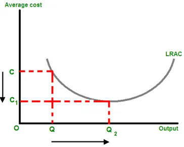
The increase in efficiency of production as the number of goods being produced increases is known as economies of scale. Typically, an agricultural company that achieves economies of scale lowers the average cost per unit through increased production since fixed costs are shared over an increased number of goods.
Economies of scale means that as a company grows and production units increase the company will have a better chance to decrease its costs.
Figure 1. The increase in output from Q to Q2 causes a decrease in the average cost of each unit from C to C1. Economies of scale are the cost advantages that a firm obtains due to expansion. This should not be confused with increasing returns to scale where simply increasing output within current capacity reduces the short run cost per unit.
Figure 1 shows a simple example and, in real life, there are countering forces of diseconomies of scale. Diseconomies of scale are the forces that cause larger firms to produce goods and services at increased per-unit costs. As these forces balance, an optimum production volume can be found referred to as constant returns to scale.
Economies of scale refers to the decreased per unit cost as output increases. More clearly, the initial investment of capital is spread over an increasing number of units of output, and therefore, the marginal cost of producing a good or service decreases as production increases (note that this is only in an industry that is experiencing economies of scale).
But Diseconomies Can Also Occur. As we mentioned before, diseconomies may also occur. They could stem from inefficient managerial or labour policies, over-hiring or deteriorating transportation networks (external DS). Furthermore, as a company's scope increases, it may
have to distribute its goods and services in progressively more dispersed areas. This can actually increase average costs resulting in diseconomies of scale.
Some efficiencies and inefficiencies are more location specific, while others are not affected by area. If a company has many plants throughout the country, they can all benefit from costly inputs such as advertising. However, efficiencies and inefficiencies can alternatively stem from a particular location, such as a good or bad climate for farming. When ES or DS are location specific, trade is used in order to gain access to the efficiencies.
The key to understanding economies of scale and diseconomies of scale is that the sources vary. A company needs to determine the net effect of its decisions affecting its efficiency, and not just focus on one particular source. Thus, while a decision to increase its scale of operations may result in decreasing the average cost of inputs (volume discounts), it could also give rise to diseconomies of scale if its subsequently widened distribution network is inefficient because not enough transport trucks were invested in as well. Thus, when making a strategic decision to expand, companies need to balance the effects of different sources of economies of scale and diseconomies of scale so that the average cost of all decisions made is lower, resulting in greater efficiency all around.
• Returns to scale
Refers to a technical property of production that examines changes in output subsequent to a proportional change in all inputs (where all inputs increase by a constant factor). If output increases by that same proportional change then there are constant returns to scale (CRTS). If output increases by less than that proportional change, there are decreasing returns to scale (DRS). If output increases by more than that proportion, there are increasing returns to scale (IRS)
Short example: where all inputs increase by a factor of 2, new values for output should be: Twice the previous output given = a constant return to scale (CRTS)
Less than twice the previous output given = a decreased return to scale (DRS) More than twice the previous output given = an increased return to scale (IRS)
• Allocative efficiency
Allocative efficiency is a situation in which the limited resources of a country are allocated in accordance with the wishes of consumers. An allocatively efficient economy produces an "optimal mix" of commodities.
A firm is allocatively efficient when its price is equal to its marginal costs in a perfect market. Allocative efficiency means efficient distribution of resources: an economic situation where no possible reorganization of production resources can make some consumers better off without making other consumers worse off.
If price information is available and a behaviour objective is appropriate, then it is possible to measure allocative efficiencies as well as technical efficiencies. Behaviour objectives could be cost minimisation or revenue or profit maximisation. Cost minimisation and revenue maximisation together imply profit maximisation.
• Factors which could influence the efficiency of a farm
These factors are not traditional inputs and are assumed not under the control of the manager. Some examples are:
• Ownership differences (public/private, corporate / noncorporate) • Coal-fired electric power station influenced by coal quality
• Electric power distribution networks influenced by population density and average customer size
• Schools influenced by socio-economic status of children and city/country location • Labour union power
• Government regulations.
DEA models
As we mentioned above the organizational units and farms are more generally called
DecisionMakingUnits (DMU)
.
DMUs can also be manufacturing units, departments of a big organization such as universities, schools, bank branches, hospitals, medical practitioners, power plants, police stations, tax offices, prisons, defence bases, or a set of firms. In the area of tourism DMUs can be hotels, motels, destinations, tourism websites, and so on.Efficiency of a decision making unit is defined as the ratio between a weighted sum of its outputs and a weighted sum of its inputs. We can find the DMU (or the DMUs) having the highest ratio. We call it DMUo. Then we can compare the performance of all other DMUs relative to the performance of DMUo. We can calculate the relative efficiency of the DMUs.
Suppose there are n DMUs, DMUj
,
j=1, 2, …, n. Suppose m input items and s output items are selected. Let the input data for DMUs be ij i mj nn
mX× =(x )=1,..., ; =1,...,
.
Let the input data forDMUs be
kj k s j n n
sY× =(y ) =1,...,; =1,...,
.
Given the data, we measure the efficiency of each DMUj
,
j=1,2,…,n. Hence we need noptimizations (one for each DMU to be evaluated).
Let the DMU, we are evaluating, be designated as DMUo
(o=1,2,…,n).
• CCR Model
We will define the CCR-Efficiency taking into account all input excesses and output shortfalls. The input oriented CCR model aims to minimise inputs while satisfying at least the given output levels. The output oriented CCR model attempts to maximise outputs without requiring more of any of the observed input variables.
Based on the matrix (X,Y), where X is an (m x n) matrix and Y is an (s x n) matrix, the Envelopment form of the CCR model is expressed as follows:
θ λ θ , min
subject to: θxo − Xλ ≥ 0
Yλ ≥ yo
λ≥0
where, for any DMUo o o mo T
mo x x x x ( 1 , 2 ,..., ) 1 = × , θ is a real variable, T n nλ×1=(λ1,...,λ ) is a non-negative vector.
For all DMUs together we have the following matrix notations:
1 × n θ
,
nλ
×n=(λ
jj)j=1,...,n;j=1,...,n, and n × 1 , minθ λθ subject to n m n n n m n mo X x × × × × × ≥ − 0 1 1 λ θ 1 1 × × ×nn ≥ so sY λ y1 1 0× × ≥n nλ
The optimal θ is denoted by θ*. It is greater than zero and not greater than 1, or 0<θ*≤1.
We define slack vectors by
1 1 1 1 1 × × × × × − = − n n m mo ms x θ X λ and ×1 × ×1 ×1 + = − so n n s s Y y s λ .
Definition: (CCR-Efficiency) If an optimal solution (θ*, λ*, s-*, s+*) of the CCR model satisfies θ*=1, s-*=0, s+*=0, then the DMUo is called CCR-efficient. Otherwise, the DMUo is called CCR-inefficient.
The condition θ*=1 is referred to as “radial efficiency”. The term “weak efficiency” is sometime used when attention is restricted to the condition θ*=1 (also called “Farrell efficiency”). The conditions θ*=1, s-*=0, and s+*=0, taken together describe what is also called “Pareto-Koopmans” or “strong” efficiency.
Definition: (Pareto-Koopmans Efficiency) A DMU is fully efficient if and only if it is not possible to improve any input or output without worsening some other input or output.
Definition: (Reference Set) For an inefficient DMUo, we define its reference set Eo by Eo = {j | λj* > 0}, j=1,…,n.
An optimal solution can be expressed as
* * 1 * 1 * 1 1 * 1 − ∈ × − × × × × = X +s =
∑
x +s x o E j j j m n n m mo λ λ θ* * 1 * * 1 1 + ∈ × + × × × − = − =Y s
∑
y s y o E j j j s n n s so λ λThe efficiency of (xo,yo) for DMUo can be improved by the formula:
1 1 * 1 1 * 1 1 ^ × × − × × × =mo −m ≤mo mxo x θ s x
1 1 * 1 1 ^ × × + × × ≥ + = so s so so y s y y
This formula for improvement is called the CCR projection. Theorem: The improved activity
(
,
)
^ ^
o
o
y
x
defined by the CCR projection is CCR efficient. Corollary to Theorem: The point with coordinates ( , )^ ^ o o y x
∑
∈ × − × × × = − = o E j j j m mo mxo x s x * 1 * 1 1 * 1 1 ^ λ θ∑
∈ × + × × = + = o E j j j s so so y s y y * 1 * 1 1 ^ λ• The output oriented CCR model
The output oriented CCR model attempts to maximize outputs while using no more than the observed amount of any input.
The slack (t‐, t+) of the output oriented model is defined by: µ X x t = o− − o y Y t+= µ−η η*
satisfies: η*≥1. The higher the value of η*, the less efficient the DMU is. η* expresses the output enlargement rate.
An input oriented CCR model is efficient for any DMU if and only if it is also efficient when the output oriented CCR model is used to evaluate its performance. The solution of the output oriented CCR model may be obtained from that of the input oriented CCR model.
The improvement using output oriented CCR model is expressed by:
∑
∈ − = − = o E j j j o o x t x x^ * µ*∑
∈ + = + = o E j j j o o y t y y * * * ^ η η• BCC Model
The BCC problem is solved using a two-phase procedure. In the first phase, we minimise θB
and, in the second phase, we maximise the sum of the input excesses and output shortfalls, keeping θB=θB*. Here θB* is the optimal value obtained in the first phase. An optimal BCC
solution is represented by (θB*, λ*, s-*, s+*), where s-* and s+* represent the maximal input
excesses and output shortfalls, respectively.
Definition: (BCC-efficiency) If an optimal BCC solution (θB*, λ*, s-*, s+*) satisfies θB*=1, s -*
=0, and s+*=0, then the DMUo is called BCC-efficient.
We have the following formula for improvement
x^o = θB*xo – s-*, y^o = yo + s+*
Theorem: The improved activity (x^o, y^o) is BCC-efficient.
• The Increasing ReturnstoScale Model (IRS) and the Decreasing ReturnstoScale
Model (DRS) or Relaxation of the convexity condition
The BCC envelopment model can be extended by relaxing the convexity condition eλ =1 to U
e
L≤ λ≤ , where L,(0≤ L≤1) and U,(1≤U) are lower and upper bounds for the sum of the λ . Notice that j L= U0, =∞ correspond to the CCR model and L= U =1 corresponds to the BCC model. Two typical extensions are discussed below.
The case L= U1, =∞ is called the Increasing Returns-to-Scale (IRS) or Non-Decreasing Returns-to-Scale (NDRS) model. The case L= U0, =1 is called the Decreasing Returns-to-Scale (DRS) or the Non-Increasing Returns-to-Returns-to-Scale (NIRS) model.
• The Increasing ReturnstoScale Model (IRS)
The constraint on λ is eλ ≥1. The interpretation of this constraint is that we cannot reduce the scale of DMU but it is possible to expand the scale to infinity. The output/input ratio for any point on the efficient frontier is not decreasing with respect to input. The term NDRS is derived from that fact. That is, a proportional increase in output is always at least as great as the related proportional increase in output is always at least as great as the related proportional increase in input. In mathematical terms
x x y
y ≥ ∆ ∆
, where ∆ ,y ∆x are the increases to be made from a frontier point with coordinate (x,y). This model focuses on the scale efficiencies of
relatively small DMUs.
• The Decreasing ReturnstoScale (DRS) Model
The constraints on λ are 0≤eλ≤1. The interpretation of these constraints is that scaling up of DMUs is interdicted, scaling down is permitted. The output/input ratio of efficient frontier points is decreasing with respect to the input scale. That is
x x y
y = ∆ ∆
for the first segment on
the frontier and strict inequality
x x y
y < ∆ ∆
holding thereafter. This model puts the emphasis on larger DMUs where returns to scale is decreasing.
It is logically true that for every DMU we have the relations * * * *
, DRS BCC IRS
CCR θ θ θ
• Model Sources of Inefficiency
It is interesting to investigate the sources of inefficiency that a DMU might have. Are they caused by the inefficient operation of the DMU itself or by the disadvantageous conditions under which the DMU is operating?
For this purpose, comparisons of the (input-oriented) CCR and BCC scores deserve consideration. The CCR model assumes the constant returns-to-scale production possibility set. It is postulated that the radial expansion and reduction of all observed DMUs and their nonnegative combinations are possible and hence the CCR score is called global technical efficiency. The BCC model assumes that convex combinations of the observed DMUs form the production possibility set and the BCC score is called local pure technical efficiency. If a DMU is fully efficient in both the CCR and BCC scores, it is operating in the most productive scale size.
If a DMU has full BCC efficiency but a low CCR score, then it is operating locally efficiently but not globally efficiently due to the scale size of DMU. Thus, it is reasonable to characterize the scale efficiency of a DMU by the ration of CCR and BCC scores. We define scale efficiency as follows:
Definition: Let the CCR and BCC scores of a DMU be θCCR* and
*
BCC
θ , respectively. The scale efficiency SE is defined by * * BCC CCR SE θ θ = .
SE is not greater than 1. The BCC score expresses the (local) pure technical efficiency (PTE) under variable returns-to-scale circumstances. The CCR score is called the (global) technical efficiency (TE), since it takes no account of scale effect as distinguished from PTE. For a BCC-efficient DMU with constant returns-to-scale characteristics (i.e., in the most productive scale size) the scale efficiency SE is 1.
• SBM model
We introduce a new measure ρ called SBM (Slacks-Based Measure). It is invariant to the units of measure used for the different inputs and outputs. This new measure is a scalar that yields the same efficiency value when distances are measured in either kilometres or miles.
More generally, this measure is the same when xio and xij are replaced by kixio= x^io and kixij =
x^ij and yro and yrj are replaced by cryro= y^ro and cryrj = y^rj , where ki and cr are positive
constants, i=1,…,m, r=1,…,s. This property is known as “units invariant”. The SBM measure is monotone decreasing in each input and output slack. This property is known as “monotone”.
Slacks-Based Measure ρ can be interpreted as the ratio of mean input and output mix inefficiencies.
Theorem: If DMU A dominates DMU B so that xA≤xB and yA≥ yB, then ∗ ≥ ∗
B
A ρ
ρ .
Definition: (SBM-efficient) A DMU (xo ,yo) is SBM-efficient if and only if ρ* =1.
This condition is equivalent to s-* =0 and s+* =0, i.e. no input excess and no output shortfall in an optimal solution.
For an SBM-inefficient DMU (xo ,yo), we have the expression:
xo = Xλ* + s-*,
yo= Yλ* - s+*.
The DMU (xo ,yo) can be improved and becomes efficient by deleting the input excesses and
augmenting the output shortfalls. This is accomplished by SBM-projection expressed by the following formulae, called SBM-projection:
x^o = xo - s-*,
y ^o= yo + s+*,
which are the same as for the Additive model. We will define the reference set for (xo,yo) as:
Definition: (Reference set) The set of indices Ro corresponding to positive λj*s is called the
reference set for (xo,yo).
Using the reference set Ro we can express ( , ) ∧ ∧ o o y x by:
∑
∈ ∗ ∧ = o R j j j o x x λ∑
∈ ∗ ∧ = o R j j j o y y λThis means that the point on the efficient frontier ( , ) ∧ ∧ o o y x is expressed as a positive combination of the members of the reference set Ro. The members of the reference set Ro are
also efficient.
Theorem: The optimal SMB ρ*
is not greater than the optimal CCR θ*.
This theorem reflects the fact that SBM accounts for all inefficiencies whereas θ* accounts only for “purely technical“ inefficiencies.
The relation between CCR-efficiency and SMB-efficiency is given in the following theorem: Theorem: A DMU (xo ,yo) is CCR-efficient if and only if it is SMB-efficient.
• Outlier detection in PAR
The main drawback of deterministic frontier models is that they are very sensitive to outliers and extreme values, and that noisy data are not allowed. We perform outlier analysis using the method described in (Wilson, 1993). This paper describes an influence-function approach for detecting outliers in the context of frontier models.
The graphic analysis based on outlier statistic developed in (Wilson,1993) and implemented in FEAR is used to identify observations in DEA models that are possible outliers. A line in the log-ratio plot connects the second smallest value of the ratios for each observation deleted to illustrate the separation between the smallest rations for each observation. The plot is approximately linear under the homogeneity model. Under the heterogeneity model, the log-ratio plot shows convexity.
• Some notes on CCA and some related methods
Canonical Correlation Analysis (CCA) is a multidimensional exploratory statistical method. A canonical correlation is the correlation of two latent (canonical) variables, one representing a set of independent variables, the other a set of dependent variables. Each set may be considered a latent variable based on measured original variables in its set. The canonical correlation is optimized such that the linear correlation between the two latent variables (called canonical variates) is maximized. There may be more canonical variates relating the two sets of variables. The purpose of canonical correlation is to explain the relation of the two sets of variables, not to model the individual variables. For each canonical variate we can also
assess how strongly it is related to measured variables in its own set, or the set for the other canonical variate.
Both methods Principal Components Analysis (PCA) and CCA have the same mathematical background. The main purpose of CCA is the exploration of sample correlations between two sets of quantitative variables, whereas PCA deals with one data set in order to reduce dimensionality through linear combination of initial variables.
Another well known method can deal with the same kind of data: Partial Least Squares (PLS) regression. However, the object of PLS regression is to explain one or several response variables (outputs) in one set, by way of variables in the other one (the input). On the other hand, the object of CCA is to explore correlations between two sets of variables whose roles in the analysis are strictly symmetric. As a consequence, mathematical principles of both PLS and CCA methods are fairly different.
• Variable aggregation in PAR
The question of obtaining an appropriate aggregate input from appropriate individual inputs is an important one. A natural way to define an aggregate input is to assume a linear structure of aggregation of the input variables. One of the most important issues here is the choice of weights in the aggregation.
A natural extension of the aggregation of inputs or outputs techniques is the use of weight restrictions. The use of weight restrictions is a much more subtle technique. For example, instead of eliminating an unimportant input or output, which is, the same as assigning a zero weight to it, we may restrict its weight to be low in relation to the more important inputs and outputs. This way the unimportant parameter will still count in the overall model but only up to the specified limit of ‘importance’.
Weights choice may be done by the researcher according his opinion about the contribution of each variable. In our approach we use Canonical Correlations Analysis (CCA) to aggregate automatically both input and output data sets.
Obviously the input and output sets of variables in a production process are related. We are concerned with determining a relationship between the two sets of variables. The aim is the linear combinations that maximize the canonical correlation to be fond. Such a linear combination is called “canonical variate”.
In this paper, we propose CCA to aggregate both input and output variables to get final input and output, respectively.
The aggregation in PAR approach is not fixed and because of it we are giving the answer of the following two important questions that arise frequently.
• Variable selection in PAR
Variable selection in DEA is problematic. The estimated efficiency for any DMU depends on the inputs and outputs included in the model. It also depends on the number of outputs plus inputs. It is clearly important to select parsimonious specifications and to avoid as far as possible models that assign full high efficiency ratings to DMUs that operate in unusual ways. In practice, when we apply DEA the number of DMUs should be greater that the total amount of variables in both sets. Usually in real world applications the number of DMUs is restricted. Because of it one of the most important steps in the modelling using DEA is the choice of input and output variables.
Variable selection is crucial to the process as the omission of some of the inputs can have a large effect on the measure of efficiency. It is now recognized that improper variable selection often results in biased DEA evaluation results.
The attention to variable selection is particularly crucial since the greater the number of input and output variable, the less discerning are the DEA results (Jenkins and Anderson, 2003). However, there is no consensus on how best to limit the number of variables.
Several methods have been proposed that involve the analysis of correlation among the variables, with the goal of choosing a set of variables that are not highly correlated with one another. Unfortunately, studies have shown that these approaches yield results which are often inconsistent in the sense that removing variables that are highly correlated with others can still have a large effect on the DEA results (see Nunamaker, 1985). Other approaches look at the change in the efficiencies themselves as variables are added and removed from the DEA models, often with a focus on determining when the changes in the efficiencies can be considered statistically significant. As part of these approaches, procedures for the selection of variables to be included in the model have been developed by sequentially applying statistical techniques.
Another commonly used approach for reducing the list of variables for inclusion in the DEA model is to apply regression and correlation analysis (Lewin et al., 1982. This approach purports those variables which are highly correlated with existing model variables are merely redundant and should be omitted from further analysis. Therefore, a parsimonious model typically shows generally low correlations among the input and output variables, respectively (Chilingerian, 1995 and Salinas-Jimenez and Smith, 1996).
The authors Norman and Stoker (1991) noted that the observation of high statistical correlation alone was not sufficient. A logical causal relationship to explain why the variable influenced performance was necessary. Another application of variable selection based on correlating the efficiency scores can be found in Sigala et al. (2004).
In this paper, we propose CCA to be used in order the most appropriate variables to be selected. In PAR approach we apply CCA to select both input and output variables and to get final input and output sets, respectively.
Azorean Farms’ Efficiency Measurement
The Azores islands belong to the Portuguese territory with a population of about 250000 inhabitants. The main economic activity is dairy and meat farming. Dairy policy depends on Common Agricultural Policy of the European Union and is limited by quotas. In this context, decision makers need knowledge for deciding the best policies in promoting quality and best practices. One of the goals of our work is to provide Azorean Government with a reliable tool for measurement of productive efficiency of the farms.
The names of all input variables used in analysis are the following: EquipmentRepair, Oil, Lubricant, EquipmentAmortization, AnimalConcentrate, VeterinaryAndMedicine, OtherAnimalCosts, PlantasSeeds, Fertilizers, Herbicides, LandRent, Insurance, MilkSubsidy, MaizeSubsidy, SubsidyPOSEIMA, AreaDimension, and DairyCows. The names of output variables are Milk and Cattle.
We start the data analysis with outlier detection. One outlier obtained in Terceira data was result of a recording error and was corrected. We used again the statistical methodology presented in (Wilson, 1993) and implemented in FEAR package to look for new atypical observations. Using the graphical analysis presented in Figure another observation could also
be identified as an outlier. However data from Terceira Island are viewed as having come from a probability distribution and it is quite possible to observe one point with low probability. One would not expect to observe many such
points, given their low probability. The fact that a particular observation has low probability of occurrence is not sufficient to warrant the conclusion that this observation is an error. More errors in the available data are not identified. Figure 2. Plot produced by the outlier detection procedure.
Canonical correlation analysis aims at highlighting correlations between input and output data sets. Two preliminary steps calculate the sample correlation coefficients and visualise the correlation matrixes. All sample correlation coefficients are presented in Table 1.
This table highlights a significant correlation between Milk and AnimalConcentrate and nearly null correlation between Milk and Lubricant, Milk and EquipmentAmortization, and Milk and Insurance.
In practice, the number of DMUs should be greater that the total amount of variables in both input and output sets. Any resource used by an Azorean dairy farm is treated as an input variable and because of it the list of variables that provide an accurate description of the milk and meat production process is large.
Table 1 Sample correlation coefficients. Milk Cattle EquipmentRepair 0.399089550 0.449336923 Oil 0.349190515 ‐0.023206764 Lubricant 0.009272362 ‐0.171455723 EquipmentAmortization 0.051043354 ‐0.077088336 AnimalConcentrate 0.914685924 0.537983929 VeterinaryAndMedicine 0.707943660 0.370392398 OtherAnimalCosts 0.724266952 0.407358115 PlantasSeeds 0.719946680 0.304399253 Fertilizers 0.781448807 0.452145566 Herbicides 0.497643020 0.347245965 LandRent 0.722516988 0.343699321 Insurance ‐0.072519332 0.002379461 MilkSubsidy 0.746508776 0.431464776 MaizeSubsidy 0.751413121 0.526768325 SubsidyPOSEIMA 0.724407535 0.083726114 AreaDimension 0.536678292 0.279164537 DairyCows 0.776032879 0.348513730
This example is focused on measuring efficiency when the number of DMUs is few and the number of explanatory variables needed to compute the measure of efficiency is too large. We approach this problem from a statistical standpoint through both variable selection and variable aggregation approaches.
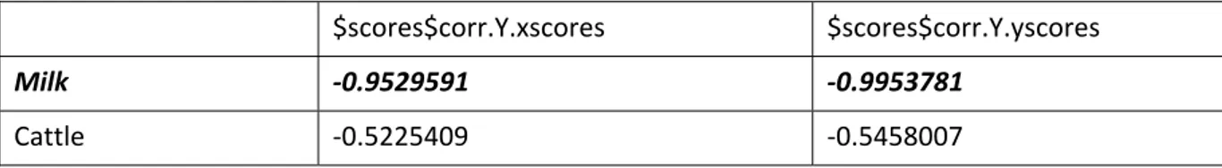
The results from CCA are printed in the Appendix and in the following tables. Table 2 Correlations of the original outputs with both aggregated input and output.
$scores$corr.Y.xscores $scores$corr.Y.yscores
Milk ‐0.9529591 ‐0.9953781
$scores$corr.X.xscores $scores$corr.X.yscores EquipmentRepair ‐0.44487248 ‐0.42591381 Oil ‐0.34213524 ‐0.32755482 Lubricant 0.01024649 0.00980983 EquipmentAmortization ‐0.04167289 ‐0.03989696 AnimalConcentrate ‐0.96395974 ‐0.92287966 VeterinaryAndMedicine ‐0.74087590 ‐0.70930276 OtherAnimalCosts ‐0.76117503 ‐0.72873682 PlantasSeeds ‐0.74525915 ‐0.71349921 Fertilizers ‐0.82269954 ‐0.78763940 Herbicides ‐0.53062365 ‐0.50801061 LandRent ‐0.75224389 ‐0.72018629 Insurance 0.07133021 0.06829041 MilkSubsidy ‐0.78586254 ‐0.75237225 MaizeSubsidy ‐0.80148885 ‐0.76733263 SubsidyPOSEIMA ‐0.72469294 ‐0.69380945 AreaDimension ‐0.56145996 ‐0.53753280 DairyCows ‐0.80562574 ‐0.77129323
From Table 2 we can conclude that both canonical variates are predominantly associated with the following original inputs: Animal Concentrate and Fertilizers, and with the original output variable Milk. In this way we select the following two input variables Animal Concentrate and Fertilizers, and one output variable Milk.
On Figure 3 the input and output variables are plotted on the first two canonical variates. Variables with a strong relation are projected in the same direction from the origin. The greater the distance from the origin, the stronger the relation is. The following variables: AnimalConcentrate, VeterinaryAndMedicine, OtherAnimalCosts, MilkSubsidy, MaizeSubsidy, Herbicides, Fertilizers, PlantasSeeds, LandRent, AreaDimension, DairyCows and Milk are a set of variables with a stronger relation than the rest. In this set AnimalConcentrate, DairyCows, VeterinaryAndMedicine, OtherAnimalCosts and MilkSubsidy are the variables with most strong relation. MaizeSubsidy and Herbicides are also variables with a strong relation.
Figure 3. The input and output variables plotted on the first two canonical variates.
Both, the original inputs and outputs are aggregated into overall measures called aggregate input variate and aggregate output variate.
Then we use aggregated input and output in DEA formulation.
We build the DEA analysis on aggregated measures. On Figure 4 all DMUs and the efficient frontier are visualised.
Figure 4. Several examples with and without aggregation using BCC Model (first two) and CCR model
Conclusions
PAR (Productivity Analysis with R) is implemented in R statistical software version 2.8.1 using the DEA, FEAR and CCA packages and routines developed by us (see R Development Core Team, 2007). PAR is very flexible, extensible software based on CCA and DEA models, implemented as CCA and FEAR packages in R. The cost of this flexibility is that the user must type commands at a command-line prompt.
In PAR methodology CCA provides an aggregation of both input and output units and then DEA provides efficient units. The aggregation can cause significant additional bias in an DMU’s technical efficiency scores. The effects of the input aggregation on efficiency indicators have been investigated. This study used data from Terceira Island. Azorean government can apply our approach to other islands and to find “the best practice” of Azorean agricultural system.
In spite of the good results achieved is important to recognize the major limitations and possible problems in conducting a DEA.
• Measurement error and other noise may influence the shape and position of the frontier.
• The exclusion of an important input or output can result in biased results. Because of it a variable aggregation method is proposed by PAR.
• The efficiency scores obtained are only relative to the best firms in the sample. The inclusion of extra firms (e.g., from overseas) may reduce efficiency scores.
• Be careful when comparing the mean efficiency scores from two studies. They say nothing about the efficiency of one sample relative to the other.
• The addition of an extra firm in a DEA analysis cannot result in an increase in the TE scores of the existing firms.
• The addition of an extra input or output in a DEA model cannot result in a reduction in the TE scores.
• With few observations and many inputs and/or outputs many of the firms will appear on the DEA frontier. If an investigator wishes to make an industry look good, he could reduce the sample size and increase the number of inputs and outputs in order to increase the TE scores. Because of it a variable selection method is proposed by PAR. • Treating inputs and outputs as homogeneous commodities when they are
heterogeneous may bias results.
In future work we are going to use PAR with both real and simulated data in order to find out a compromise between environment, agriculture and tourism, and to investigate the potential impact of agricultural tourism on the farms efficiency.
Acknowledgments
This work has been partially supported by Regional Division for Science and Technology of Azores Government through the project M.2.1.2/l/009/2008, "Productivity Analysis of Azorean Cattle-Breeding Farms with R Statistical Software".
Bibliografia
Bauernfeind, Ulrike; Mitsche, Nicole. The Application of the Data Envelopment Analysis for Tourism Website Evaluation. Information Technology & Tourism, Volume 10, Number 3, 2008 , pp. 245‐257(13) Chilingerian J.A. (1995) Evaluating physician efficiency in hospitals: A multivariate analysis of best practices. European Journal of Operational Research 80 pp. 548–574 Coelli T., Rao D., Battese (1998) “An Introduction to Efficiency and Productivity Analysis”, Kluwer Academic Pub. Coelli T.J. (1996) “Assesing the Performance of Australian Universities using Data Envelopment Analysis”, University of New England.Cooper, W. W., Seiford, L. M. and Tone, K. (2007). “Data envelopment analysis: a comprehensive text with models, applications, references and DEA‐solver software”. Second edition. Springer. New York. Diaz‐Martinez, Zuleyka and Jose Fernandez‐Menendez (2008). “DEA: Data Envelopment Analysis. R package” version 0.1‐2. Diaz‐Martinez, Zuleyka and Jose Fernandez‐Menendez (2009) “The DEA Package”. Version 0.1‐2, March http://cran.r‐project.org/web/packages/DEA/DEA.pdf Garzon, Izabelle (2005) “Multifunctionality of Agriculture in the European Union: Is there substance behind the discourse’s smoke?” Institute of Governmental Studies (University of California, Berkeley). Paper WP2005‐36 Gimenez‐Garcia V.M., José Luis Martínez‐Parra, Frank P. B. (2007) Improving resource utilization in multi‐unit networked organizations: The case of a Spanish restaurant chain. Tourism management, vol. 28, pp 262 ‐270 Jenkins, L and M Anderson (2003). A multivariate statistical approach to reducing the number of variables in data envelopment analysis. European Journal of Operational Research, 147, 51‐61. Levine, Mark S. (1977) “Canonical analysis and factor comparison”. Thousand Oaks, CA: Sage Publications, Quantitative Applications in the Social Sciences Series, No. 6. Lewin. A.Y. Lewin, R.C. Morey and T.J. Cook, (1982) Evaluating the administrative efficiency of courts, OMEGA 10 (1982) (4), pp. 401–411. Mendes A., V. Noncheva, E. Silva (2009). Decision Support for Enhanced Productivity with R Software: An Azorean Farms Case Study, Thirty Eighth Annual Meeting of WDSI, Hawaii, April 7‐11, 2009. Norman M. and B. Stoker (1991) “Data Envelopment Analysis: The assessment of performance” John Wiley and Sons, Chichester, England. Nunamaker, T.R. (1985). Using data envelopment analysis to measure the efficiency of non‐profit organizations: A critical evaluation, Managerial and Decision Economics 6 (1985) (1), pp. 50–58. Organisation for Economic Co‐Operation and Development (OCDE) (2001) “Environmental Indicators for Agriculture Methods and Results”. Executive summary. Rodriguez, M.; E. Gómez, J. Lorente (2004) “Rural Multifunctionallity in Europe. The concepts and policies” 90th AEEA Seminar. Salinas‐Jimenez, J. and P. Smith (1996) Data envelopment analysis applied to quality in primary health care. Annals of Operations Research 67, pp. 141–161 Shephard, R.W. (1953) “Cost and Production Functions” Princeton University Press, Princeton. Shephard, R.W. (1970) “Theory of Cost and Production Functions” Princeton University Press, Princeton. Sigala, M.; D. Airey, P. Jones and A. Lockwood (2004). ICT paradox lost? A stepwise DEA methodology to evaluate technology investments in tourism settings, Journal of Travel Research 43, pp. 180–192. Simar, L., and Wilson, P.W. (2000). A general methodology for bootstrapping in non‐parametric frontier models, Journal of Applied Statistics, 27, 779‐802. SREA (2007) “Estudo sobre os Turistas que visitam os Açores. 2005 – 2006”. Região Autónoma dos Açores / ed. Serviço Regional de Estatística dos Açores. SREA (2007a) “Anuário Estatístico dos Açores, 2007” Região Autónoma dos Açores / ed. Serviço Regional de Estatística dos Açores. Wilson, P. W (1993) Detecting outliers in deterministic nonparametric frontier models with multiple outputs. Journal of Business and Economic Statistics, 11, pp. 319‐323. Wilson, P. W. (2005) “FEAR 1.0 : A Software Package for Frontier Efficiency Analysis with R”, http://business.clemson.edu/Economic/faculty/wilson/courses/bcn/papers/fear.pdf Wilson, P. W. (2007) “FEAR 1.0 : A Software Package for Frontier Efficiency Analysis with R” Socio‐Economic Planning Sciences. Forthcoming.
Appendix
$names $names$Xnames [1] "t.EquipmentRepair" "t.Oil" "t.Lubricant" "t.EquipmentAmortization" "t.AnimalConcentrate" [6] "t.VeterinaryAndMedicine" "t.OtherAnimalCosts""t.PlantasSeeds" "t.Fertilizers" "t.Herbicides" [11] "t.LandRent" "t.Insurance" "t.MilkSubsidy" "t.MaizeSubsidy" "t.SubsidyPOSEIMA" [16] "t.AreaDimension" "t.DairyCows" $names$Ynames [1] "t.Milk" "t.Cattle" $names$ind.names [1] "1" "2" "3" "4" "5" "6" "7" "8" "9" "10" "11" "12" "13" "14" "15" "16" "17" "18" "19" "20" "21" "22" "23" "24" "25" "26" "27" "28" "29" "30" $xcoef [,1] [,2] t.EquipmentRepair 2.839421e-05 6.236793e-04 t.Oil 1.549179e-05 -1.074609e-04 t.Lubricant 1.199566e-03 1.571479e-04 t.EquipmentAmortization -3.131292e-06 -8.008881e-05 t.AnimalConcentrate -8.497169e-05 1.945530e-04 t.VeterinaryAndMedicine 1.473172e-05 -9.457584e-04 t.OtherAnimalCosts -5.441544e-06 -4.647821e-04 t.PlantasSeeds -1.021208e-04 3.622781e-05 t.Fertilizers -1.305625e-06 1.098682e-04 t.Herbicides 6.589684e-04 4.378876e-04 t.LandRent 2.583145e-05 -2.461932e-04 t.Insurance 1.655867e-04 -7.351506e-05 t.MilkSubsidy 2.115323e-05 -1.552171e-04 t.MaizeSubsidy -3.555158e-04 7.228373e-04 t.SubsidyPOSEIMA -6.560970e-05 -4.479321e-04 t.AreaDimension 3.092947e-04 2.763918e-04 t.DairyCows -2.520118e-02 -1.683335e-02 $ycoef
[,1] [,2] t.Milk -3.419875e-05 -2.227637e-05 t.Cattle -3.778954e-05 3.916862e-04 $scores $scores$xscores [,1] [,2] [1,] 0.106668343 0.310173549 [2,] 0.462835833 -1.766860604 [3,] 0.794871641 0.533469101 [4,] -0.120125963 -0.919913579
[6,] -0.026970821 -0.282813393 [7,] -0.864746787 -0.390075060 [8,] -0.792695420 -0.290506622 [9,] 0.585106678 0.005449548 [10,] 0.017996307 -0.928991450 [11,] -1.107011122 2.890541608 [12,] 0.496400464 -0.144078944 [13,] 0.703610166 -1.155951762 [14,] 0.999781479 1.171387332 [15,] 0.846128147 -0.426472457 [16,] 0.250199227 -0.136025611 [17,] -0.064930903 -0.236511190 [18,] 0.554410123 -0.139607304 [19,] -0.152425124 0.569498433 [20,] -4.525830693 -0.464054783 [21,] -0.393858209 -0.174933953 [22,] 0.084126849 0.895744988 [23,] 0.439480570 0.546899526 [24,] 0.009491117 0.092598957 [25,] 0.219187073 -1.632006421 [26,] 0.042780367 -0.158701611 [27,] 0.843920501 -0.575147439 [28,] 0.394922946 2.652382611 [29,] -0.075265721 -0.020825726 [30,] -0.378553014 -0.337027569 $scores$yscores [,1] [,2] [1,] 0.01149440 0.61153890 [2,] 0.23104478 -0.91273800 [3,] 1.18001017 0.78486851 [4,] 0.24058177 -0.98562309 [5,] 0.64783956 -0.15625512 [6,] -0.16402876 -0.23132094 [7,] -0.65490565 -0.64808720 [8,] -0.30673390 0.39620853 [9,] 0.43536519 -0.36912461 [10,] 0.39464496 -0.55585425 [11,] -1.23000488 2.49215933 [12,] 0.02372779 -0.42540930 [13,] 0.32175703 -0.44567441 [14,] 1.22651631 1.13299121 [15,] 0.68979748 -0.22259243 [16,] 0.20603813 -0.97273848 [17,] 0.43996483 0.07156259 [18,] 0.48826837 -1.07444066 [19,] 0.33999751 0.39162471 [20,] -4.44746778 -0.58920753 [21,] -0.08845697 -0.72536849 [22,] -0.12988248 -0.05712870 [23,] 0.18264542 -0.46468501 [24,] -0.05068773 0.46853297 [25,] 0.03653218 -1.19347110 [26,] -0.05962358 -0.22367726 [27,] 1.03199677 -0.66199319
[28,] 0.25887008 2.75668410 [29,] -0.28948440 2.01408524 [30,] -0.96581662 -0.20486634 $scores$corr.X.xscores [,1] [,2] t.EquipmentRepair -0.44487248 0.32218146 t.Oil -0.34213524 -0.30006653 t.Lubricant 0.01024649 -0.24675670 t.EquipmentAmortization -0.04167289 -0.14687034 t.AnimalConcentrate -0.96395974 0.05091896 t.VeterinaryAndMedicine -0.74087590 -0.02487685 t.OtherAnimalCosts -0.76117503 0.01428088 t.PlantasSeeds -0.74525915 -0.12631740 t.Fertilizers -0.82269954 0.03305618 t.Herbicides -0.53062365 0.10395092 t.LandRent -0.75224389 -0.07335618 t.Insurance 0.07133021 0.05890674 t.MilkSubsidy -0.78586254 0.03092890 t.MaizeSubsidy -0.80148885 0.16037941 t.SubsidyPOSEIMA -0.72469294 -0.43817945 t.AreaDimension -0.56145996 -0.02112679 t.DairyCows -0.80562574 -0.10764300 $scores$corr.Y.xscores [,1] [,2] t.Milk -0.9529591 -0.07714827 t.Cattle -0.5225409 0.67313882 $scores$corr.X.yscores [,1] [,2] t.EquipmentRepair -0.42591381 0.25882440 t.Oil -0.32755482 -0.24105837 t.Lubricant 0.00980983 -0.19823193 t.EquipmentAmortization -0.03989696 -0.11798825 t.AnimalConcentrate -0.92287966 0.04090573 t.VeterinaryAndMedicine -0.70930276 -0.01998481 t.OtherAnimalCosts -0.72873682 0.01147254 t.PlantasSeeds -0.71349921 -0.10147705 t.Fertilizers -0.78763940 0.02655567 t.Herbicides -0.50801061 0.08350894 t.LandRent -0.72018629 -0.05893067 t.Insurance 0.06829041 0.04732272 t.MilkSubsidy -0.75237225 0.02484672 t.MaizeSubsidy -0.76733263 0.12884076 t.SubsidyPOSEIMA -0.69380945 -0.35201136 t.AreaDimension -0.53753280 -0.01697220 t.DairyCows -0.77129323 -0.08647498 $scores$corr.Y.yscores [,1] [,2] t.Milk -0.9953781 -0.09603322 t.Cattle -0.5458007 0.83791500