An efficient algorithm eradicating semantic
gap with help of image quality assessment
ASHISH OBEROI
Department of Computer Engineering, M.M. Engineering College,
M.M. University,
Mullana-133 207, Ambala, Haryana, India
EKTA WALIA
Prof. & Head, Department of Information Technology M.M. Engineering College,
M.M. University,
Mullana-133 207, Ambala, Haryana, India Abstract:
Early retrieval systems are lacking in recognizing the existence of semantic gap. If we have better image quality measure, we are able to reduce the semantic gap significantly. To evaluate the performance of image, image quality measures are used. The subjective evaluation is the only way to assess image quality. This can be done by human observers. In this the mean value of their scores is used as the quality measure. This is called mean opinion score (MOS). In these measures there are various objective (quantitative) measures. There are many quantitative measures and many other quality measures have been proposed. These measures have some advantages over MSE (mean squared error), but their ability to predict image quality is still limited. A different approach is presented here. Quality measure proposed here uses simple model of HVS, which has one user-defined parameter, whose value depends on the reference image. This quality measure is based on the average value of locally computed correlation coefficients. This takes into account structural similarity between original and distorted images, which cannot be measured by MSE or any kind of weighted MSE. The proposed measure also differentiates between random and signal dependant distortion, because these two have different effect on human observer. In this we have to give original image and our algorithm will produce a better quality of image in case of distortion or in the case of noise. Thus, with the help of this algorithm semantic gap can be reduced significantly.
Keywords: Mean opinion score (MOS); Mean squared error (MSE); Contrast sensitivity function (CSF); Peak signal to noise ratio (PSNR); Signal to noise ratio (SNR).
1. Introduction
sensitivity function) and texture masking. One such algorithm is described in [9]. In this approach input intensities are first modified by a nonlinear function modeling brightness perception and then filtered by a 2-D filter modeling frequency response of HVS. Also, this algorithm does not produce one number that indicates image quality. Image quality measures are sometimes developed as a part of image processing algorithms. An example of this can be found in [10], where properties of HVS are used to design an algorithm for image coding. Another approach is presented in [9]. It is assumed here that input image is degraded by two sources of degradation: linear distortion (for example as a result of filtering) and additive noise. An overview of image quality measures is presented in [9]. Performance of several proposed quality measures is tested in [13]. Distorted images are created using four different image coding algorithms, which produce different types of degradation. Then tested quality measures are computed for each distorted image and these values are compared with subjective assessment. The tested measures included MSE and the measure proposed in [10]. The quality measure from [10] showed best agreement with subjective evaluation compared with other tested measures. However, none of the tested measures was able to predict subjective image quality consistently.
In [12] and [13] previously proposed quality measures are discussed and it is noted that these measures frequently use some problematic assumptions. Also it is pointed out that MSE or some modifications of MSE (such as the one described in [10]) completely fail to measure structural similarity between two images, which is very important for a human observer. In other words MSE computes only error between the corresponding pixels but does not take into account correlation between that pixel and surrounding pixels in any of the two input images. It is possible to introduce a very large MSE by shifting the mean value of image intensities or by contrast stretching and preserve structural similarity between the two images. On the other hand if the same amount of MSE is introduced as a result of low-pass filtering or image coding, the resulting image can be severely distorted. Algorithms described in [1], [10] and [3] do not measure structural similarity at all. Based on this discussion a new image quality measure is proposed in [12] and [13]. This measure is computed locally and it is defined as a product of three components. Most important of these components is correlation coefficient, which measures the degree of linear relationship between the corresponding blocks of pixels. Quality measure for the whole image is the average value of locally computed quality measures. This approach does not use HVS model at all.
2. System model
The approach presented here will use some ideas from [12] and [13], but it will not use image quality measure as it is defined there (only correlation coefficient will be used). In the first step original image and distorted image are processed by simple model of HVS which consists of a nonlinear function modeling brightness perception and a degradation filter modeling frequency response of HVS (contrast sensitivity function). The degradation used in this HVS model is not fixed. It contains one user-defined parameter which can be changed depending on the context of the reference image. After this, the correlation coefficient can be computed on a block-by-block basis for the processed input images. Finally, quality measure can be computed as the average correlation coefficient between the original image and distorted image, adjusted by average correlation coefficient between the original image and error image. In this we take the original image then it will give the value according to this efficient Algorithm.
2.1 Simple HVS model
The simple model of HVS shown in Figure 1, which models brightness perception and frequency response of HVS. The output signal in this case depends on the viewing distance, the width and the height and the number of pixels of the input image. This is reasonable because image perception by HVS also depends on these parameters.
Nonlinear Function
f(m,n) p(m,n) x(m,n) y(m,n)
2D Filter
Figure: 1 (Architecture of HVS Model)
Nonlinear Function
f(m,n) p(m,n) x(m,n) y(m,n)
Degradation
This architecture works as same to the previous model. In this the function is passed to nonlinear function. This function gives the value as to the function. This is passed to degradation where the quality of image is passed. That gives the reference image after distortion. The objective of this research is to develop an image quality measure, which will produce results that are in agreement with subjective assessment and ultimately reduces the semantic gap [11].
2.1.1 Algorithm
Step1: Given the original image f(m, n), distorted image p(m, n), width, height and number of pixels of the input images and viewing distance, compute images x(m, n) and y(m, n) using the described model of HVS.
Step 2: Compute the error between images x (m, n) and y (m, n) as the average value of locally computed correlation coefficients between images x (m, n) and y(m, n).
Step 3: Compute the average correlation coefficient as the average value of the locally computed correlation coefficients between images x (m, n) and y (m, n).
Step 4: Find the image quality measure
2.2 Contrast sensitivity function (CSF)
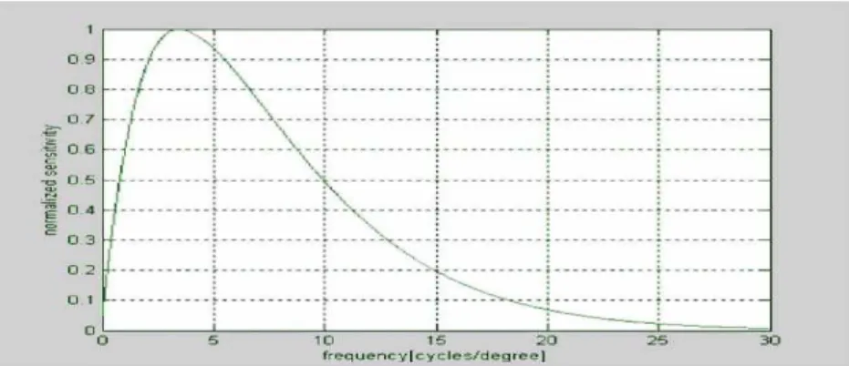
It describes the frequency response of HVS is not equally sensitive to all spatial frequencies. Various functions have been suggested to model this effect. Most of them have a band-pass character but they have maximum at different frequencies. For example CSF shown in [9] has maximum at 3 cycles/degree, while CSF used in [12] has maximum at 8 cycles/degree. It is also noted in [8] that various CSF suggested by different authors have maximum at frequencies ranging from 3 to 10 cycles/degree. Since there is no reliable way to tell which one of these functions represents the best model of HVS, none of them will be used here. Instead, CSF used for f = 3. 5 cycles/degree. In the last formula, f denotes frequency in cycles/degree and the parameter which controls the rate at which CSF decreases after it reaches its maximum at 3.5 cycles/degree is set to 0.75. This function is shown in Figure 3:
Figure 4: Contrast sensitivity function in case of complex Image
Although the previous experiment with the sequence of “Lena” images shows that HVS is frequency selective, we must be cautious with this interpretation. This example shows that noise at high frequencies is less visible than noise at low frequencies. This requires some user intervention but it yields better results.
3. Results
3.1. “Lena” image with various types of distortion
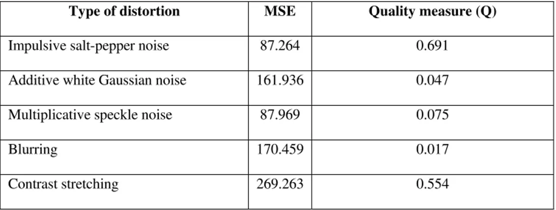
Performance of the algorithm will be illustrated by several examples. In all examples, the following parameter values will be used: image height and width of 15 cm, viewing distance of 60 cm and image size of 512x512 pixels. Parameter which controls the rate at which CSF decreases after it reaches its maximum at 3.5 cycles/degree will depend on the original image. First example will be the sequence of “Lena” images with various types of distortion shown in table 1. For this image, we set a=0.75. All images in the sequence have the same MSE value of 225 (except for JPEG coded image, which has MSE of 215), but their visual quality is very different. The results are shown in table 1.
Type of distortion MSE Quality measure (Q)
Impulsive salt-pepper noise 87.264 0.691
Additive white Gaussian noise 161.936 0.047
Multiplicative speckle noise 87.969 0.075
Blurring 170.459 0.017
Contrast stretching 269.263 0.554
Table 2: Results of “Lena” images with various types of distortion related to figure 5 (Using new algorithm).
Original Image Impulsive Salt-pepper Noise Quality = 0.691
MSE = 87.264
Multiplicative Speckle Noise Quality = 0.075
MSE = 87.969
Additive White Noise Quality = 0.047
MSE = 161.936
Image Blurring Quality = 0.017
MSE = 170.459
Contrast Stretching Quality = 0.554
MSE = 269.263
Figure 5: Lena images with various types of distortion
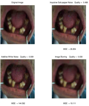
Original Image Impulsive Salt-pepper Noise Quality = 0.498
MSE = 26.854
Multiplicative Speckle Noise Quality = 0.060
MSE = 26.900
Additive White Noise Quality = 0.009
MSE = 144.592
Image Blurring Quality = 0.030
MSE = 19.111
Figure 6: Denture images with various type of distortion
Type of distortion MSE Quality measure (Q)
Impulsive salt-pepper noise 26.854 0.498
Additive white Gaussian noise 144.592 0.009
Multiplicative speckle noise 26.900 0.060
Blurring 19.111 0.030
0 50 100 150 200 250 300
0.002 0.004 0.006 0.008 0.009
MS
E
Noise Degradation
Graph 1: Result of "Lena" images with
various types of distortion.
0 50 100 150 200
0.004 0.006 0.008
MS
E
Noise Degradation
Graph 2:Results of denture images with
various types of distortion
Most human observers would agree with the rankings given by the proposed quality measure and in that sense these results are very reasonable.
4. Conclusion
An algorithm for image quality assessment has been described. The algorithm uses a simple HVS model, which is used to process input images. CSF used in this model is not fixed; it has one user-defined parameter, which controls attenuation at high frequencies. This way it is possible to get better results than in the case when CSF with fixed parameters is used. Finally, image quality measure is computed as the average correlation coefficient between two input images modified by the average correlation coefficient between original image and error image. This way we differentiate between random and signal dependant distortion, which have different impact on a human observer. The results presented here are obtained for the following parameters: viewing distance 60 cm, width of images 15 cm, height of images 15 cm and all images are 512x512 pixels. The future work on this is to develop algorithm to enhance the medical images quality.
5. References
[1] Berlin.(2008): How to measure image quality in tissue-based diagnosis (diagnostic surgical pathology), VSV Interdisciplinary Medical Publishing Mol Med, pp.121-43.
[2] Claypool, Morgan(2007): Modern Image Quality Assessment, IJIST(18), 2, pp. 94-100.
[4] Damera-Venkata, N. , et al. (2000): Image quality assessment based on a degradation model, IEEE Transaction on Image Processing, 9(4), pp. 630-650.
[5] Lim, J. S.(1990): Two-dimensional signal and image processing, Prentice-Hall, Englewood Cliffs, New Jersey.
[6] Mannos J. L. ; Sakrison, D. J.(1974): The effects of a visual fidelity criterion on the encoding of images, IEEE Transactions on Information Theory, 20(4), pp. 525-536.
[7] Pappas, T. N. ; Michel, T. A.; Hinds, R. O.(1996): Supra-threshold perceptual image coding, in Proc. International Conf. on Image Processing (ICIP), 1, pp. 237-240.
[8] Pappas, T. N. ; Neuhoff, D. L.(1999): Least-squares model based halftoning, IEEE Transactions on Image Processing, 8(8), pp. 1102-1116.
[9] Pappas, T. N. ; Safranek, R. J. (2000): Perceptual criteria for image quality evaluation, in Handbook of image and video processing, Academic Press.
[10] Safranek, R. J. ; Johnston, J. D.(1989): A perceptually tuned subband image coder with image dependant quantization and post-quantization data compression, in Proc. International Conference on Acoustics, Speech, and Signal Processing (ICASSP), 3, pp. 1945-1948.
[11] Smeulders, AWM. et al.(2000): Content-based image retrieval at the end of the early years, IEEE Transactions on Pattern Analysis and Machine Intelligence , 22(12),pp. 1349-80.
[12] Wang, Z. ; Bovik , A. C.; Lu, L.(2002): Why is image quality assessment so difficult?, in Proc. International Conference on Acoustics, Speech, and Signal Processing (ICASSP), 4, pp. 3313-3316.