A Study of Generalization and Fitness
Landscapes for Neuroevolution
NUNO M. RODRIGUES 1, (Graduate Student Member, IEEE), SARA SILVA1, AND LEONARDO VANNESCHI1,2
1LASIGE, Departamento de Informática, Faculdade de Ciências, Universidade de Lisboa, 1749-016 Lisboa, Portugal
2NOVA Information Management School (NOVA IMS), Universidade Nova de Lisboa, Campus de Campolide, 1070-312 Lisboa, Portugal
Corresponding author: Nuno M. Rodrigues ([email protected])
This work was supported in part by FCT, Portugal, through funding of LASIGE Research Unit under Grant UIDB/00408/2020 and Grant UIDP/00408/2020, in part by BINDER under Grant PTDC/CCI-INF/29168/2017, in part by GADgET under Grant DSAIPA/DS/0022/2018, in part by AICE under Grant DSAIPA/DS/0113/2019), and in part by PREDICT under Grant PTDC/CCI-CIF/29877/2017.
ABSTRACT Fitness landscapes are a useful concept for studying the dynamics of meta-heuristics. In the last two decades, they have been successfully used for estimating the optimization capabilities of different flavors of evolutionary algorithms, including genetic algorithms and genetic programming. However, so far they have not been used for studying the performance of machine learning algorithms on unseen data, and they have not been applied to studying neuroevolution landscapes. This paper fills these gaps by applying fitness landscapes to neuroevolution, and using this concept to infer useful information about the learning and generalization ability of the machine learning method. For this task, we use a grammar-based approach to generate convolutional neural networks, and we study the dynamics of three different mutations used to evolve them. To characterize fitness landscapes, we study autocorrelation, entropic measure of ruggedness, and fitness clouds. Also, we propose the use of two additional evaluation measures: density clouds and overfitting measure. The results show that these measures are appropriate for estimating both the learning and the generalization ability of the considered neuroevolution configurations.
INDEX TERMS Autocorrelation, convolutional neural networks, density clouds, entropic measure of
ruggedness, fitness clouds, fitness landscapes, generalization, neuroevolution, overfitting.
I. INTRODUCTION
The concept of fitness landscapes (FLs) [1], [2] has been used many times to characterize the dynamics of meta-heuristics in optimization tasks. Particularly, several measures have been developed with the goal of capturing essential characteristics of FLs that can provide useful information regarding the diffi-culty of different optimization problems. Among these mea-sures, autocorrelation [3], fitness clouds [4], [5], and entropic measure of ruggedness (EMR) [6]–[8] have been intensively studied, revealing to be useful indicators of the ruggedness and difficulty of the FLs induced by several variants of local search meta-heuristics and evolutionary algorithms (EAs) [9]. However, to the best of our knowledge, despite existing few works on Fls where measures such as EMR, Fitness Distance Correlation and gradient analysis were applied to standard neural networks [10], [11], no measure related to FLs has ever The associate editor coordinating the review of this manuscript and approving it for publication was F. K. Wang .
been used for studying the performance of machine learn-ing (ML) algorithms on unseen data, nor for characterizlearn-ing the dynamics of neuroevolution. In this work, we adapt the well-known definitions of autocorrelation, fitness clouds and EMR to neuroevolution. We also use two other measures, density clouds and overfitting measure, not only to study the optimization effectiveness of various neuroevolution config-urations, but also to characterize their performance on unseen data. We also introduce our own grammar-based neuroevolu-tion approach, inspired by existing systems.
Neuroevolution is a branch of evolutionary computation that has been around for almost three decades, with appli-cation in multiple areas such as supervised classifiappli-cation tasks [12] and agent building [13]. In neuroevolution, an EA is used to evolve weights, topologies and/or hyper-parameters of artificial neural networks. In this study, we focus on the evolution of convolutional neural networks (CNNs), because they are one of the most popular deep neural network architectures with applications including computer
vision [14], [15], gestures recognition [16] and activity recog-nition [17]. They have a vast amount of tunable parameters that are difficult to set, which makes them perfect for testing the capabilities of neuroevolution. For testing the reliability of the studied measures in predicting the performance of neuroevolution of CNNs on training and unseen data, we con-sider three different types of mutations and four different multiclass classification problems, with different degrees of known difficulty. For each type of mutation, and for each one of the studied problems, we calculate the value of these mea-sures and we compare them to the results obtained by actual simulations performed with our neuroevolution system.
We consider this work as the first proof of concept in a wider study, aimed at establishing the use of measures to characterize neuroevolution of CNNs. If successful, this study will be extremely impactful. CNNs normally have a slow learning phase, which makes neuroevolution a very intensive computational process, as it requires the evaluation of several CNNs in each generation. For this reason, the task of executing simulations to choose among different types of genetic operators, and/or among several possible parameter settings, is normally prohibitively expensive. This may result on the adoption of sub-optimal configurations that not only will require a tremendous amount of training time due to learning difficulty, but also will perform sub-optimally after training because of poor generalization ability. On the other hand, the calculation of the studied measures is much faster, and therefore it can help us find appropriate neuroevolu-tion configuraneuroevolu-tions much more efficiently, with one such example being presented in section IV-B1. The end result may be that the time spent on calculating the measures will be largely compensated with optimized configurations that will learn faster and generalize better. Computational con-straints have also prompted us to choose simple measures that are both quick to calculate and, as our results demonstrate, effective.
The paper is organized as follows: in SectionII, we intro-duce the concept of FL and the used measures. SectionIII
introduces neuroevolution and presents our grammar-based approach to evolve CNNs. In Section IV, we present our experimental study, first discussing the test problems used, then the experimental settings, and finally presenting and discussing the obtained results. Finally, SectionVconcludes the paper and suggests ideas for future research.
Public repository for reproducibility: https://github.com/NMVRodrigues/TFNE II. FITNESS LANDSCAPES
Using a landscape metaphor to gain insight about the work-ings of a complex system originates with the work of Wright on genetics [1]. Probably, the simplest definition of FL is the following one: a FL can be seen as a plot where the points in the horizontal direction represent the different individual genotypes in a search space and the points in the vertical direction represent the fitness of each one of these individ-uals [18]. If genotypes can be visualized in two dimensions,
the plot can be seen as a three-dimensional ‘‘map’’, which may contain peaks and valleys. The task of finding the best solution to the problem is equivalent to finding the highest peak (for maximization problems) or the lowest valley (for minimization). The problem solver is seen as a short-sighted explorer searching for those optimal spots. Crucial to the concept of FL is that solutions should be arranged in a way that is consistent with a given neighborhood relationship. Indeed, a FL is completely defined by the triple:
(S, f , N)
where S is the set of all admissible solutions (the search space), f is the fitness function, a function used to measure the quality of the solutions found by the algorithm, and, N is the neighborhood. Generally, the neighborhood should have a relationship with the transformation (mutation) operator used to explore the search space. A typical example is to consider as neighbors two solutions a and b if and only if b can be obtained by applying mutation to a.
The FL metaphor can be helpful for understanding the difficulty of a problem, i.e., the ability of a searcher to find the optimal solution for that problem. However, in practical situations, FLs are impossible to visualize, both because of the vast size of the search space and because of the multi-dimensionality of the neighborhood. For this reason, researchers have introduced a set of mathematical measures, able to capture some characteristics of FLs and express them with single numbers [19]. Although none of these measures is capable of expressing completely the vast amount of information that characterizes a FL, some of them revealed to be reliable indicators of the difficulty of problems, for instance: autocorrelation [3], entropic measure of rugged-ness (EMR) [6]–[8], density of states [20], fitrugged-ness-distance correlation [19], [21], length of adaptive walks [2], and basins of attraction size [22], plus various measures based on the concepts of fitness clouds [19] and local optima networks [23].
Among the previously mentioned measures, in this paper we investigate autocorrelation, EMR, and fitness clouds, for two related reasons. Firstly, they are the simplest mea-sures available which, for a very first study on this subject, makes them the most appropriate first choice. If these simple measures were to fail their purpose, we would have used more complex ones. Secondly, they can be quicky calculated, which for a computationally intensive method such as neu-roevolution of CNNs, is an important advantage. Other mea-sures could be so computationally demanding as to render the study of fitness landscapes unfeasible for neuroevolution. Additionally, we introduce a new measure that is an alter-native to the density of states, called density clouds, and we also use a measure of overfitting [24] to analyze the results. Both of these are also simple and easily calculated. All these measures are defined and discussed in the remainder of this section, including how their respective results will be reported later in the experimental section.
A. AUTOCORRELATION
The autocorrelation coefficient is used to measure the rugged-ness of a FL [3]. In the context of Fitrugged-ness Landscapes, the ruggedness of a landscape is related to the amount of present elements, such as hills, slopes and plateaus, and gives and indication of the difficulty of the problem. It is applied over a series of fitness values, determined by a walk on the landscape. A walk on a FL is a sequence of solutions (s0, s1, . . . , sn) such that, for each t = 1, 2, . . . , n, st is a
neighbor of st−1or, in other words, stis obtained by applying
a mutation to st−1. For walks of a finite length n, autocorre-lation with step k is defined as:
ˆ ρ(k) = Pn−k t=1(f (st) − ¯f)(f (st+k) − ¯f) q Pn t=1(f (st) − ¯f)2 q Pn t=1(f (st+k) − ¯f)2 , where ¯f = 1nPn t=1f(st).
Given the huge size of the search space created by neu-roevolution, and in the attempt to generate walks that are, as much as possible, representatives of the portions of the search space actually explored by the evolutionary algorithm, in this work we calculate autocorrelation using selective walks[19]. In selective walks, for each t = 1, 2, . . . , n, st is
a selected solution from the neighborhood of st−1. To apply selection pressure to the neighbors, tournament selection is used; in other words, stis the best solution (i.e., the one with
the best fitness on the training set) in a sample of m randomly generated neighbors of st−1.
We study the autocorrelation both on the training and on the test set, by using the same selective walk. In both cases, selection acts using only training data, but in the former case the individuals are evaluated on the training set, while in the latter case they are evaluated on the test set. Because of the large complexity of neuroevolution, and given the relatively short length of the walks that we are able to generate with the available computational resources1 (n = 30 in our experiments), we calculate ˆρ(k) several times (10 in our experiments), using independent selective walks, and report boxplots of the results obtained over these different walks.
In order to broadly classify the ruggedness of the land-scape, we adopt the heuristic threshold suggested by Jones for fitness-distance correlation [21], where ˆρ(k) > 0.15 corresponds to a smooth landscape (and thus, in principle, an easy problem), and ˆρ(k) < 0.15 corresponds to a rugged hard landscape. To visualize the results, the threshold will be shown as a horizontal line in the same diagram as the boxplots of the autocorrelation, and the position of the box compared to the threshold will allow us to classify problems as easy or hard. The situation in which the boxplot lays across the threshold (i.e., the case in which ˆρ(k) ≈ 0.15) will be considered as an uncertain case, in which predicting the hardness of the problem is a difficult task. One of the typical situations in which we have an uncertain case is when sev-eral different neuroevolution runs yield significantly different
1 Our experiments were performed on a machine with a gtx 970, a gtx 2070 and 16GB of RAM.
results (for instance, half of the runs converge towards good quality solutions and the other half stagnate in bad quality ones). Finally, several values of the step k are compared (k = 1, 2, 3, 4 in our experiments).
B. ENTROPIC MEASURE OF RUGGEDNESS
The EMR is an indicator of the relationship between rugged-ness and neutrality. In the context of Fitrugged-ness Landscapes, we define neutrality, or neutral degree, as the capacity of the algorithm to generate solutions with different fitness values. If multiple solutions have different neighbors with the same fitness, the landscape is deemed to have a high degree of neutrality. It was introduced by Vassilev [6]–[8] and is defined as follows: assuming that a walk of length n, performed on a landscape, generates a time series of fitness values {ft}nt=0, that time series can be represented as a string S(ε) =
{x1x2. . . xn}, where, for each i = 1, 2, . . . , n, xi ∈ { ¯1, 0, 1}.
For each i = 1, 2, . . . , n, xi ∈ S(ε) is obtained using the
following function: xi=9ft(i, ε) = ¯ 1, if fi− fi−1< −ε 0, if |fi− fi−1| ≤ −ε 1, if fi− fi−1> −ε
whereε is a real number that determines the accuracy of the calculation of S(ε), and increasing this value results in increasing the neutrality of the landscape. The smallest pos-sible ε for which the landscape becomes flat is called the information stability, and is represented byε∗. Using S(ε), the EMR is defined as follows [6]:
H(ε) = −X
p6=q
P[pq]log6 P[pq],
where p and q are elements from the set {¯1, 0, 1}, and P[pq]=n[pq]n , where n[pq] is the number of pq sub-blocks in S(ε) and n is the total number of sub-blocks. The output of H (ε) is a value in the [0, 1] range, and it represents an estimate of the variety of fitness values in the walk, with a higher value meaning a larger variety and thus a more rugged landscape. In this definition, for each walk that is performed, H (ε) is calculated for multiple ε values, usu-ally {0, ε∗/128, ε∗/64, ε∗/32, ε∗/16, ε∗/8, ε∗/4, ε∗/2, ε∗}, and then the mean of H (ε), represented as ¯H(ε), over all performed walks is calculated for each value ofε. In this work, we employ the adaptations suggested by Malan [25], aimed at reducing the characterization of the landscape to a single scalar. To characterise the ruggedness of a function f , the following value is proposed:
Rf = max ∀ε∈[0,ε∗]H(ε)
To approximate the theoretical value of Rf, the maximum
of ¯H(ε) is calculated for all ε values.
C. FITNESS CLOUDS
Fitness clouds [4] consist of a scatterplot that maps the fit-ness of a sample of individuals against the fitfit-ness of their
neighbors, obtained by the application of a genetic operator. The shape of this scatterplot can provide an indication of the evolvability of the genetic operators used, and thus offers some hints about the difficulty of the problem. Using the loss as fitness, a plot where most points fall below (above) the identity line is considered to be easy (difficult), as most genetic operators generate individuals that are better (worse) than their parents. Comparing the shape of the plots obtained for the training set and for the test set, it is also possible to obtain an indication regarding the difficulty of generalization on unseen data as models that fail to generalize will produce a test cloud much more concentrated in lower fitness values. Considering a set of individuals S = {s1, s2, . . . , sn},
for each i = 1, 2, . . . , n, a set of neighbors of each indi-vidual si, V(si) = {vi1, vi2, . . . , vimi}and a fitness function f ,
the set of points that form the fitness cloud can be defined as follows:
C = {(f (si), f (vik)), ∀i ∈ [1, n], ∀k ∈ [1, mi]} (1)
As explained by [26], fitness clouds also implicitly provide information about the genotype to phenotype mapping. The set of genotypes that have the same fitness is called a neutral set [27], which can be represented by one abscissa in the fitness/fitness plane. According to this abscissa, a vertical slice from the cloud represents the set of fitness values that could be reached from this set of neutrality. For a given offspring fitness value f , an horizontal slice represents all the fitness values from which one can reach f .
D. DENSITY CLOUDS
We propose the use of a new measure called density clouds as an alternative to the density of states. Density clouds allows us to use the same sample that is used for fitness clouds, whereas density of states would require a much larger sample, since we would need to find neighbours in that sample, a very hard task in such a large space of possibilities. Density clouds uses the same points as the fitness clouds to produce a visual representation of the shape and density of that distribution. The visual interpretation of density clouds is essentially the same as for fitness clouds, but concentrated on the areas with the largest density of points, with the added advantage that the plots will still be easily interpretable in a space of thousands of samples.
Let {X1, X2, . . . , Xn}be a univariate independent and
iden-tically distributed sample drawn from some distribution with an unknown density f . The kernel density estimator is:
ˆ fh(x) = 1 nh n X i=1 K(x − xi h ), (2)
where K is a kernel function and h is the bandwidth.
E. SAMPLING METHODOLOGY
Many of the previously discussed measures can be calculated using a sample of the search space. However, as discussed in [19], the sampling methodology used to generate this set
of individuals may be crucial in determining the usefulness of the measures. As in [19], also in this work we use a Metropolis-Hastings [28] approach. Similarly to selective walks, this methodology has a selection pressure. This char-acteristic makes Metropolis-Hastings sampling preferable compared to a simple uniform random sampling. Particularly in our study, given the huge size of the neuroevolution search space, uniform random sampling is unlikely to generate a sample that may represent the search space portion actually explored by the EA. A good example is a plateau: with uni-form random sampling, multiple points with the same fitness could be re-sampled, while using Metropolis-Hastings, only one point would be sampled and then the algorithm would look for better solutions. Since neuroevolution works with loss values that are unbounded, we have performed some changes on the Metropolis-Hastings algorithm, compared to the version used in [19]. The method we use is described in Algorithm1.
Algorithm 1 Metropolis-Hastings Sampling
1 Sample size = n
2 Generate a random individual x1 3 for t = 1,2,. . . ,n do
4 Generate a random candidate individual x0 5 Calculate the acceptance ratioα = norm(x
0 ) norm(xt) 6 ifα ≥ u ∈ σ(0, 1) then
7 Accept the candidate, xt+1= x0 8 else
9 Reject the candidate, xt+1= xt
We normalize the fitness values using the following expression: norm(x) =1+f (x)1 , where f (x) is the fitness of the individual x. This normalization is done since we are working with loss values in the range [0, ∞].
F. OVERFITTING DETECTION
In [24], Vanneschi et al. proposed a measure to quantify overfitting during the evolution of GP algorithms. We propose using this measure with slight modifications and apply it to selective walks in order to predict the generalization ability of the models. Algorithm2describes the measure, that will be called OverFitting Measure (OFM) from now on. Intuitively, the amount of overfitting measured at a given moment is based on the difference between training and test fitness, and how much this difference has increased since the best test point (btp), i.e., the moment in which the test fitness was at its best (lines 12–14). The btp is set at the beginning of the walk, with overfitting being 0 at that moment (lines 2–3). Every time a new best test fitness is found, the btp is updated to that point of the walk, and overfitting is again set to 0 (lines 8–10). Overfitting is also set to 0 when the training fitness is worse than the test fitness (lines 5–6). Because the selective walk does not use elitism, we are bounding the amount of
Algorithm 2 Method Used to Measure Overfitting
1 Length of the walk = n 2 Best test point, btp = 0 3 overfit(btp) = 0 4 for i = 1,2,. . . ,n do
5 if training_fit(i)> test_fit(i) then
6 overfit(i) = 0
7 else
8 if test_fit(i)< test_fit(btp) then
9 btp = i
10 overfit(btp) = 0
11 else
12 diff_now = |training_fit(i)−test_fit(i)| 13 diff_btp = |training_fit(btp)−test_fit(btp)|
14 overfit(i) = max(0, diff_now−diff_btp)
overfitting to 0, otherwise it would be possible to arrive at negative values (max at line 14).
III. NEUROEVOLUTION
Neuroevolution is usually employed to evolve the topology, weights, parameters and/or learning strategies of artificial neural networks. Some of the most well known neuroevolu-tion systems include EPNet [29], NEAT [13], EANT [30], and hyperNEAT [31]. Most recently, works have appeared that apply neuroevolution to other types of neural networks, such as CNNs [32]–[34]. In this section we describe how we represent networks using a grammar-based approach, and we discuss the employed genetic operations.
A. GRAMMAR-BASED NEUROEVOLUTION
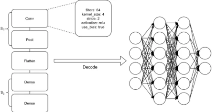
We have decided on a grammar-based approach because of its modularity and flexibility. The grammar we have developed is based on existing systems, and it is reported in Fig. 1. It contains all the possible values for the parameters of each available layer. This way, adding and removing types of layers or changing their parameters is simple and requires minimal changes. Using this grammar, we are discretizing the range of the possible values that each parameter can take. This greatly reduces the search space, while keeping the quality of the solutions under control, as in most cases, intermediate values can have little to no significant influence on the effectiveness of the solutions, as reported in [12].
1) GENOTYPE ENCODING
In our representation, genotypes are composed by two dif-ferent sections, S1 and S2, that are connected using the so called Flatten gene. The Flatten gene implements the con-version (i.e., the ‘‘flattening’’) of multidimensional feature matrices from the convolutional layers into a one dimensional array that is fed to the following fully connected layer. On S1 we have genes that encode the layers that deal with feature
FIGURE 1. Grammar used to evolve CNNs.
extraction from the images, convolutional and pooling layers, and on S2 we have genes that encode the classification and pruning parts of the network, dense and dropout layers. Separating the network into these two segments helps make the implementation more modular and expandable, provided that when adding or removing new layers will only affect interactions within their segment. Besides the flatten layer, the only other layer that is the same for all possible individuals is the output layer, which is a fully connected (i.e., dense) layer with softmax activation and a number of units equal to the number of classes to be predicted. The genetic operators cannot modify this layer, except for the bias parameter. Before evaluation, a genotype is mapped into a pheno-type (Fig.2), that is a neural network itself, and all weights are initialized following the Glorot initialization method [35].
FIGURE 2. Example of a genome built by the grammar and the network it produces when decoded.
2) GENETIC OPERATORS
Due to the difficulty of defining a crossover-based neigh-borhood for studying FLs [36], we consider only mutation operators. Given the vast amount of mutation choices in neuroevolution, we restrict our study to three different types of operators:
• Topological mutations: Mutations that add or delete a gene, except for the flatten gene, changing the topol-ogy of the genotype and, consequently, the one of the phenotype.
• Parameter mutations: Mutations that change the parameters encoded in a gene. They cover all parameters of all gene types, excluding the flatten gene (which has no parameters).
• Learning mutations: Mutations that change the Optimizer’s parameters that guide the learning of the networks. These parameters are encoded in the Optimizer gene (see Fig.1).
3) EVALUATION
Evaluation involves training the network and calculating its performance on the given data. During the evolutionary pro-cess, we use the loss value on the training set as a fitness function to evaluate the networks. Regarding the optimizer used for training the networks, we have chosen Stochastic Gradient Descent (SGD) over ADAM [37] due to two impor-tant factors: the range of values for the SGD parameters has been extensively tested, so the value choice could be done more accurately; although ADAM is more common nowa-days due to achieving better overall results, SGD outperforms ADAM when it comes to generalization ability [38]. Also, since we are working with multiclass classification problems that are not one-hot encoded, we used Sparse Categorical Cross-Entropy as a loss function, which motivates the need to have the fixed number of neurons and activation function in the output layer. To evaluate the generalization ability of the individuals, we also measure the accuracy and loss in a separate test set.
IV. EXPERIMENTAL STUDY
A. DATASETS AND EXPERIMENTAL SETTINGS
Table1describes the main characteristics of the datasets used as test cases in our experiments. The partition into training and test set is made randomly, and it is different at each run. For all datasets,2a simple image scale adjustment was done, setting pixel values in the [0, 1] range. No further data pre-processing or image augmentation was applied to the datasets. The MNIST dataset consists in a set of gray scale images of handwritten digits from 0 to 9 [39]. Fashion-MNIST (FMNIST) is similar to MNIST, but instead of having digits from 0 to 9, it contains images of 10 differ-ent types of clothing articles [40]. CIFAR10 contains RGB pictures of 10 different types of real world objects [41]. SVHN contains RGB pictures of house numbers, containing digits from 0 to 9 [42]. SM (small and mislabelled) is a
2all of the datasets are public and freely available
TABLE 1. Number of training and test observations, and number of classes of each dataset.
hand-tailored dataset that we have artificially created to have a case in which neuroevolution clearly overfits. It was created by taking the last 30% of samples from MNIST and chang-ing half of the values from each odd label to another label (more specifically, label 1 was changed into a 3, 3 became 9, 5 became 0, 7 became 4, and 9 became 1).
All of the previously mentioned datasets, besides SM, are public and freely available. For each one of these datasets and for each one of the three studied mutation operators, we perform sampling using the Metropolis-Hastings method (for all the measures related to, and including, fitness clouds), selective walks (that allow us to have all the needed infor-mation to calculate the autocorrelation and the EMR) and we execute the neuroevolution. From now on, we will use the term configuration to indicate an experiment in which a particular type of mutation was used on a particular dataset. For each configuration, we generate a sample of 500 indi-viduals using Metropolis-Hastings, 10 independent selective walks and 10 independent neuroevolution runs. All neuroevo-lution runs are performed starting with a randomly initialized population of individuals, and all the selective walks are constructed starting with a randomly generated individual.
To determine the values of the main parameters (e.g., pop-ulation size and number of generations for neuroevolution, length of the walk and number of neighbors for selective walks, etc.) we have performed a preliminary experimental study with multiple values, and selected the ones that allowed us to obtain results in ‘‘reasonable’’ time3with our available computational resources.1However, we do acknowledge that as with any evolutionary algorithm, higher values for these parameters produce stronger and more accurate results.
The employed parameter values are reported in Table2. The first column contains the parameters used to perform the selective walks and sampling, while the second column contains the parameters of the neuroevolution. One should keep in mind that, in order to evaluate all the neural networks in the population, all the networks need to go through a learning phase at each generation of the evolutionary process. The third column reports the values used by each one of those networks for learning.
TABLE 2.Parameter values used in our experiments.
B. EXPERIMENTAL RESULTS
We now describe the results obtained in our experiments. We analyse the predictive value of the different measures we use to characterize fitness landscapes, observing the results
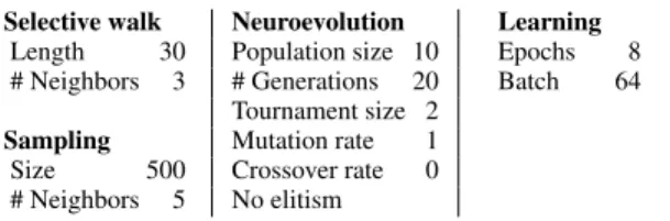
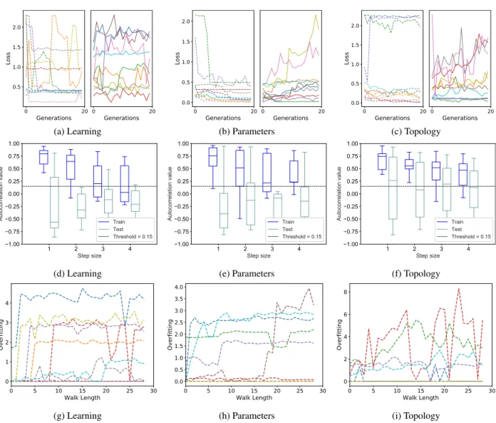
FIGURE 3. MNIST dataset. Plots (a), (b) and (c): neuroevolution results; plots (d), (e) and (f): autocorrelation results; plots (g), (h) and (i): results of the measure of overfitting (OFM). Plots (a), (d) and (g): results for the learning mutation; plots (b), (e) and (h) for the parameters mutation; plots (c), (f) and (i) for the topology mutation. Remarks: plots (a), (b) and (c) report the evolution of the best fitness in the population at each generation (one curve for each performed neuroevolution run). Each plot is partitioned into two subfigures: training loss on the left and test loss on the right. Plots (d), (e) and (f) report the boxplots of the autocorrelation, calculated over 10 independent selective walks. Plots (g), (h) and (i) report the evolution of the OFM value for each of the 10 independent selective walks.
obtained in each problem, and then we briefly comment on the general performance of the different types of mutation used.
1) AUTOCORRELATION AND OVERFITTING MEASURE
We begin by analyzing the ability of autocorrelation to characterize training and test performance of neuroevolu-tion of CNNs, as well as the ability of OFM to detect and measure overfitting. Fig.3reports the evolution of the loss, the autocorrelation and the OFM for the MNIST problem. The first line of plots reports the evolution of the loss against generations for the three studied mutation operators. Each plot in the first line is partitioned into two halves: the leftmost one reports the evolution of the training loss of the best individual, while the rightmost one reports the loss of the same individual, evaluated on the unseen test set. Each curve
in these plots reports the results of one neuroevolution run. The second line contains the boxplots of the autocorrelation values, calculated over 10 independent selective walks, both on the training and on the test set. The third line reports the evolution of the OFM value against the length of a selective walk for each different mutation type. Each curve reports the results of a single walk. Each column of plots reports the results for a different type of mutation, allowing us to easily compare the outcome of the neuroevolution and the one of the studied measures for the different configurations.
As we can observe from plots (a) and (b) of Fig. 3, when we employ learning mutation and parameters mutation, the MNIST problem is easy to solve, both on training and test set. This is confirmed by the fact that 14 out of 20 runs have a loss value below 0.2 which translates in accuracy values ranging from 94% up to 98%. Furthermore, the evolution of
FIGURE 4. FMNIST dataset. The organization of the plots is analogous to Figure3.
the loss suggests that given more generations these values would improve since the majority of the runs was still, slowly, converging towards zero. Now, looking at plots (d) and (e), we observe that the autocorrelation captures the fact that the problem is easy. In fact, in both cases, practically the whole autocorrelation box stands above (and the medians never go below) the 0.15 threshold. When the topology mutation is used, the situation changes: the number of runs in which the evolution does not have a regular trend is larger. This may not be obvious by looking at plot (c), because of the scale of the y-axis, but the lines are now much more rugged than they were for the other two cases. The problem is now harder than it was, and as we can see in plot (f), the autocorrelation catches this difficulty. In particular, we can observe that when the step is equal to 4, the whole autocorrelation boxes are below the threshold. Finally, looking at plots (g) to (i), we observe that OFM captures the fact that neuroevolution does not overfit for the MNIST dataset. In fact, the OFM values are always low, and keep returning to 0.
The partial conclusion that we can draw for the MNIST dataset is that learning and parameter mutations are more effective operators than topology mutations, and this is cor-rectly predicted by the autocorrelation. Furthermore, we can observe that the neuroevolution results obtained on the test set are very similar to the ones on the training set, practically for all the runs we have performed. Also this feature is captured by the autocorrelation, since the training and test boxes are very similar to each other for practically all the configurations. This is an indication of lack of overfitting, and this feature is correctly measured by the OFM.
Now we consider the results obtained for the FMNIST dataset, reported in Fig. 4. Describing the results for this dataset is straightforward: observing the neuroevolution plots, we can see that for the three configurations the problem is easy, both on training and test set. In fact, all the curves are steadily decreasing and/or close to zero. For the learning operator, all runs ended with loss values below 0.5, which translates in accuracy values ranging from 85% up to 92%.
FIGURE 5. CIFAR10 dataset. The organization of the plots is analogous to Figure3.
For both parameter and topology operators, a total of 12 out of 20 runs report loss values under 0.5. Observing the scale on the left part of the plots, we can also observe that when topol-ogy mutation is used (plot (c)), the problem is slightly harder than when the other mutations are used, since the achieved values of the loss are generally higher. All this is correctly measured by the autocorrelation, given that the boxes are above the threshold for all the configurations, and, in the case of the topology mutation (plot (f)), they are slightly lower than in the other cases. Last but not least, also in this case training and test evolution of loss are very similar between each other, and this fact finds a precise correspondence in the autocorrelation results, given that the training boxes are generally very similar to the test boxes. This also indicates no overfitting, and this fact is correctly captured by the OFM, that shows values that keep returning to 0. All in all, we can conclude that also for the FMNIST dataset, autocorrelation is a reliable indicator of problem hardness and the OFM correctly predicts lack of overfitting.
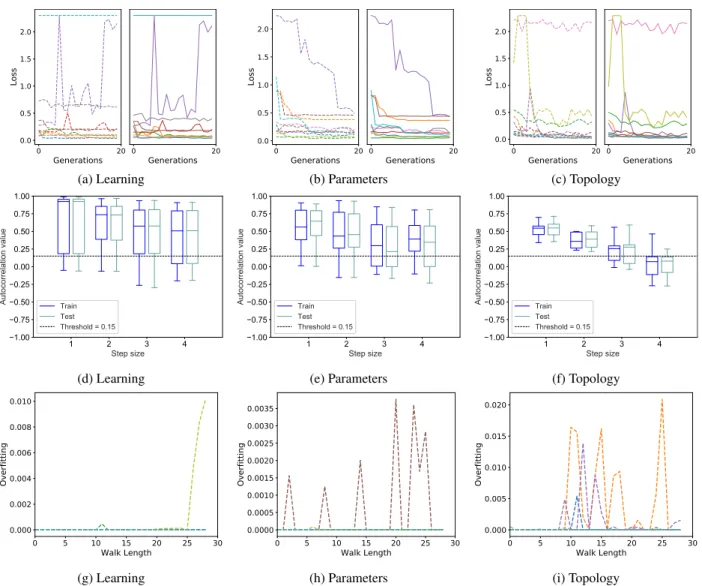
The results for the CIFAR10 dataset are reported in Fig.5. Observing the neuroevolution results, we can say that when the learning mutation is used, the problem is substantially easy (almost all the loss curves have a smooth decreasing trend); however, at the same time, among the three types of mutation, learning mutation is the one in which there is a more marked difference between training and test evolution, which indicates the possibility of overfitting, at least in some runs. Interestingly, on the learning operator, in the training plot only half of the runs present loss below 0.5, but in the test plot, despite the clear overfitting, we have six runs below that threshold, one more than in training. At the same time, when the parameters mutation is used, the problem is uncertain (in some runs the loss curves have a decreasing trend, while in others they have an increasing trend), but the training and test evolution are rather similar between each other in every run. For this operator, loss values are in the range of [1, 2.3], which translates into accuracy values in the range of [62%, 10%]. Finally, when the topology mutation is used, the problem is
FIGURE 6. SVHN dataset. The organization of the plots is analogous to Figure3.
hard (almost all the loss curves have an increasing trend), but once again no substantial difference between training and test behaviors can be observed. This operator produced loss values highly similar to the ones produced by the parameters mutation, with only a slight change in the lower bound. Loss values are in the range of [1.3, 2.3], which translates into accuracy values in the range of [63%, 10&]. Looking at the autocorrelation results, we find a reasonable correspondence: for the learning mutation all the boxes are clearly above the threshold, for the parameters mutation the boxes are not as high as for the learning mutation, beginning to cross the threshold with steps 3 and 4, and finally for the topology mutation the boxes are even lower, with the medians below the threshold for steps 3 and 4, and more than half the height of the boxes also below the threshold for step 4. As already observed in plot (f) of Fig. 4, longer steps seem to be better indicators, when the autocorrelation is applied to hard problems. The different behavior between training and test set also finds a correspondence in the autocorrelation
results (plot (d)), given that the test boxes are taller than the training boxes, in particular for step 4. At the same time, the potential presence of overfitting is clearly detected by the OFM (plot (g)), that assumes growing values in some cases. As for plots (h) and (i), they reflect absence of over-fitting for parameters and topology mutations, as expected. All in all, also for the CIFAR10 dataset the autocorrelation is a reasonable indicator of problem difficulty, while the OFM reveals to be a good measure of overfitting.
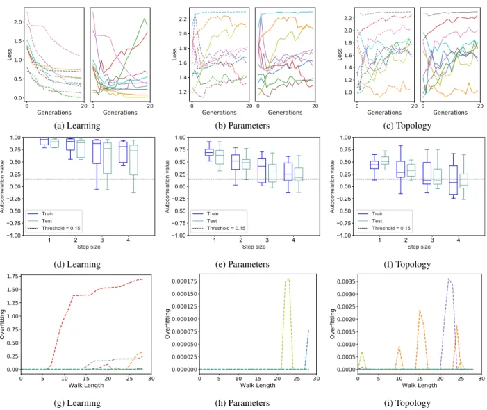
The results for the SVHN dataset are reported in Figure6. In this case, the plots of the loss evolution indicate that the problem is uncertain when learning mutation is used (given that approximately half of the curves have a decreasing trend, while the other half have an oscillating trend), easy when parameters mutation is used (with the majority of the curves having a decreasing trend) and hard when topology mutation is used (with most curves exhibiting an oscilla-tory behaviour, which indicates poor optimization ability). On the learning operator we have loss values in the range
FIGURE 7. SM dataset. The organization of the plots is analogous to Figure3.
of [0.56, 2.23], which translates into accuracy values in the range of [84%, 19%], and only four runs ended with a loss value below 1.0. Both parameter and topology operators have very close boundary values, both having all runs in the range of [0.23, 2.23] loss wise and [93%, 19%] accuracy wise, with only three runs below 1.0 loss each.
At the same time, some differences, although minimal, can be observed between training and test evolution. Specifically, when a run has an oscillatory behavior, the oscillations tend to be larger on the test set than on the training set (for instance, but not only, in the dark blue curves on plot (a), the violet curves in plot (b) and the red curves in plot (c)). Also in this case, autocorrelation is confirmed as a reasonable indicator of problem difficulty. In fact, for learning mutation, the boxes are crossing the threshold for steps 3 and 4, for parameters mutation they are above the threshold, and for topology mutation they are almost completely below the threshold for steps 3 and 4. The medians are lower and the dispersion of values is larger for step 4, which reflects well
the neuroevolution behavior observed in plot (c) (unstable and often returning to high values of the loss). The highest step size is once again the most reliable. Regarding OFM, it reveals several peaks but no clear trend, either because there is no overfitting or because both training and test fitness values oscillate too much to reveal a trend.
There was also an interesting finding regarding the topol-ogy of the best network obtained by the topoltopol-ogy operator. Earlier in sectionIwe claimed that FL analysis of neuroevo-lution could help find configurations better and faster than manually tailored ones. The previously mentioned solution serves as an example of such, where a network composed only by six different size convolutional layer and two small dense layers can outperform solutions with more common topologies that include pooling and dropout layers.
Finally, we analyse the results obtained on the SM dataset, reported in Figure 7. Looking at plots (a), (b) and (c), we can observe the following facts: first of all, neuroevolution overfits in all the three cases. This was expected, since the
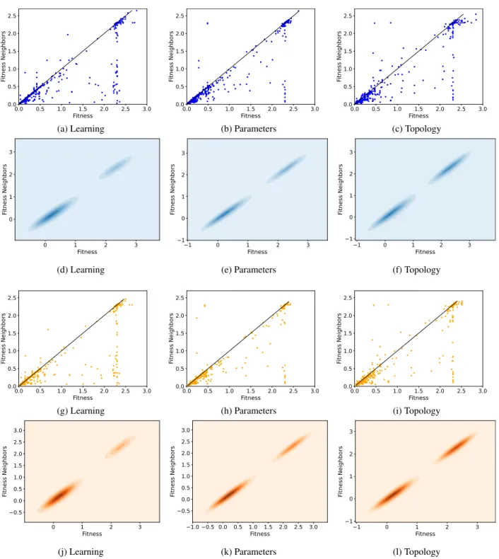
FIGURE 8. MNIST dataset. Plots (a), (b), (c), (g), (h), and (i): fitness clouds; plots (d), (e), (f), (j), (k), and (l): density clouds. Plots (a) to (f) refer to the training set; plots (g) to (l) refer to the test set.
SM dataset was explicitly created with the objective of having a test case with substantial overfitting, and can be observed looking at the large differences between training and test evolution. In particular, we can see that in some cases the loss curves are steadily decreasing on the training set, while they are either increasing or oscillating on the test set. Secondly, we observe that, for the SM dataset, evolution is harder when using learning mutation, compared to either parameters or
topology mutations. Both these observations find a corre-spondence in the autocorrelation boxplots. In fact, the train-ing and test boxes are visibly different, with the test boxes always positioned lower, and often taller, compared to the training ones. Even more importantly, training boxes are often (completely, or almost completely) above the threshold, while test boxes are always (completely or in large part) below the threshold. At the same time, as we can see in plot (d),
FIGURE 9. FMNIST dataset. The organization of the plots is analogous to Figure8.
for learning mutation and step size equal to 4, the median is lower than the threshold on the training set, and this is the only case in which this event verifies, indicating a bigger difficulty for the learning mutation. Concerning the OFM, it correctly detects the overfitting, producing very high results in all three plots. This again serves as a confirmation that the OFM is able to detect and quantify overfitting. It is also interesting to compare the OFM values for CIFAR10 in the only case where
an overfitting trend was observed (Figure5, plot (g)) and in the SM dataset: OFM values are clearly larger for SM, which correctly indicates the larger amount of overfitting observed.
2) FITNESS CLOUDS AND DENSITY CLOUDS
We now investigate the ability of fitness clouds and density clouds to predict the difficulty of a problem. Also in this
FIGURE 10. CIFAR10 dataset. The organization of the plots is analogous to Figure8.
case, the results will be presented by showing one figure for each test problem. In all these figures, the arrangement of the plots is the same: the first (respectively the third) line of plots contains a visualization of the fitness clouds on the training set (respectively on the test set), and the second (respectively the fourth) line contains density clouds on the training set (respectively on the test set). As in the previous section, each column of plots contains the results for a particular mutation operator. Table3 presents the percentage of points that are
below or coincident with the identity like for each problem in training and test, which helps assess the difficulty of the problems.
We begin by studying the results obtained on the MNIST dataset (Figure8). As we can see in plots (a), (b) and (c), regardless of the chosen operator, on the training set the problem is deemed easy by the fitness clouds, as the vast majority of the points of the fitness clouds are below the identity line.
FIGURE 11. SVHN dataset. The organization of the plots is analogous to Figure8.
These results are confirmed by the density clouds in plots (d) (e) and (f). For all operators, we observe two distinct clusters, both over the identity line, one on good (low) fitness values and the other on bad (high) fitness values. The cluster of highest density is the one closer to the origin, which cor-roborates the fact that the problem is easy. In fact, the majority of solutions generated by the Metropolis-Hastings sampling are good quality solutions. As for the test set, results are very similar to the ones on the training set. The majority of the
points in the fitness clouds are below the identity line, and the highest density clusters in the density clouds are concentrated close the origin. In agreement with the autocorrelation and OFM results discussed previously, fitness clouds and density clouds confirm that neuroevolution has no overfitting for the MNIST dataset.
The results obtained on the FMNIST dataset, reported in Figure9, are identical to the ones of MNIST, with only one small difference concerning the parameters operator: both on
FIGURE 12. SM dataset. The organization of the plots is analogous to Figure8.
the training and on the test set, in the density clouds we can see that both clusters are not completely separate. They are connected since there is a slightly higher density of samples with an average performance.
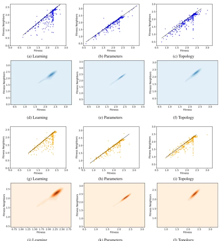
We now study the results obtained on the CIFAR10 dataset, shown in Figure 10. Two different facts can be observed: first of all, in the fitness clouds, the vast majority of the points stands below the identity line; secondly, in the density
clouds only one cluster is visible, and it is located over the identity line but rather far from the origin. Combining these two observations, we can conclude that sampling good solu-tions is hard, even with a sampling method that uses selec-tion pressure like our version of the Metropolis-Hastings. However, the genetic operators are effective, since they are able to improve fitness, often generating better offspring than their parents. Although this is true for all the three studied
FIGURE 13. Results of the Entropic Measure of Ruggedness ¯H(ε) over different values of ε∗for the the three mutation operators on the four considered test problems.
TABLE 3. Table containing the % of points from the fitness clouds either below or coincident with the identity line for each of the problems.
types of mutation, it is particularly prominent in the learning operator, shown as a protuberance in the density clouds.
The results for the SVHN dataset are reported in Figure11. Again, in the fitness clouds the majority of the points are below the identity line, while in the density clouds only one cluster can be observed, and it is rather far from the origin. However, unlike in the previous problems, the points of the fitness clouds exhibit a very low dispersion, being highly concentrated on bad fitness values. Therefore, on one hand we have an indicator of easiness (points below the identity line) while on the other hand we have an indicator of hardness (high density of bad fitness values). SVHN was the dataset where the results of the previous section were rather mixed, and indeed it is difficult to draw conclusions from these plots. The results obtained on the SM dataset are reported in Figure 12. On the training set, we can see that the results are similar to the ones obtained on the MNIST dataset: in the fitness clouds the vast majority of the points are under the identity line, while in the density clouds we have two clusters, the one with the highest density located close to the origin. But the scenario completely changes on the test set, as expected: in the fitness clouds (plots (g), (h) and (i)), the vast majority of the points are located above the identity line, while in the density clouds (plots (j), (k) and (l)) there is only one visible cluster, and it is located rather far from the origin (notice the different scales between training and test). This remarkable difference between training and test set is a further confirmation of the presence of overfitting, as already observed in the previous section.
3) ENTROPIC MEASURE OF RUGGEDNESS
Finally, we study the results of the EMR, reported in Fig.13. Each plot reports the results for one mutation type, showing the values of H (ε) for multiple ε values (see Sect.II-B) on the five studied datasets. These curves illustrate the trend of how ruggedness changes with respect to neutrality. The results show that, overall, the obtained landscapes have a low degree of neutrality, not maintaining the value of H (ε) as ε increases. The most neutral landscape is the one produced by topology mutation on the MNIST dataset (plot (c) of Fig.13). Its highest H (ε) happens when ε = ε∗/64, but the value suffers minimal change fromε = ε∗/128 to ε = ε∗/8.
Table4, which reports the values of Rf for each type of
mutation, and for each studied test problem, corroborates the previous discussion: the maximum value for learning mutation is 0.45, while for parameters mutation is 0.47 and for topology mutation is 0.5. Again, we can see that learning mutations induce the smoothest landscapes, while topology mutations induce the most rugged ones. Also in this case, the prediction of the EMR is compatible with what we observe from the actual neuroevolution runs.
TABLE 4.Rffor each mutation on the studied test problems.
4) CONSIDERATIONS ON MUTATION TYPES
From the three mutation types used in our study, the topology mutation is clearly the worst for both learning and generaliza-tion ability, on all the problems addressed. As for the other two mutation types, while the learning mutation achieves better fitness, it is the parameters mutation that induces the smoothest landscapes. Although some experiments produce a high variability of behaviors, the predictive value of the different measures used to characterize fitness landscapes is maintained for all of the three mutation types.
V. CONCLUSIONS AND FUTURE WORK
Five different measures (autocorrelation, overfitting measure, fitness clouds, density clouds and entropic measure of ruggedness) were used to characterize the performance of neuroevolution of convolutional neural networks for the first time. The results were obtained on five different test prob-lems, and confirm that these measures are reasonable indica-tors of problem hardness, both on the training set and on the test set for the three types of mutation used.
Future work involves the study of other measures of fitness landscapes, on more test problems, with the objective of developing well established, theoretically motivated predic-tive tools for neuroevolution, that can significantly simplify the configuration and tuning phases of the algorithm. We are currently studying the negative slope coefficient [5], [19], in order to quantify the information captured by the fitness clouds with a single number. However, to be calculated in a reliable way, this measure needs larger samples of individu-als. Being able to use more powerful computational archi-tectures, so that we are able to calculate the measures on larger and more significant samples of solutions, is crucial for achieving this and other ambitious goals. Another interesting aspect to confirm is related to the results obtained by the topological mutation. Among the studied operators, in fact, topological mutation was the one that returned the poorest results. If these results are originated from the stacking of layers, we hypothesise that they might be due to the degrada-tion of the training error, as proposed in [43]. To confirm this hypothesis, a thorough analysis of the weights and gradients will be necessary.
REFERENCES
[1] S. Wright, ‘‘The roles of mutation, inbreeding, crossbreeding, and selection in evolution,’’ in Proc. 6th Int. Cong. Genet., vol. 1. Chicago, IL, USA: Univ. of Chicago, 1932.
[2] P. F. Stadler, Fitness Landscapes. Berlin, Germany: Springer, 2002, pp. 183–204.
[3] E. Weinberger, ‘‘Correlated and uncorrelated fitness landscapes and how to tell the difference,’’ Biol. Cybern., vol. 63, no. 5, pp. 325–336, Sep. 1990.
[4] S. Verel, P. Collard, and M. Clergue, ‘‘Where are bottlenecks in NK fitness landscapes?’’ in Proc. Congr. Evol. Comput. (CEC), vol. 1, Dec. 2003, pp. 273–280.
[5] L. Vanneschi, M. Tomassini, P. Collard, and S. Vérel, ‘‘Negative slope coefficient: A measure to characterize genetic programming fitness land-scapes,’’ in Genetic Programming, P. Collet, M. Tomassini, M. Ebner, S. Gustafson, and A. Ekárt, Eds. Berlin, Germany: Springer, 2006, pp. 178–189.
[6] V. K. Vassilev, ‘‘Fitness landscapes and search in the evolutionary design of digital circuits,’’ Ph.D. dissertation, Napier Univ., Edinburgh, U.K., 2000. [7] V. K. Vassilev, T. C. Fogarty, and J. F. Miller, ‘‘Information characteristics and the structure of landscapes,’’ Evol. Comput., vol. 8, no. 1, pp. 31–60, Mar. 2000.
[8] V. K. Vassilev, T. C. Fogarty, and J. F. Miller, ‘‘Smoothness, ruggedness and neutrality of fitness landscapes: From theory to application,’’ in Advances in Evolutionary Computing, A. Ghosh and S. Tsutsui, Eds. Berlin, Germany: Springer, 2003.
[9] S. Vérel, ‘‘Fitness landscapes and graphs: Multimodularity, ruggedness and neutrality,’’ in Proc. Genetic Evol. Comput. Conf. (GECCO), C. Blum and E. Alba, Eds., 2013, pp. 591–616, doi:10.1145/2464576.2480804.
[10] A. Rakitianskaia, E. Bekker, K. M. Malan, and A. Engelbrecht, ‘‘Analysis of error landscapes in multi-layered neural networks for classification,’’ in Proc. IEEE Congr. Evol. Comput. (CEC), Jul. 2016, pp. 5270–5277.
[11] M. Gallagher, ‘‘Fitness distance correlation of neural network error sur-faces: A scalable, continuous optimization problem,’’ in Machine Learn-ing: ECML, L. De Raedt and P. Flach, Eds. Berlin, Germany: Springer, 2001, pp. 157–166.
[12] A. Baldominos, Y. Saez, and P. Isasi, ‘‘Evolutionary convolutional neural networks: An application to handwriting recognition,’’ Neurocomputing, vol. 283, pp. 38–52, Mar. 2018.
[13] K. O. Stanley and R. Miikkulainen, ‘‘Evolving neural networks through augmenting topologies,’’ Evol. Comput., vol. 10, no. 2, pp. 99–127, Jun. 2002.
[14] Y. Guo, Y. Liu, A. Oerlemans, S. Lao, S. Wu, and M. S. Lew, ‘‘Deep learning for visual understanding: A review,’’ Neurocomputing, vol. 187, pp. 27–48, Apr. 2016.
[15] A. Ghazvini, S. N. H. S. Abdullah, and M. Ayob, ‘‘A recent trend in indi-vidual counting approach using deep network,’’ Int. J. Interact. Multimedia Artif. Intell., vol. 5, no. 5, pp. 7–14, 2019.
[16] E. Tsironi, P. Barros, C. Weber, and S. Wermter, ‘‘An analysis of con-volutional long short-term memory recurrent neural networks for gesture recognition,’’ Neurocomputing, vol. 268, pp. 76–86, Dec. 2017. [17] F. Ordóñez and D. Roggen, ‘‘Deep convolutional and LSTM recurrent
neural networks for multimodal wearable activity recognition,’’ Sensors, vol. 16, no. 1, p. 115, Jan. 2016.
[18] W. B. Langdon and R. Poli, Foundations of Genetic Programming. Berlin, Germany: Springer-Verlag, 2002.
[19] L. Vanneschi, ‘‘Theory and practice for efficient genetic programming,’’ Ph.D. dissertation, Fac. Sci., Univ. Lausanne, Lausanne, Switzerland, 2004.
[20] H. Rosé, W. Ebeling, and T. Asselmeyer, ‘‘The density of states—A measure of the difficulty of optimisation problems,’’ in Proc. 4th Int. Conf. Parallel Problem Solving Nature (PPSN). New York, NY, USA: Springer-Verlag, 1996, pp. 208–217.
[21] T. Jones and S. Forrest, Fitness Distance Correlation as a Measure of Problem Difficulty for Genetic Algorithms, L. J. Eshelman, Ed. Burlington, MA, USA: Morgan Kaufmann, 1995, pp. 184–192.
[22] G. Ochoa, S. Verel, and M. Tomassini, ‘‘First-improvement vs. best-improvement local optima networks of NK landscapes,’’ in Parallel Prob-lem Solving From Nature, PPSN XI, R. Schaefer, Ed. Berlin, Germany: Springer, 2010, pp. 104–113.
[23] G. Ochoa, M. Tomassini, S. Vérel, and C. Darabos, ‘‘A study of NK landscapes’ basins and local optima networks,’’ in Proc. 10th Annu. Conf. Genetic Evol. Comput. (GECCO), 2008, pp. 555–562, doi:
10.1145/1389095.1389204.
[24] L. Vanneschi, M. Castelli, and S. Silva, ‘‘Measuring bloat, overfitting and functional complexity in genetic programming,’’ in Proc. 12th Annu. Conf. Genetic Evol. Comput. (GECCO), New York, NY, USA: Association for Computing Machinery, 2010, pp. 877–884.
[25] K. M. Malan and A. P. Engelbrecht, ‘‘Quantifying ruggedness of con-tinuous landscapes using entropy,’’ in Proc. IEEE Congr. Evol. Comput., May 2009, pp. 1440–1447.
[26] L. Vanneschi, M. Clergue, P. Collard, M. Tomassini, and S. Vérel, ‘‘Fitness clouds and problem hardness in genetic programming,’’ in Proc. Genetic Evol. Comput. (GECCO). Berlin, Germany: Springer, 2004, pp. 690–701. [27] M. Kimura, The Neutral Theory of Molecular Evolution. Cambridge, U.K.:
Cambridge Univ. Press, 1983.
[28] N. Madras, Lectures on Monte Carlo Methods (Fields Institute Mono-graphs). Providence, RI, USA: American Mathematical Society, 2002, pp. 2472–4173.
[29] X. Yao and Y. Liu, ‘‘A new evolutionary system for evolving artificial neural networks,’’ IEEE Trans. Neural Netw., vol. 8, no. 3, pp. 694–713, May 1997.
[30] Y. Kassahun and G. Sommer, ‘‘Efficient reinforcement learning through evolutionary acquisition of neural topologies,’’ in Proc. 13th Eur. Symp. Artif. Neural Netw. (ESANN), 2005, pp. 259–266.
[31] K. O. Stanley, D. B. D’Ambrosio, and J. Gauci, ‘‘A hypercube-based encoding for evolving large-scale neural networks,’’ Artif. Life, vol. 15, no. 2, pp. 185–212, Apr. 2009.
[32] P. Verbancsics and J. Harguess, ‘‘Image classification using generative neuro evolution for deep learning,’’ in Proc. IEEE Winter Conf. Appl. Comput. Vis. (WACV). Washington, DC, USA: IEEE Computer Society, Jan. 2015, pp. 488–493.
[33] C. Fernando, D. Banarse, M. Reynolds, F. Besse, D. Pfau, M. Jaderberg, M. Lanctot, and D. Wierstra, ‘‘Convolution by evolution: Differentiable pattern producing networks,’’ in Proc. Genetic Evol. Comput. Conf. (GECCO), 2016, pp. 109–116.
[34] R. Miikkulainen, J. Liang, E. Meyerson, A. Rawal, D. Fink, O. Francon, B. Raju, H. Shahrzad, A. Navruzyan, N. Duffy, and B. Hodjat, ‘‘Evolving deep neural networks,’’ in Artificial Intelligence in the Age of Neural Networks and Brain Computing, R. Kozma, C. Alippi, Y. Choe, and F. C. Morabito, Eds. Amsterdam, The Netherlands: Elsevier, 2018. [35] X. Glorot and Y. Bengio, ‘‘Understanding the difficulty of training deep
feedforward neural networks,’’ in Proc. Int. Conf. Artif. Intell. Statist. Soc. Artif. Intell. Statist. (AISTATS), 2010, pp. 249–256.
[36] S. Gustafson and L. Vanneschi, ‘‘Operator-based distance for genetic programming: Subtree crossover distance,’’ in Proc. 8th Eur. Conf. Genetic Program. (EuroGP). New York, NY, USA: Springer-Verlag, 2005, pp. 178–189.
[37] D. P. Kingma and J. Ba, ‘‘Adam: A method for stochastic opti-mization,’’ 2014, arXiv:1412.6980. [Online]. Available: https://arxiv. org/abs/1412.6980
[38] A. C. Wilson, R. Roelofs, M. Stern, N. Srebro, and B. Recht, ‘‘The marginal value of adaptive gradient methods in machine learning,’’ in Proc. Adv. Neural Inf. Process. Syst., 2017, pp. 4148–4158.
[39] Y. LeCun and C. Cortes. (2010). MNIST Handwritten Digit Database. [Online]. Available: http://yann.lecun.com/exdb/mnist/
[40] H. Xiao, K. Rasul, and R. Vollgraf, ‘‘Fashion-MNIST: A novel image dataset for benchmarking machine learning algorithms,’’ 2017, arXiv:1708.07747. [Online]. Available: https://arxiv.org/abs/1708.07747 [41] A. Krizhevsky, ‘‘Learning multiple layers of features from tiny images,’’
Univ. Toronto, Toronto, ON, Canada, Tech. Rep., May 2012.
[42] Y. Netzer, T. Wang, A. Coates, A. Bissacco, B. Wu, and A. Y. Ng, ‘‘Reading digits in natural images with unsupervised feature learning,’’ in Proc. NIPS Workshop Deep Learn. Unsupervised Feature Learn., 2011.
[43] K. He, X. Zhang, S. Ren, and J. Sun, ‘‘Deep residual learning for image recognition,’’ 2015, arXiv:1512.03385. [Online]. Available: https://arxiv. org/abs/1512.03385
NUNO M. RODRIGUES (Graduate Student Member, IEEE) received the B.S. and M.S. degrees in computer engineering from the Fac-ulty of Sciences, University of Lisbon, Portugal, in 2018. He is currently pursuing the Ph.D. degree. Since 2018, he has been a member with LASIGE, Faculty of Sciences, University of Lisbon, Portugal. His research interests are mostly related to evolutionary computation/algorithms with a strong emphasis on neuroevolution, genetic programming, and fitness landscapes, but also including deep learning appli-cations to medical data such as radiomics.
SARA SILVA received the M.Sc. degree from the University of Lisbon and the Ph.D. degree from the University of Coimbra, Portugal. She is currently a Principal Investigator with the Faculty of Sciences, University of Lisbon, Portugal, and a member of the LASIGE research center. She is the author of more than 80 peer-reviewed publications. Her research interests are mainly in machine learning with a strong emphasis in genetic programming (GP), where she has contributed with several new methods, and applied them in projects related to such different domains as remote sensing, biomedicine, systems biology, maritime security, and radiomics, among others. She has received more than ten nominations and awards for best paper and best researcher. In 2018, she received the EvoStar Award for Outstanding Contribution to Evolutionary Computation in Europe. She has been a Program Chair of different conferences, tracks, workshops, and thematic areas related to GP, including the role of Program Chair of EuroGP, in 2011 and 2012, an Editor-in-Chief of GECCO, in 2015, and a GP Track Chair of GECCO, in 2017 and 2018. She is the Creator and Developer of GPLAB—A Genetic Programming Toolbox for MATLAB, and a Co-Creator of GSGP—A Geometric Semantic Genetic Programming Library.
LEONARDO VANNESCHI is currently a Full Professor with the NOVA Information Manage-ment School (NOVA IMS), Universidade Nova de Lisboa, Portugal. His main research interests involve machine learning, data science, complex systems, and in particular evolutionary computa-tion. His work can be broadly partitioned into the-oretical studies on the foundations of evolutionary computation, and applicative work. The former covers the study of the principles of functioning of evolutionary algorithms, with the final objective of developing strategies able to outperform the traditional techniques. The latter covers several different fields among which computational biology, image processing, personalized medicine, engineering, economics. and logistics. He has published more than 200 contributions, and he has led several research projects in the area. In 2015, he was honored with the Award for Outstanding Contributions to Evolutionary Computation in Europe, in the context of EvoStar, the leading European Event on Bio-Inspired Computation.