Delays prediction using data mining techniques for supply chain risk management company

i

TITLE

Nedra Manai

Delays Prediction using data mining techniques for

supply chain risk management company

Project Work report presented as partial requirement for

obtaining the Master’s degree in Information Management

i

Delays Prediction using data mining techniques for supply chain risk management company Subtitle: Nedra Manai

MEGI

8 Delays Prediction using data mining techniques for supply chain risk management company Subtitle:

Nedra Manai

ii

NOVA Information Management School

Instituto Superior de Estatística e Gestão de Informação

Universidade Nova de Lisboa

Delays Prediction using data mining techniques for supply chain risk management company

by

Nedra Manai

Project Work report presented as partial requirement for obtaining the Master’s degree in

Information Management, with a specialization in Knowledge Management and Business Intelligence

Advisor: Frederico Miguel Campos Cruz Ribeiro de Jesus, Ph.D.

iii

ACKNOWLEDGEMENTS

This thesis was only possible with the help of fabulous people to whom I am grateful. It can

not be possible to submit my thesis without thanking them for helping me achieve my

academic goal.

I would like to first thank my thesis advisor Dr. Frederico Cruz de Jesus. Thank you for

advising me and receiving me whenever I have a doubt or questions about my research.

I should express my gratitude to my parents, my brother Wael and my boyfriend Rami for

their support and encouragement within my years of studies. This achievement will never be

happening without you. You are my source of inspiration. Thank you for everything.

To my friends Nesrine, Aymen, Farah and Mariem thank you for supporting me. Only you

can make me happy in my worst moments. I am grateful for having you on my side.

iv

ABSTRACT

Globalization makes competition in supply chain management more intense. Pressure on

improving the efficiency, guarantee that goods arrive on time and reduce the cost of shipment

became higher. Shipment passes through different continents and cultures, dispersed around

the world and encounter different conditions and risks. These risks are unexpected events that

might disrupt the flow of materials or the planned operations. It can be due to late delivery,

inaccuracy in forecasting, natural disasters like hurricane and earthquake or sociocultural

events like strike. An effective use of supply chain risk management methods which includes

risk identification, risk assessment, risk mitigation, and risk control is important for the

organization to survive. For that reason, I was part of a team in XXX organization who has a

goal to develop a predictive model to predict shipment delays for company’s customers.

KEYWORDS

v

INDEX

1.

Introduction ... 1

2.

Theoretical Background ... 2

2.1

Supply Chain Risk Management ... 2

2.2

Delays prediction techniques ... 3

3.

Conceptual Model ... 5

3.1

Problem Definition and Scoping ... 5

3.2

Business Problem and Process Understanding ... 6

3.3

Data Collection ... 7

3.4

Data Cleansing and Preprocessing ... 7

3.4.1

Data ... 7

3.4.2

Data joining ... 8

3.4.3

Variable Transformation ... 9

4.

Modeling ... 10

4.1

Data overview ... 10

4.2

Data preparation ... 11

4.2.1

Outliers and missing values ... 11

4.3

Splitting Data ... 11

4.4

Feature Selection ... 11

4.5

Building Model preparation ... 12

4.5.1

Decision Trees ... 13

4.5.2

Multilayer Neural Networks ... 13

4.5.3

Gradient Boosting ... 14

5.

Evaluation ... 14

5.1

Confusion Matrix ... 14

5.2

Recall/Sensitivity ... 15

5.3

Accuracy (ACC)/Corrected Classified Instances (CCI) ... 15

5.4

Precision ... 15

5.5

ROC Curve ... 16

6.

Results and discussion ... 16

6.1

Decision Trees... 16

6.2

Neural networks ... 17

vi

6.4

Champion Model ... 18

6.4.1

ROC Curve ... 19

6.4.2

Misclassification ... 19

7.

Practical Implications ... 20

8.

Conclusion ... 20

9.

Limitations and recommendations for future works ... 21

vii

LIST OF FIGURES

Figure 1 - Shipment delays cycle……….……….…………...6

Figure 2 - Shipment route……….……….………..7

Figure 3 - Frequency of shipment delays observations……….………9

Figure 4 - Filter for weight variable……….……….…11

Figure 5 - Multilayer perceptron architecture ……….……….…..………..14

Figure 6 - ROC Curve……….………..…..…….…………16

Figure 7 - Cumulative lift curve for validation curve……….………...17

Figure 8 - ROC Curve………17

Figure 9 - ROC Curve………..………..……...…….…19

viii

LIST OF TABLES

Table 1 - Concept definitions……….2

Table 2 - Incidents caused supply chain disruption………..…….3

Table 3 - Joiner variables………7

Table 4 - Imported Variables……….10

Table 5- Variable Selection……….12

Table 6 - Confusion Matrix………...……….……15

Table 7- Decision Trees Parameters……….……16

Table 8 -Misclassification rate neural networks………..18

Table 9 -Confusion Matrix Neural 5………..18

Table 10 -Misclassification rate Gradient Boosting………18

1

1. INTRODUCTION

Logistics confronted a few transformations in recent years. Some political barriers are removed, and the exchange of information is more developed thanks to the technological maturity of several companies. With the dynamic change of trends and client requirements and the demand on customizable products, an increase in orders forces organizations to redesign their supply chain in a cost-effective as well as flexible way (Chiang, Kocabasoglu‐Hillmer, & Suresh, 2012). However, looking to increase optimization does not only offers advantages but also increase the risk of failure. Strategies like decreasing the buffer stocks or relying on third part companies can lead to supply chain disruptions that engender high costs and can harm reputation. Because of the climate change, environmental risks have increased over the past years and the business will be more affected in the future. New social-political hotspots require quick reaction towards supply chain (Yi, Ngai, & Moon, 2011). Organizations are being more and more aware of the need to monitor their shipments and use collected data to extract knowledge and gain competitive advantage in the market. That can be achieved by the ability to predict unforeseen events. The objective is to be able to develop series of methods that help companies to response on time to unforeseen disruption in the supply chain industry.

I had the opportunity to join XXX team as an intern. The company is a risk supply chain management company. XXX solution is a cloud-based platform that can be accessible from all over the world via internet. It helps organizations to visualize, track and protect their business operations. The development of this solution was five years ago as a response to the customers need of the group. The need for this solution was due to several extensive natural disasters that happened in recent years, which leads to supply chain disruption. Companies were requested solution that helps to mitigate the economic impact of natural disasters and socio-political incidents. XXX company presents itself as a solution for those companies to avoid cost due to production or operational standstill, minimize the buffer stock, offer quick recovery from supply chain disruption and prevent negative brand impact due to delays in deliveries.

The company incident and shipment data have not been linked. Therefore, the aim of my internship is to use historic air freight shipment and historic incident data and study the impact of incident on shipment delays and identify an interval of the shipment delays.

2

2. THEORETICAL BACKGROUND

2.1 S

C

R

M

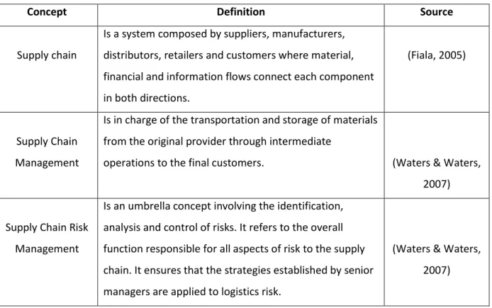
Risk management is the process in charge of managing risks in companies and taking the needed actions that minimize the probability of an unwanted failure (Jüttner, 2005). The objective of supply chain risk management is to capture the potential risk and take right actions to avoid supply chain vulnerability. The importance of supply chain risk management constantly grows in modern times. Table 1 provides the definition of some supply chain concepts.

Concept Definition Source

Supply chain

Is a system composed by suppliers, manufacturers, distributors, retailers and customers where material, financial and information flows connect each component in both directions.

(Fiala, 2005)

Supply Chain Management

Is in charge of the transportation and storage of materials from the original provider through intermediate

operations to the final customers. (Waters & Waters, 2007)

Supply Chain Risk Management

Is an umbrella concept involving the identification, analysis and control of risks. It refers to the overall function responsible for all aspects of risk to the supply chain. It ensures that the strategies established by senior managers are applied to logistics risk.

(Waters & Waters, 2007)

Table1: Concept definitions

Cost pressure forces companies to optimize their supply chain. To increase the efficiency of a producing company, it makes sense to focus on its core competency and outsource other processes, such as transport, storage, distribution (Davis-Sramek et al., 2017). This creates a new dependency on service providers and suppliers and therefore creating risks to the company (Kırılmaz & Erol, 2017). A delay in delivery can lead to a complete paralyze in company production that is why a resilience supply chain risk management is vital for companies to success (Supply Chain Risk Leadership, 2011).

Supply chain disruption is defined as unforeseen events that disrupt the correct flow of goods and materials within a supply chain (Hendricks & Singhal, 2003; Kleindorfer & Saad, 2005; Svensson, 2000) and expose the business to operational and financial risks (Stauffer, 2003).

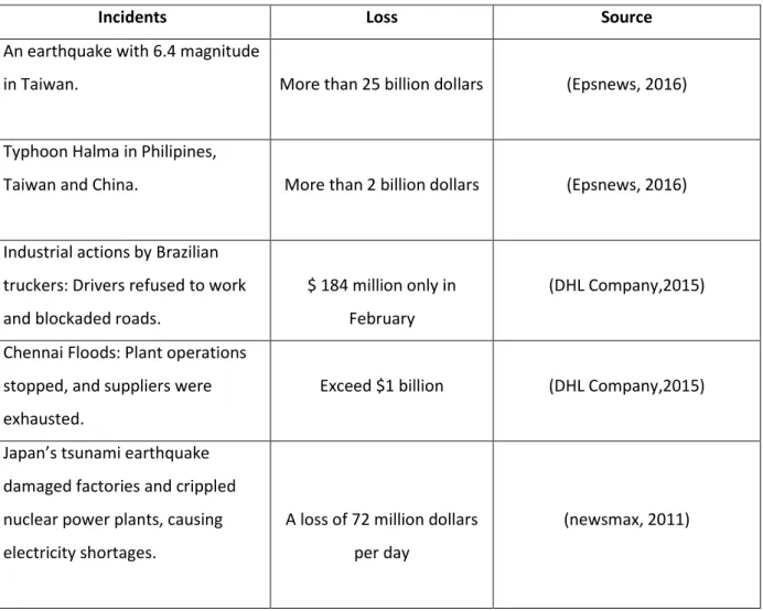
The supply chain council referred in its supply chain operations conference that a single event in a specific location can leads to harmful impact for an enterprise and even cause it to leave an industry (Supply Chain Council, 2012). Several natural disasters or sociopolitical incidents happens in the past

3 led to supply chain disruption and harmful impacts on business and organizations, table 2 lists several events related to supply chain disruption that generated a huge loss within several sectors and organizations for the past recent years.

Incidents Loss Source

An earthquake with 6.4 magnitude

in Taiwan. More than 25 billion dollars (Epsnews, 2016)

Typhoon Halma in Philipines,

Taiwan and China. More than 2 billion dollars (Epsnews, 2016)

Industrial actions by Brazilian truckers: Drivers refused to work and blockaded roads.

$ 184 million only in February

(DHL Company,2015)

Chennai Floods: Plant operations stopped, and suppliers were exhausted.

Exceed $1 billion (DHL Company,2015)

Japan’s tsunami earthquake damaged factories and crippled nuclear power plants, causing electricity shortages.

A loss of 72 million dollars per day

(newsmax, 2011)

Table 2: Incidents caused supply chain disruption

2.2 D

In supply chain industry, a good analytical process can deliver a huge competitive advantage in making the right decisions. Leading supply chain companies are using data analytics to drive their supply chain and extract knowledge to hedge from disruption and optimize their operations (Sanders, 2016). Flight delays are in almost all airports in the world, it occurs in a frequent way especially in busy hub airports. This delay has serious impact on logistics industry and leads to supply chain disruption. Several studies were concentrated on predicting delays using datamining techniques. The challenge is the complexity of the airport processes and the inability of it to analyze data. Some airports are trying to implement solutions, but it is still not intelligent enough to optimize the supply chain. Ariyawansa and Aponso in their paper tried to find out data mining techniques that can be useful to use to improve the airport systems. For the flight delay prediction, they find that the regression analysis, the classification technique of support vector machine, random forest, naïve

4 bayesian classifier and K-nearest neighbors are relevant data mining techniques to be used in such problem (Ariyawansa & Aponso, 2016). Cepeda, Maricruz, Basilio and Jean David has predicted delays in their article delays in supply logistics of offshore platforms. The difference between delivery date and deadline was considered as delays period and converted to categorical variable. They used data mining techniques: first apriori association rules to study possible relations between transactions on the database such as weight versus delay or weight versus type of operations, then used multilayer perceptron neural network to predict cargo delays using voyages features (weekdays, origin, destinations, cargo class) and finally decision tree model to predict delay status and type of operations (Fun-sang Cepeda, A, Basilio, & David, 2015). A method was developed to alarm flight delays based on machine learning method, researchers used as a first step clustering process. They got the delay classes by grouping their data by similarities. As a second step, K means algorithm as well as Bayes model, decision trees, neural network and rule models was used. After that they train their model and compared based on statistical results and find out that decision tree was the performed model (Zonglei, Jiandong, & Guansheng, 2008). In the same topic, Khanmohammadi, Tutun, and Kucuk came up with a model to predict possible flight delays at JFK airport. The study shows that artificial neural network technique is a good approach for such problem, but the challenge was in dealing with nominal variables. As a result of their work, a new type of multilevel input layer artificial neural network was introduced to deal with nominal variables and their model was able to outperform the traditional backpropagation method in terms of the prediction error and time required to train the ANN model (Khanmohammadi, Tutun, & Kucuk, 2016). Karthik Gopalakrishnan and Balakrishnan developed a comparison study of several approaches to predict delays in air traffic networks. They used a developed aggregate model of the delay network dynamics (Markov Jump Linear System), machine learning techniques such as classification and regression trees and three candidate Artificial Neural Network (ANN) architectures. The result of their study was that ANN models are effective for classification problems, however Markov Jump Linear System performed well for regression problems. The study shows that a good delay prediction method depends mainly on the specific type of the problem (classification or regression), the dataset whether it is balanced or unbalanced and the prediction horizon (Gopalakrishnan & Balakrishnan, 2017). Rebollo & Balakrishnan had as objective to predict the departure delay on a particular link or airport. For their study, classification method was used where the target variable is binary of whether the delay is less or greater than a predefined threshold, and regression method where the output is continuous to estimate departure delay along the link. Two years period data was used from the aviation system performance metrics data base. K-means algorithm was used for clustering results on 6 clusters, then random forest approach as an ensemble classifier was used for both classification and regression (Rebollo & Balakrishnan, 2014).

5 To study airport delays and understand its causes, several studies was concentrated on inclement weather and its impact on delays. In their study Allan, Beesley, Evans, & Gaddy was trying to study delay causality at Newark International Airport. They worked on the correlation between different types of weather and its impact on delays. It was concluded that convective weather, thunderstorms and reduced ceiling and visibility are the main factors for large delays at the airport (Allan, Beesley, Evans, & Gaddy, 2001). In the same research topic, Klein, Craun and Lee has developed a predictive model that estimates delays in airports using data from weather forecast. They split the weather component into different types (snow, thunderstorms, wind). They end up with a predictor model that predict timing and magnitude of weather impact on airport delays (Klein, Craun, & Lee, 2010). To implement a predictive model for the arrival delay of a schedule flight, Belcastro, Marozzo, Talia, & Trunfio take into consideration both flight and weather information. Several algorithms (random forest, Stochastic Gradient Descent, Naïve Bayes ,logistic regression) was tested and the random forest algorithm was selected for its performance in terms of accuracy (Belcastro, Marozzo, Talia, & Trunfio, 2016).

3. CONCEPTUAL MODEL

3.1 P

D

S

Currently, our customers are notified about incidents that may impact their supply chain. However, they are not informed about the expected delay caused by a certain incident. Incident and shipment data sources have not been linked. Therefore, the aim of the project is to use historic air freight shipment and historic incident data to understand the effect of incidents on shipment delays. Our company tool provides information on incidents like its category or severity but no information on the exact impact of those incidents on shipments. The final product should be the display of a predicted shipment delay interval within the existing tool, based on historical delays. This project is important for the company customer since they will be able to use historical data shipment milestone to understand typical delays, allows logistics managers to anticipate long delays, readjust production processes, determine required risk mitigation and change shipment modes by alternative sourcing and support cost optimization on inventory. For XXX business units, this project helps to leverage accumulated data to provide a new revenue stream as data provider for supply chain. The emphasis of this project is on risks that threat the supply chain from outside and are beyond the control of the company. This includes several categories such as natural disasters and socio-political incidents. In our project, we are going to focus on shipment delays and try to predict it for a list of airports that our company uses to develop the company product and offer efficient information to our customers. Figure 1 explains better the shipment delays cycle: let’s assume that we have three

6 shipments in airport of Los Angeles, and an incident happens like Cyber-attack leads to airport wide disruptions and then expected delays will happen.

Figure1: Shipment delays cycle

The goal is to improve the customer information management system and provide more accurate and efficient information. Currently, we provide our customer with information that its shipment will be disrupted, the location and the incident categories and description. After the implementation of this project we will provide it with the expected delay interval of his shipment so that he will be able to have an estimated period of the disruption and to take the required initiatives.

3.2 B

P

P

U

A meeting with different company’s business units was set to understand the business need of the project and examine the company shipment processes and procedures. In this meeting, we had a better understanding of the business units and how the shipment process is working to know to which business unit we can request information and data. Shipment delays is defined by the difference between the scheduled and real arrival time of the shipment to its destination. Figure 2 illustrates the company’s shipment route. We are going to predict shipments going from CLS, CFM/DEP to ARR/ARV.

1. Three shipments routed via airport of

Los Angeles 2.Cyberattack leads to airport-wide disruption 3.Terminals revert to manual operations, slowing down productivity and delaying shipments 4.It leads to an interval of X delay time in shipment processing

7 Figure 2: Shipment route

Source: Company’s resource

3.3 D

C

We were looking for historical shipment and incident data with all shipment milestones (i.e., timestamps, origin, destination and intermediate airports, information on expected time of arrival) as well as information on the shipment (size, chargeable weight). We started collecting data from different sources like databases of the group. This step took a very long time as the access to databases within company’s business units require a lot of forms to fill regarding the high security level and the privacy of the needed information. Also, sometimes information needed for the shipment database was manually filled what makes the process more difficult.

3.4 D

C

P

3.4.1 Data

Data cleansing and preprocessing was the most time-consuming and challenging part of the project. Using Excel and SQL Management Studio, we had to analyze both incident and shipment databases and link them together. After establishing the link, we had to link the obtained data with the airport dataset. Also, we had to make some transformations on our existent variables and add eight new variables to the dataset.

3.4.1.1 Incident database

The company tool has recorded incidents from several partners. Data was read and preprocessed, as an example data types were changed, and incident main categories were added to the data. According to our risk management analyst, incidents that are relevant to airports would include either of the two words ‘’airport’’ or ‘’IATA’’ in the incident description. We assumed that major

8 airports operate similarly, therefore we selected the top airports that the company uses for its operations.

3.4.1.1.1 Incident duration

The exploratory data analysis showed problems in the duration of incidents with the ‘’last modified date’’ variable, which we assumed as the end date for calculating the incident duration and the end of an incident. This date was sometimes very recent due to a continuous update, resulting in an unusual long incident duration. The topic was brought to the attention of the team and fixed in collaboration with a partner company, which created a new column ‘’Set to past’’. The company top airports were joined with the incident data via geo-location. For geo-location, latitude and longitude were rounded up and down to the first decimal place.

3.4.1.2 Shipment database

Shipment data was extracted from the shipment database. Then, shipments were converted to UTC time.

3.4.2 Data joining

To join incident dataset with the shipment dataset we created dataset of top airports that the company uses for its operations with their IATA code, ISO country and latitude and longitude. Incident and Shipment data were joined using the following logic: if the shipment was between ‘’incident created’’ and ‘’set-to-past date’’ and at the respective airport where the incident occurred then we join, table 3 represents the variables and its description after the join.

Variable Name Variable Description

Id Incident ID

SHPR_NAME Shipper Name

SHPR_CITY Shipper City

CNSE_ACCT Receiver account

CNSE_NAME Receiver name

CNSE_CITY Receiver city

Ship_delay_binary Shipment duration

num_intermediate_stops Number of stops made per shipment

Categories Incident categories

Destination country Receiver Country

SHPR_ACCT Shipper account number

Severity Severity of the incident

Incident_duration_binary Incident Duration

9

VOL Volume

Airport_Country Shipper country

Table 3: Joiner variables

3.4.3 Variable Transformation

Data preprocessing and transformation have been performed to make data ready for modeling. Due to the lack of variables, we added some variables that we consider it helpful in building the model.

3.4.3.1 Shipment duration

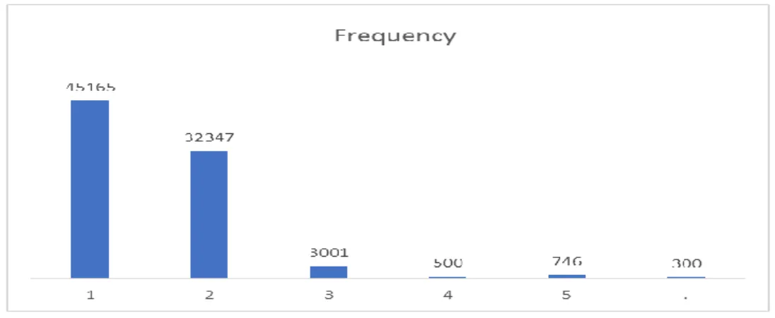
Fig 3 represents the frequency of the shipment delays variable, we split our shipment delays variable into classes using 1day interval. 45165 of the observations have less than one day delay, 32347 have between one and two days of delays, 3001 have between 2 and 3 days, 500 between 3 and 4 days and 1046 more than 4 days. About half of the shipment has less than one day of delays, so we decided to proceed for binary target variable where 0 is shipment duration less than one day and 1 when shipment duration is one day or more.

Figure3: Frequency of shipment delays observations

3.4.3.2 Incident duration

For the incident duration we did the same logic as shipment duration, we convert it to binary variable where 0 is incidents less than one day and 1 are incidents more than one day.

3.4.3.3 Severity

We decided to assign numbers from 1 to 4 for severity variable where 1 is extreme, 2 is severe, 3 is moderate and 4 is minor.

3.4.3.4 Airport Continent

We assigned numbers from one to five for each airport continent: number one was affected to Africa, two to America, three to Asia, four to Australia and five to Europe.

3.4.3.5 Destination Continent

We assigned numbers from one to five to each destination continent: number one was affected to Africa, two to America, three to Asia, four to Australia and five to Europe.

10

3.4.3.6 Other variables

Due to the few numbers of variables available in our dataset, we decided to add variables that we think it will improve our model. For that reason, we added the following variables: destination continent, airport continent, terrorism index airport and destination (Sheffi, 2001), route variable which states the route of the shipment, intercontinental variable in which it take the value of 0 if the shipment is between the same continent and 1 if it is not, international variable which take 0 if the shipment is within the same country and 1 if it is not and average distance variable in which we calculate the average distance between the airport country and the destination country of shipment.

4. MODELING

After preparing the data, the dataset was imported to SAS enterprise miner, a software developed by SAS® Institute Inc. It is required to define the role and level of the remaining variables. Shipment delay variable was identified as our binary target variable.

4.1 D

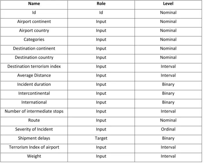
We have 17 variables and 82,059 observations. Table 4 represents the variables imported to SAS software:

Name Role Level

Id Id Nominal

Airport continent Input Nominal

Airport country Input Nominal

Categories Input Nominal

Destination continent Input Nominal

Destination country Input Nominal

Destination terrorism index Input Interval

Average Distance Input Interval

Incident duration Input Binary

Intercontinental Input Binary

International Input Binary

Number of intermediate stops Input Interval

Route Input Nominal

Severity of Incident Input Ordinal

Shipment delays Target Binary

Terrorism Index of airport Input Interval

Weight Input Interval

11

4.2 D

In this part, we will deal with missing values and outliers.

4.2.1 Outliers and missing values

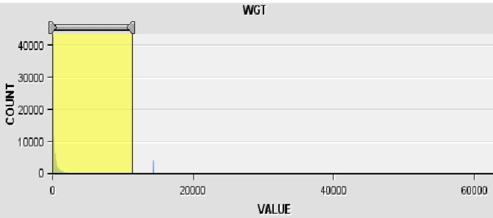
We treated missing values before importing data to SAS enterprise miner, we had missing values within weight variable and we deal with it using average method. By visualization from figure 4, we noticed that there are some observations that can be considered as outliers since they have too high values comparing to most of the observations in the dataset with low frequency.

Fig4: Filter for weight variable

As a result, we will treat as outlier 2648 observations (3.2% from overall observations) that will be excluded from the dataset.

4.3 S

D

When the data is fully preprocessed, the analysis can be started. It is important to validate the model, meaning to check if the model can be used not only to estimate the probability of the depending variable for the observations that we used in the analysis, but also predict the probability for the new one. The model can be constructed using the entire dataset, and then be validated using the same dataset. But then it may result in over-fitting and being too tailored to the given dataset, thus failing to work with new data. Another option is before building the model, we can split the dataset in three parts: training, validation and testing. In this case, training set will be used to build the model, validation set to control the training process and test set to estimate the quality of the model in unseen data. As there are several ways of split it, in our project we chose to use the partition node to split our dataset, where 60% will be used for training, 30% for validation and 10% for testing.

4.4 F

S

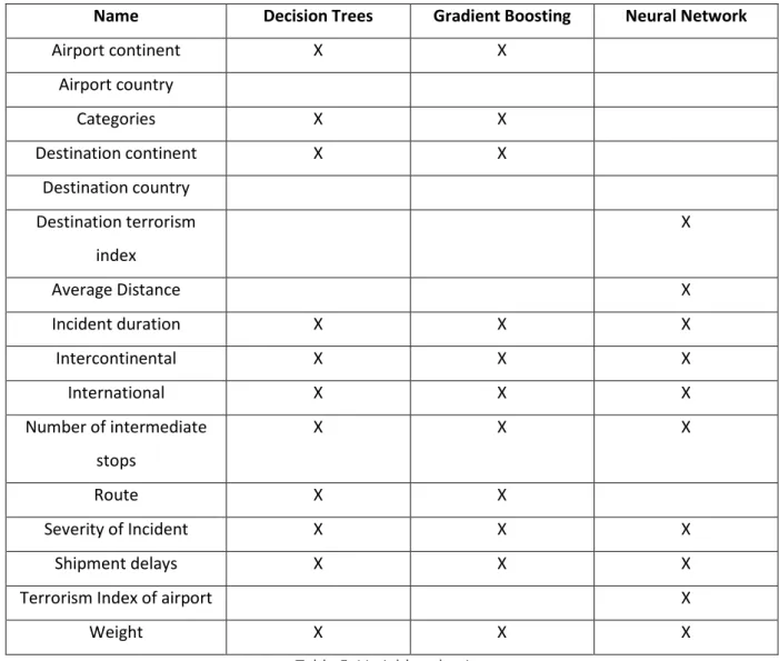
Table 5 presents the variables selected for every algorithm, for neural networks we excluded nominal variables and for the other algorithms we selected all variables.

12

Name Decision Trees Gradient Boosting Neural Network

Airport continent X X Airport country Categories X X Destination continent X X Destination country Destination terrorism index X Average Distance X Incident duration X X X Intercontinental X X X International X X X Number of intermediate stops X X X Route X X Severity of Incident X X X Shipment delays X X X

Terrorism Index of airport X

Weight X X X

Table 5: Variable selection

4.5 B

M

In this part of the project we will build the predictive model.

Data mining is composed by two modeling techniques: Predictive modeling (supervised learning) and the descriptive modeling (unsupervised learning). Supervised learning is where you have input variables and an output variable, and you use an algorithm to learn the mapping function from the input to the output. The goal is to be able to classify new and unknown values given known observations of other variables. When new input data is provided, we can predict the output variables for it. Unsupervised learning is when we only have input data and no corresponding output variables. The aim is to find patterns in the data in order to learn more about the data (D. Hand, 2007). As the main goal of the project is to predict the shipment delays, the task inherent to the study is the predictive modeling. The predictive modeling is divided into two main types of problems: the regression problem and the classification problem which implies to our project. To keep the study simple and easy to understand, the learning algorithms used was chosen based on the results

13 of the previous mentioned studies in the literature review section. Decision trees, multi-layer neural networks and gradient boosting algorithms will be used in this study.

Every learning algorithms has its parameters that should be wisely parametrized. This task consume time and requires knowledge of each algorithm, several combinations was tried manually for each algorithm and the most performed combination was selected (Seminar & Koblar, 2012).

4.5.1 Decision Trees

Decision tree graph represents choices and their results under the form of a tree. The nodes represent an event and the edges the decision rules. A decision tree classifies instances by sorting them from the top (root node) to the down (leaf node). It first selects an attribute to place in the root node making one branch for each possible value (Larose & Larose, 2014). This process is recursively repeated for each branch, using only the instances that reach the branch, where the selection of the best attribute is again made to test at that point of the tree. When all instances of a node have the same classification, it is stopped for that part of the tree. The goal is to have leaf nodes as pure as possible – each leaf only represents records within the same class –with the discrimination between classes (Larose & Larose, 2014). Decision tree can also be represented as sets of if-then rules to simplify the understandability (Rokach & Maimon, 2010). Different algorithms exist for learning decision trees such as CHAID (Chi-square automatic interaction detection) which uses p-value from a significance test to measure the desirability of a split (Milanović & Stamenković, 2016) and Iterative Dichotomiser 3 (ID3) algorithm which uses entropy to calculate the homogeneity of a sample. If it is completely homogeneous the entropy is zero and if the sample is equally divided the entropy is equal to one (Khedr, Idrees, & El Seddawy, 2016). We run our decision trees several times with different parameters (maximum number of branches and maximum number of depth) to obtain the optimal combination. Misclassification method was chosen as an assessment measure to select the best tree. According to SAS enterprise miner, the misclassification method selects the tree that has the smallest misclassification rate.

4.5.2 Multilayer Neural Networks

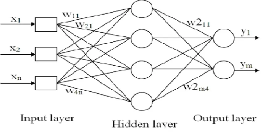
There are different types of artificial neural network, the multilayer perceptron (MLP) is one of them. It is an algorithm inspired from the human brain neural network structure, it is composed by nodes (neurons) where each of them receives input signal (external information) or received by other previous nodes connected via interconnected weights which processes through an activation function to convert the input into output (Ben-David & Shalev-Shwartz, 2014). It is one of the powerful data classification tools, with its ability to learn from the data observation. It is not enough for one single perceptron to learn the amount of information needed to solve complex problems, with the ability to solve only linearly separable problems (Mitchell, 1997). The multi-layer perceptron (MLP) is the solution for this disadvantage and can solve nonlinear problems. There are variety of the

14 neural network structures, the MLP is the most used architecture, it contains a supplementary hidden layer apart from the input and output layers that interconnect them (D. Hand, 2007). One hidden layer is enough to solve most of the complex problems (Palit & Popovic, 2005). In our project, we run our neural network nodes with different number of hidden units to obtain the optimal combination. Misclassification was the selected model criterion which means that the node chooses the model that has the smallest misclassification rate for the validation data set.

Fig 5: Multilayer Perceptron Architecture Source: From (Palit & Popovic, 2005)

4.5.3 Gradient Boosting

Gradient Boosting model is an ensemble of many trees. The trees are not creating in parallel, every tree is depending on the previous tree. The model is based on building different large number of trees and then makes combination of the results from each single tree. The idea is from averaging, the variance could be reduced (Zhang & Haghani, 2015). In our project, we used Gradient Boosting node and set the different parameters needed.

5. EVALUATION

After applying different algorithms, it is time to see which one has the best performance for our problem. Different measurements are available for that

purpose

5.1 C

M

Confusion matrix is a technique allows to see the performance of the classification algorithm. Table 6 represents a 2*2 confusion matrix.

Predicted condition Actual condition Positive Negative

Positive True Positive (TP) False Negative (FN) Negative False Positive (FP) True Negative (TN)

15 The matrix identifies the model’s capability of identifying existing classes in the dataset. Knowing that the negative in our problem is 0 which means the delay is more than one day and positive is 1 when the delay is more than one day, below are the explanation of the confusion matrix:

 True positives (TP): These are cases in which we predicted that the delay is more than one day, and the actual result is the same.

 True negatives (TN): These are cases in which we predicted the delay to be less than one day, and the actual result is the same.

 False positives (FP): These are cases in which we predicted the delay to be more than one day, but the actual result is less than one day.

 False negatives (FN): These are cases in which we predicted the delay to be less than one day, but the actual result is more than one day.

From the confusion matrix, we can derive so many metrics to measure the fitness of a model to a particular context.

5.2 R

/S

It is the proportion of actual positive cases which are correctly identified. It is calculated by the equation below (Kononenko & Kukar, 2007).

Recall= TP/(TP+FN)

Equation 1: Recall Formula

Source: Retrieved from (Kononenko & Kukar, 2007)

5.3 A

(ACC)/C

C

I

(CCI)

It is the proportion of the total number of predictions that were correct. It is the total number of corrected classifications divided by the total number of overall cases as the equation below shows (Kononenko & Kukar, 2007).

CCI=ACC=(TP+TN)/(TN+FP+FN+TN)

Equation2: Accuracy formula

Source: Retrieved from (Kononenko & Kukar, 2007)

5.4 P

It is the total number of true positives divided by the total number of predicted.

Precision=TP/(TP+FP)

Equation3: Precision formula

16

5.5 ROC

C

ROC curve is widely used to measure the performance of supervised classification rules (D. J. Hand & Till, 2001). It refers to the area under the ROC (Receiver Operating Characteristics) curve, the true positive rate (sensitivity, recall) is plotted in function of the false positive rate (100-Specificity) as presented in figure 6. Every point of the curve refers to a sensitivity/specificity pair corresponding to a specific decision threshold. The area under the ROC curve (AUC) represents how well a parameter can distinguish between two groups. The larger is the area the better is the model.

Fig 6: ROC Curve Source: Retrieved from ncss.com

6. RESULTS AND DISCUSSION

The idea was to apply different algorithms and identify the one who will perform better according to our classification problem.

6.1 D

T

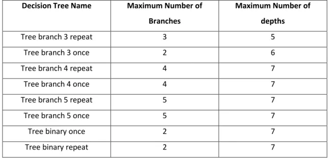
We run our decision trees several times with different parameters searching for the optimal combination. Table 7 presents the different combination used.

Decision Tree Name Maximum Number of Branches

Maximum Number of depths

Tree branch 3 repeat 3 5

Tree branch 3 once 2 6

Tree branch 4 repeat 4 7

Tree branch 4 once 4 7

Tree branch 5 repeat 5 7

Tree branch 5 once 5 7

Tree binary once 2 7

Tree binary repeat 2 7

Table 7: Decision Trees parameters

We used model comparison node to identify the champion model between the several decision trees.

17 Fig 7 represents the cumulative lift chart, since curves are a bit close to each other and we are not going to be able to differentiate among models, we are going to use misclassification rate and ROC curve to decide about the best performed algorithm.

Fig7:Cumulative lift curve for validation

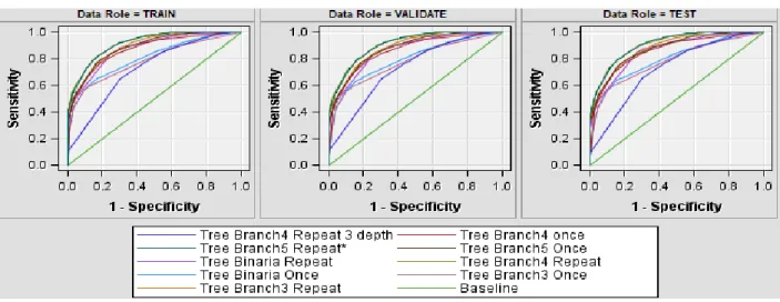
Figure 8 represents ROC curves for each decision tree. From the ROC curves, we can see that decision tree with 5 branches had the largest AUC (Area Under Curve) with ROC index of 0.9, which means that decision tree 5 model has the highest discrimination power.

Fig 8:ROC curve

Before confirming the best performed model, we need to understand our business need and select the measurement that we will base our decision on it. Since our goal is to inform our customer about the delay range, we will select based on the accuracy measurement. Decision tree with 5 branches has the lowest misclassification rate of 0.187 and the highest accuracy rate of 81.3%.

6.2 N

For neural networks, we run the nodes searching for the optimal combination. Misclassification was the selected model criteria. We choose multilayer Perceptron as architecture for all the neural

18 networks and changed the number of hidden units for each neural network. The results of the misclassification rates are presented on table 8 below. Neural network 5 and 4 had the lowest rate.

Neural Network Name Misclassification (Validation)

Neural 5 0.33

Neural 4 0.33

Neural 3 0.34

Neural 2 0.34

Neural 1 0.38

Table 8: Misclassification Rate Neural Networks

According to table 9 which represents the confusion matrix of neural network 5, neural 5 has an accuracy of 70 %, recall of 70% and 68.5% of precision.

False Negative True Negative False Positive True Positive

3414 8597 3683 8014

Table 9: Confusion Matrix Neural5

6.3 G

B

We run our Gradient Boosting nodes. By default, it will build 200 trees, we set for each node different maximum number of branches and depth searching for the optimal combination. We used model comparison node to identify the champion model. Table 10 represents the results of misclassification rate, we can conclude that the trees with 4 branches and 5 branches have the lowest misclassification rate of 23%.

Model Node Name Misclassification rate

Gradient 3 branches 0.24

Gradient 5 branches 0.23

Gradient 4 branches 0.23

Gradient 6 branches 0.24

Gradient 2 branches 0.25

Table 10:Misclassification rate Gradient Boosting

6.4 C

M

After identifying the algorithm that had the best results in every model, we used model comparison node to compare between them and came out with the champion model between neural network with 5 hidden units, decision tree with 5 branches and gradient boosting with 4 branches. Neural

19 networks usually have the best results but due to the limitation in variables decision tree had better results.

6.4.1 ROC Curve

Fig 9 represents the ROC curve, we can see that decision tree had the largest area under curve (AUC) with ROC index of 0.9 while gradient boosting had 0.8 and neural network 0.7, which means that the decision tree model has the highest discrimination power.

Fig 9: ROC Curve

6.4.2 Misclassification

Table 11 represents the misclassification rates for each of the model, decision tree had the lowest misclassification rate of 18%.

Model Misclassification Rate

Decision Tree 0.18

Gradient Boosting 0.24

Neural Network 0.23

Table 11:Model’s Misclassification rate

Decision tree with 5 branches is quite big to interpret, fig 10 represents binary decision tree.

20 We are going to interpret the first three levels of it. The most important variables that play a role for shipment delays prediction are the route of the shipment, the categories of the incidents and its duration. Below are some rules that we can deduct from the decision tree of fig10:

 If the route is one of the following France – United States, United Kingdom - United States, Spain – United State, Ireland - United States, United Kingdom - Turkey, Hong Kong - Mexico, United States – Mexico and the incident duration is more than one day and the incident categories is flight cancellations or weather advisor then it is 98.7% that the shipment delays will be more than one day.

 If the route is one of the following France – United States, United Kingdom - United States, Spain – United State, Ireland - United States, United Kingdom - Turkey, Hong Kong - Mexico, United States – Mexico and the incident duration is less than one day, and the airport continent is in Asia, America or Australia then 92% the shipment delays will exceed one day.

 If the route is one of the following: Singapore – United States, United States - Spain, United States - China, United States - United Kingdom, United States - United States, Israel - Australia, Singapore – Canada and the incident category is travel warning, so it is 100% that the shipment delays will be more than one day.

7. PRACTICAL IMPLICATIONS

This study reinforces the idea that data discovery is needed within corporations for a better understanding of data and then for the business growth of the company. After the implementation of the project, the impact of incident on shipment data is now studied since we can notice that the incident variables are between the most important variables to predict the shipment delays. Managers are now aware about the variables that contribute most to the shipment delays.

The most important variables that play a role for shipment delays prediction are the route of the shipment, the categories of the incidents and the duration of the incident. To avoid shipment delays, managers should find a way to take control of those variables.

The output of this study helps the company to offer information to its customers to allow logistics managers to anticipate maximum delays, readjust production processes, determine required risk mitigation, change shipment modes by alternative sourcing and support cost optimization on inventory. For the company business units, this project helps to leverage accumulated data to provide a new revenue stream as data provider for supply chain.

8. CONCLUSION

The goal of this study was to use historical air freight shipment data and historical incident data to study the impact of incident on shipment delays and identify an interval of the shipment delays to inform customer about it. To achieve our goals, we linked incident data and shipment data to present

21 to the algorithm using Excel and SQL Management Studio. We linked incident database and shipment database using the logic below: if the shipment transaction has occurred within the range of time that the incident happens and at the respective airport then we join. We came out with a shipment-incident dataset which was used to predict the shipment delays. Then, based on the constructed dataset, data preprocessing and the needed transformations was carried out to build a predictive model with the capability to predict the shipment delays using data mining and machine learning techniques. As we saw in the results and discussion chapter, decision tree algorithm performed better, showing that the most important variables that play a role with shipment delays prediction are the route of the shipment, the categories of the incidents and its duration.

9. LIMITATIONS AND RECOMMENDATIONS FOR FUTURE WORKS

Despite the efforts and time made to make the project a reality, some limitations should be acknowledged. The most significant one that restricted the development of the study was due to the few numbers of the variables available, so that we need to include additional variables. In fact, data pre-processing took a significant time and effort conducted in this study. For the future researches it will be better for the company to include additional variables to its databases. Other limitations were the quality of data, further improvement is needed for the way that data is recorded and stored since the shipment transactions were scanned manually which leads to data inconsistency.

22

10. REFERENCES

Allan, S. S., Beesley, J. a, Evans, J. E., & Gaddy, S. G. (2001). Analysis of Delay Causality at Newark International Airport. 4th USA/Europe Air Traffic Management R&D Seminar Santa Fe, New

Mexico, USA December 2001, (July 2000), 1–11.

Ariyawansa, C. M., & Aponso, A. C. (2016). Review on state of art data mining and machine learning techniques for intelligent Airport systems. In Proceedings of 2016 International Conference on

Information Management, ICIM 2016 (pp. 134–138).

https://doi.org/10.1109/INFOMAN.2016.7477547

Belcastro, L., Marozzo, F., Talia, D., & Trunfio, P. (2016). Using Scalable Data Mining for Predicting Flight Delays. ACM Transactions on Intelligent Systems and Technology, 8(1), 1–20.

https://doi.org/10.1145/2888402

Ben-David, S., & Shalev-Shwartz, S. (2014). Understanding Machine Learning: From Theory to

Algorithms. Understanding Machine Learning: From Theory to Algorithms.

https://doi.org/10.1017/CBO9781107298019

Chiang, C., Kocabasoglu‐Hillmer, C., & Suresh, N. (2012). An empirical investigation of the impact of strategic sourcing and flexibility on firm’s supply chain agility. International Journal of

Operations & Production Management, 32(1), 49–78.

https://doi.org/10.1108/01443571211195736

Davis-Sramek, B., Fugate, B. S., Miller, J., Germain, R., Izyumov, A., & Krotov, K. (2017). Understanding the Present by Examining the Past: Imprinting Effects On Supply Chain Outsourcing in a Transition Economy. Journal of Supply Chain Management, 53(1), 65–86. https://doi.org/10.1111/jscm.12131

DHL Company. (n.d.). The Top 10 Supply Chain Disruptions 2015. Retrieved June 10, 2018, from http://www.delivered.dhl.com/en/articles/2015/11/a-look-back-at-2015-the-top-10-supply-chain-disruptions.html

Epsnews. (2016). Top Five Supply Chain Events in 2016. Retrieved June 30, 2018, from https://epsnews.com/2017/02/03/top-five-supply-chain-events-2016/

Fiala, P. (2005). Information sharing in supply chains. Omega, 33(5), 419–423. https://doi.org/10.1016/j.omega.2004.07.006

Fun-sang Cepeda, A, M., Basilio, R., & David, C. J. (2015). Prediction of delays in supply ligistics of offshore platforms (Vol. 217, p. 16). Congreso Internacional Copinaval.

Gopalakrishnan, K., & Balakrishnan, H. (2017). A Comparative Analysis of Models for Predicting Delays in Air Traffic Networks. Twelfth USA/Europe Air Traffic Management Research and

Development Seminar (ATM2017).

Hand, D. (2007). Principles of Data Mining. Drug Safety (Vol. 30). https://doi.org/10.2165/00002018-200730070-00010

Hand, D. J., & Till, R. J. (2001). A Simple Generalisation of the Area Under the ROC Curve for Multiple Class Classification Problems. Machine Learning, 45(2), 171–186.

23 Hendricks, K. B., & Singhal, V. R. (2003). The effect of supply chain glitches on shareholder wealth.

Journal of Operations Management, 21(5), 501–522. https://doi.org/10.1016/j.jom.2003.02.003

Jüttner, U. (2005). Supply chain risk management: Understanding the business requirements from a practitioner perspective. The International Journal of Logistics Management, 16(1), 120–141. https://doi.org/10.1108/13598540410527079

Khanmohammadi, S., Tutun, S., & Kucuk, Y. (2016). A New Multilevel Input Layer Artificial Neural Network for Predicting Flight Delays at JFK Airport. In Procedia Computer Science (Vol. 95, pp. 237–244). https://doi.org/10.1016/j.procs.2016.09.321

Khedr, A. E., Idrees, A. M., & El Seddawy, A. I. (2016). Enhancing Iterative Dichotomiser 3 algorithm for classification decision tree. Wiley Interdisciplinary Reviews: Data Mining and Knowledge

Discovery. https://doi.org/10.1002/widm.1177

Kırılmaz, O., & Erol, S. (2017). A proactive approach to supply chain risk management: Shifting orders among suppliers to mitigate the supply side risks. Journal of Purchasing and Supply

Management, 23(1), 54–65. https://doi.org/10.1016/j.pursup.2016.04.002

Klein, A., Craun, C., & Lee, R. S. (2010). Airport delay prediction using Weather-Impacted Traffic Index (WITI) model. In AIAA/IEEE Digital Avionics Systems Conference - Proceedings.

https://doi.org/10.1109/DASC.2010.5655493

Kleindorfer, P. R., & Saad, G. H. (2005). Managing risks in supply chains. Production and Operations

Management, 14(1), 53–68. https://doi.org/10.1111/j.1937-5956.2005.tb00009.x

Kononenko, I., & Kukar, M. (2007). Machine learning and data mining. Machine Learning and Data

Mining. https://doi.org/10.1533/9780857099440

Larose, D. T. ., & Larose, C. D. . (2014). Discovering Knowledge in Data: An Introduction to Data

Mining: Second Edition. Discovering Knowledge in Data: An Introduction to Data Mining: Second Edition. https://doi.org/10.1002/9781118874059

Milanović, M., & Stamenković, M. (2016). CHAID Decision Tree: Methodological Frame and

Application. Economic Themes, 54(4), 563–586. https://doi.org/10.1515/ethemes-2016-0029 Mitchell, T. (1997). Machine Learning. McGraw-Hill Science/Engineering/Math.

https://doi.org/10.1007/978-3-540-75488-6_2

newsmaw. (n.d.). Toyota Output Loss 40,000 Vehicles. Retrieved March 11, 2011, from

https://www.newsmax.com/finance/headline/toyota-output-loss-japan/2011/03/14/id/389443/

Palit, A. K., & Popovic, D. (2005). Computational Intelligence in Time Series Forecasting.

Automatisierungstechnik. https://doi.org/10.1007/1-84628-184-9

Rebollo, J. J., & Balakrishnan, H. (2014). Characterization and prediction of air traffic delays.

Transportation Research Part C: Emerging Technologies, 44, 231–241.

https://doi.org/10.1016/j.trc.2014.04.007

Rokach, L., & Maimon, O. (2010). Decision Trees. In Data Mining and Knowledge Discovery Handbook (pp. 165–192). https://doi.org/10.1007/0-387-25465-X_9

Sanders, N. R. A. to U. B. D.-S. C. pd. (2016). How to Use Big Data to Drive Your Supply Chain.

24 http://libweb.ben.edu/login?url=http://search.ebscohost.com/login.aspx?direct=true&db=bth &AN=115285409&site=ehost-live

Seminar, I., & Koblar, V. (2012). Optimizing Parameters of Machine Learning Algorithms. Kt.Ijs.Si. Retrieved from

http://kt.ijs.si/marko_debeljak/Lectures/Seminar_MPS/2012_2013/Seminars/Seminar_I_Koblar .pdf

Sheffi, Y. (2001). Supply Chain Management under the Threat of International Terrorism. The

International Journal of Logistics Management, 12(2), 1–11.

https://doi.org/10.1108/09574090110806262

Stauffer, D. (2003). Risk: The Weak Link in Your Supply Chain. Harvard Management Update, 8(3), 3. Retrieved from

http://search.ebscohost.com/login.aspx?direct=true&db=bth&AN=9377221&site=ehost-live Supply Chain Council. (2012). Supply Chain Operations Reference Model - Overview. Supply Chain

Operations Management, 24. https://doi.org/10.1108/09576059710815716

Supply Chain Risk Leadership, C. (2011). Supply Chain Risk Management: A compilation of best practices. Supply Chain Risk Leadership Council, 27–28.

https://doi.org/10.1109/TEM.2009.2013839

Svensson, G. (2000). A conceptual framework for the analysis of vulnerability in supply chains.

International Journal of Physical Distribution & Logistics Management, 30(9), 731–750.

https://doi.org/10.1108/09600030010351444

Waters, C. D. J., & Waters, D. (2007). Supply Chain Risk Management: Vulnerability and Resilience in

Logistics. Kogan Page Limited.

Witten, I. H. , Frank, E., & H. (2011). Practical Machine Learning Tools and Techniques. Machine

Learning. https://doi.org/10.1016/C2009-0-19715-5

Yi, C. Y., Ngai, E. W. T., & Moon, K. (2011). Supply chain flexibility in an uncertain environment: exploratory findings from five case studies. Supply Chain Management: An International

Journal, 16(4), 271–283. https://doi.org/10.1108/13598541111139080

Zhang, Y., & Haghani, A. (2015). A gradient boosting method to improve travel time prediction.

Transportation Research Part C: Emerging Technologies, 58, 308–324.

https://doi.org/10.1016/j.trc.2015.02.019

Zonglei, L., Jiandong, W., & Guansheng, Z. (2008). A new method to alarm large scale of flights delay based on machine learning. In Proceedings - 2008 International Symposium on Knowledge