UNIVERSIDADE NOVA DE LISBOA Faculdade de Ciências e Tecnologia Departamento de Física

(1)

UNIVERSIDADE NOVA DE LISBOA

Faculdade de Ciências e Tecnologia

Departamento de Física

A first analysis of the atmospheric measurements from

TANSO/GOSAT

Bárbara Sofia Santos Teixeira

Dissertação apresentada na Faculdade de Ciências e Tecnologia da Universidade Nova de Lisboa para obtenção do grau em Mestre em Engenharia Física

(a presente dissertação foi preparada no âmbito do Protocolo Sócrates/ERASMUS existente entre a FCT-UNL e a Université Libre de Bruxelles)

Orientador: Prof. Doutor Pierre-François Coheur (ULB)

(2)

2

Agradecimentos

Começo por agradecer ao Professor Pierre-François Coheur, da Université Libre de Bruxelles, por ter coordenado este trabalho mas também pelo seu apoio e conhecimentos transmitidos.

Agradeço também a todas as pessoas pertencentes ao serviço de Chimie quantique et photophysique da Université Libre de Bruxelles.

Aos Professores José Paulo dos Santos e Gregoire Bonfait, da FCT-UNL, pela ajuda prestada durante todo o processo relativo à mobilidade ERASMUS, no âmbito da qual este trabalho foi efectuado.

Aos meus colegas de trabalho na ULB Ariane Razavi, Stéphane Vranckx, Simon Chefdeville, Yasmina R'Honi, Lieven Clarisse e Jean-Lionel Lacour.

Aos meus colegas e amigos da FCT-UNL Daniel Martins e Joaquim Conde, bem como a todos os restantes colegas do MIEF.

À minha família mais próxima, mãe e avó, aos meus amigos e ao Ariën, pelo incondicional apoio ao longo de todo este percurso.

(3)

3

Resumo

Este trabalho analisa os espectros atmosféricos registados pelo instrumento TANSO-FTS a bordo da plataforma GOSAT, com o objectivo de avaliar a utilidade dessas medidas para as aplicações químicas, em especial para monitorizar compostos de azoto reactivo na baixa atmosfera.

Como uma missão dedicada para o clima, GOSAT tem uma série de vantagens sobre outras sondas, como a alta resolução espectral e uma extensa cobertura das regiões espectrais do infravermelho térmico e de ondas curtas de infravermelho. Na primeira parte do nosso trabalho, determinamos, através da realização de um conjunto de cálculos de transferência radiativa, as bandas moleculares que compõem o espectro TANSO-FTS nas diferentes regiões do espectro, e as espécies que poderiam potencialmente ser detectados em condição de alta poluição. Mostramos em particular, que N2O e NH3 têm assinaturas de absorção na banda SWIR número 2, que poderia ser utilizada - a prossecução do trabalho é necessária para uma avaliação definitiva - para melhorar a monitorização da fonte.

Na segunda parte deste trabalho, concentramo-nos nas medições de TANSO-FTS no infravermelho térmico e proporcionar um estudo comparativo com as medidas de radiância validadas e bem estudadas realizada pelo instrumento IASI a bordo da plataforma MetOp. Através de uma inter-comparação sobre os oceanos com rigorosos critérios de co-localização e congruência temporal, mostramos que as radiâncias medidas pelo TANSO-FTS a serem 2 K superiores em relação ao IASI para medições durante o dia, sendo que para a noite, radiâncias do TANSO-FTS a serem 0,7 K inferiores em relação ao IASI. Nós também achamos que a line shape teórica não está perfeitamente adaptada para reproduzir as medições. Essas são questões

que precisam de atenção para uma análise mais sofisticada com GOSAT. Ainda assim, baseando-se num método simples de indexação de radiância e cálculos de diferença de temperatura de brilho, podem comprovar que o TANSO-FTS tem capacidades de detecção considerável de NH3, aparentemente, superiores aos do IASI. O instrumento é indicado para fazer a detecção inequívoca de hotspots numa base diária e permitir capturar as variações sazonais em todos os

(4)

4

Abstract

This work examines the atmospheric spectra recorded by the TANSO-FTS instrument onboard the GOSAT platform, with the aim of assessing the usefulness of these measurements for chemistry applications, and in particular for monitoring reactive nitrogen compounds in the low atmosphere.

As a dedicated mission for climate, GOSAT has a series of advantages over other sounders, such as high spectral resolution and extensive coverage of thermal infrared and shortwave infrared spectral regions. In the first part of our work, we determine, by performing a set of radiative transfer calculations, the molecular bands which compose the TANSO-FTS spectra in the different spectral regions, and the species which could potentially be detected under high pollution condition. We show in particular that N2O and NH3 have absorption signatures in the SWIR band number 2, which could possibly be used – further work is needed for a definitive assessment – to improve on source monitoring.

(5)

5

Index of figures

Fig. 1 – Role sharing in the GOSAT project. (http://www.gosat.nies.go.jp/) ... 14

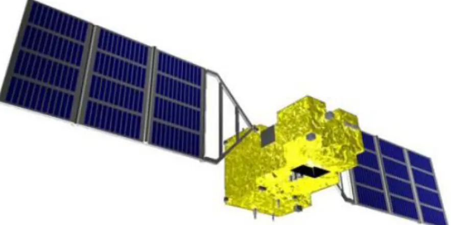
Fig. 2 – Overview of GOSAT in orbit. (http://www.gosat.nies.go.jp/) ... 15

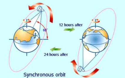
Fig. 3 – Illustration of a sun-synchronous orbit. Figure courtesy of the National Space Agency of Japan (NASDA) ... 16

Fig. 4 – GOSAT observation and orbits. (http://www.gosat.nies.go.jp/) ... 16

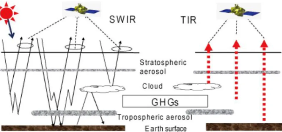
Fig. 5 – Radiance observation by TANSO in the short-wave and visible (left) using reflected/scattered solar radiation and in the thermal infrared (right). (http://www.gosat.nies.go.jp/) ... 17

Fig. 6 – Diagram of a Michelson interferogram. ... 18

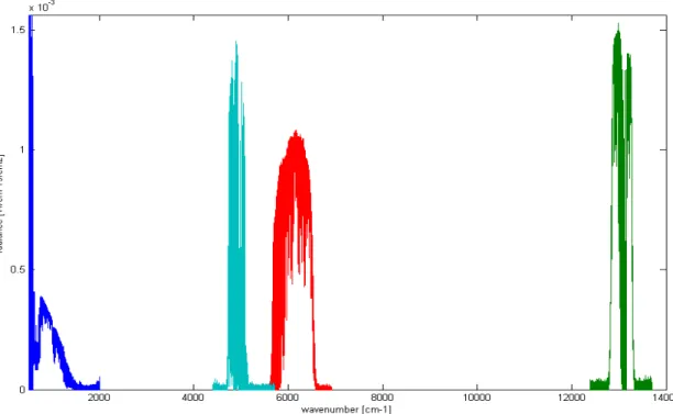
Fig. 7 - Example of a local day-time GOSAT spectrum in the four different spectral bands, from the TIR to the visible. Note: the TIR band was multiplied by a factor or 30 for clarity. ... 20

Fig. 8 – MetOp and IASI (http://www.esa.int/) ... 21

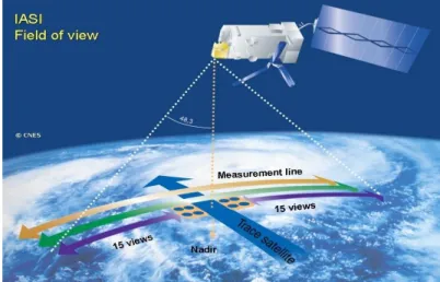
Fig. 9 – IASI observation mode. (http://smsc.cnes.fr/IASI/)... 22

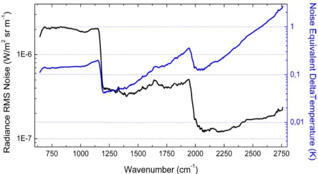
Fig. 10 – IASI radiometric noise over three spectral bands, in radiance units (black curve) and equivalent delta temperature (blue curve) (Clerbaux et al, 2009). ... 24

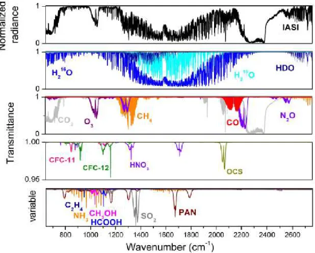
Fig. 11 – Example of an IASI spectrum in normalized radiance (top) and with individual molecular contributions highlighted (three following panels), in descending order of importance. (Clerbaux et al, 2009) ... 25

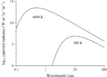
Fig. 12 – Illustration of blackbody curves at 288 K and 6000 K. Note the logarithmic scale of the black-body spectral radiance. ... 27

(8)

8

Fig. 14 –Example of surfaces’ reflectivity. (Petty, 2006) ... 31

Fig. 15 - Specular reflection. (Petty, 2006) ... 32

Fig. 16 - Lambertian reflection. ... 32

Fig. 17 – Individual molecular contributions highlighted for visible band; above Pacific Ocean.37 Fig. 18 – Individual molecular contributions highlighted for SWIR 2 band; above Pacific Ocean. ... 38

Fig. 19 - Unknown signature present in every TANSO-FTS spectrum. ... 38

Fig. 20 – Individual molecular contributions highlighted for SWIR 3 band; above Pacific Ocean. ... 39

Fig. 21 – Individual molecular contributions highlighted for TIR band; above Pacific Ocean. .. 40

Fig. 22 – Night-time spectrum for the thermal infrared range above sea. Left panel: good agreement between TANSO-FTS (blue line) and IASI (red line). Right panel: bad agreement between both satellites. ... 43

Fig. 23 – Left: histogram of brightness temperature differences for IASI and TANSO-FTS spectra occurred during day-time data. Right: same for night-time data (note: no time filter was applied). ... 44

Fig. 24 - Relation between the brightness temperatures measured by both satellites. ... 45

Fig. 25 – Instrumental line shapes for the TANSO-FTS TIR band, provided there is no misalignment in the spectrometer. ... 46

Fig. 26 – Spectral fitting of TANSO-FTS in a narrow portion of the TIR band. ... 47

Fig. 27 – Nitrogen Cascade. (Galloway & Aber, 2003) ... 49

Fig. 28 - Block diagram. ... 50

Fig. 29 - NH3 distribution obtained by TANSO-FTS in 3 days (12th, 13th and 14th of March 2010). ... 52

(9)

9

Fig. 31 - NH3 seasonal variation obtained by IASI: (a) April 2009, (b) July 2009, (c) October 2009, (d) January 2010. ... 54

(10)

10

Index of tables

Table 1 - Characteristics of the TANSO-FTS instrument. ... 18

Table 2 – Characteristics of the TANSO-CAI instrument. (GOSAT, 2009) ... 20

Table 3 – Characteristics of IASI. (Clerbaux et al, 2009) ... 23

Table 4 – Parameters used to simulate the molecules’ profiles. ... 36

Table 5 - List of some molecules absorbing in the TIR band of TANSO-FTS. ... 41

Table 6 – Clear windows used for the cross-calibration. ... 42

Table 7 - Statistical values obtained for both set of data. ... 44

Table 8 - Parameters used to fit the spectrum. ... 47

Table 9 - Vibration modes for NH3; source: HITRAN website. ... 51

(11)

11

Introduction

Earth’s atmosphere has been dealing with several chemical changes during the years which are reflected in the global environment through some phenomena that can destroy the ozone layer or lead to a global warming.

These changes in the global environment can be due to natural factors that have been happening through years such as variations in the solar flux or even changes in Earth’s orbit around Sun since this influence the quantity of energy which is reflected and absorbed (Svensmark & Friis-Christensen, 1997). However, the role played by human in factors that may change global environment has become more important through time. These factors are related with industrial and agricultural activities, in order to give an answer to growing population and an exigent society. They result in the emission of for example greenhouse gases to the atmosphere, or as well of fine particles – the aerosols. There is still another factor that may change the global environment: the land use evolution. Through replacing forest by arable lands or asphalt, Man is modifying the Earth’s surface and its way of reflecting the sunlight and release the heat, which may lead to a temperature rise. Due to all these reasons, it became more important to monitor how atmosphere is changing.

With the advance of the technology to probe the atmosphere from the space (remote sensing) as well as the theoretical models of atmospheric radiative transfer, it has been possible to better understand and know which chemical compounds and processes are responsible for global environmental issues. Combining the global observations to chemistry models makes it possible to identify and quantify the sources of these emissions, allowing not only a better knowledge about this subject but also a step forward in science. There are several space missions with this field of study as their main purpose.

This works reports on a first analysis of the atmospheric measurements made by the TANSO instrument onboard GOSAT satellite, which is a dedicated mission for monitoring climate gases. To support the analysis, the measurements are put in parallel to those of the IASI sounder, which are extensively studied at ULB.

(12)

12

With a global coverage and substantial sampling, this sounder uses the thermal infrared range to probe the composition of the atmosphere. By having a global coverage, it allows to follow the spatial and time evolution of the atmospheric trace gases as well as the aerosols. IASI benefits from a near real-time discrimination of the data (between the moment that the measurements are made by the satellite and the moment they are available to the user, on ground) which enhances scientific return and enables operational application. IASI consists in a Fourier Transform Spectrometer (FTS) associated with an imaging instrument to detect clouds and aerosols.

TANSO (Thermal And Near infrared Sensor for carbon Observation) on board GOSAT (Greenhouse gases Observing SATellite) is also a nadir looking sounder, launched in January 2009 by the Japanese Aerospace Exploration Agency and that is specifically designed to monitor CO2 and CH4 from space during its lifetime of 5 years (Kuze & Suto, 2008). This way, it intends to estimate the greenhouse gases source and sink in a sub-continent scale and verifying if the requirements of the Kyoto Protocol are being achieved. The Kyoto protocol aims to the reduction of the greenhouse gases in the atmosphere during the first period of commitment (2008-2012). As IASI, TANSO is a FTS with high optical throughput and spectral resolution, detecting shortwave infrared (SWIR) and thermal infrared (TIR) spectra. It is coupled to an imaging instrument to detect clouds and aerosols.

This work is thus intended to look deeper in the spectra recorded by TANSO in order to estimate the extent of available in comparison with IASI. In particular, we aim to analyze the possible gain of having higher spectral resolution to monitor trace gases with weak absorptions. Additionally, we intend to examine the measurement in the SWIR and determinate how they can be used for atmospheric chemistry analysis. The species we are more interested in are nitrogen compounds and especially ammonia (Clarisse et al, 2009), for which the first observations from space have recently been made. Specifically, we intend to use the satellites’ measurements of NH3 to try to inform on the nitrogen cycle, study the NH3 seasonal variation above a specific location and what can lead to such variation, and also infer if it is possible to detect patterns of the diurnal cycle.

The importance of monitoring the nitrogen cascade is related with the important implications that it has in our planet. Even though nitrogen is an essential element for life on Earth, along with oxygen, it can be dangerous for living organisms. The inert form (N2) is harmless but the reactive form can be deleterious when it accumulates and cycle in the air, soils or water.

During the last century, the mass production of reactive nitrogen has increased very much due to the needs of society nowadays, which is reflected in the need for food and energy that lead to several environmental issues (Galloway & Aber, 2003), such as:

 Eutrophication and acidification of soils and water

 Air quality

(13)

13

 Malnutrition

The capabilities of satellites to provide global-scale measurements of reactive nitrogen in the environment offers an important opportunity to better quantify nitrogen sources, follow transformation and transport. By using also chemistry models, this would help to better understand the impacts of these reactive species on human and ecosystems health on a regional or global scale.

(14)

14

Chapter 1 TANSO/GOSAT and IASI/MetOp

satellites sounders

1.1 GOSAT science objectives

The Greenhouse gases Observing SATellite (GOSAT, “IBUKI” as it was named by its Japanese creators) was launched on the 23rd of January, 2009 (Yokota, et al., 2009). This project was born from a co-operation between three different Japanese entities each one with their own responsibilities: the Ministry of the Environment (MOE), the National Institute for Environmental Studies (NIES), and the Japan Aerospace Exploration Agency (JAXA). The role sharing is illustrated in figure 1.

(15)

15

GOSAT is the only satellite mission fully dedicated to measuring atmospheric greenhouse gases, and especially CO2 and CH4, for the benefit of climate science and policy. By the time that GOSAT was being developed, in 2003, there wasn’t accurate information of how the greenhouse gases are geographically distributed on the earth and/or how they behave seasonally on the global scale. The decision of launching the first satellite in the world to monitor the greenhouse gases (carbon dioxide, CO2, and methane, CH4) was made with two specific purposes:

 The first scientific objective of GOSAT lies in the need to make accurate estimate of sources and sinks of carbon dioxide (CO2) and methane (CH4) on a sub-continental scale. With this, the aim is to contribute for a better understanding of climate issues by identifying the type and the geographical distribution of those fluxes (i.e., sources and sinks). Using this data, improved knowledge about the global distribution and seasonal variations of the greenhouse gases are expected. In turn, this should improve our understanding and modeling of the global carbon cycle and its influences on the climate.

 The second scientific objective of GOSAT concerns to the expansion of the existing earth observation satellite technology, developing new methods and technologies for greenhouse gases measurements, that should benefit future earth observing satellites.

(16)

16

1.2 GOSAT orbit and TANSO instrument

GOSAT is a sun-synchronous satellite that flies at an altitude of 666 km, approximately. A sun-synchronous satellite has a geocentric orbit that combines altitude and inclination in a way that the satellite ascends or descends over one given point of Earth’s surface at the same local mean solar time.

Fig. 3 – Illustration of a sun-synchronous orbit. Figure courtesy of the National Space Agency of Japan (NASDA)

GOSAT does 14+2/3 revolutions per day and so doing, after a three-day period (44 revolutions in total) it will be back at the same location. The onboard instruments have an external field of view of 15.8 mrad, corresponding to a footprint of 10.5 km approximately (diameter field of view for observation) at the surface, see figure 4.

Fig. 4 – GOSAT observation and orbits. (http://www.gosat.nies.go.jp/)

(17)

17

1.2.1. TANSO-FTS

TANSO-FTS is the central instrument for this work. It observes visible and ShortWave InfraRed (SWIR) radiation of the sun reflected by Earth’s atmosphere and surface as well as the Thermal InfraRed (TIR) radiation from the ground and atmosphere, as shown in the figure 5.

Fig. 5 – Radiance observation by TANSO in the short-wave and visible (left) using reflected/scattered solar radiation and

in the thermal infrared (right). (http://www.gosat.nies.go.jp/)

While the satellite is moving, the FTS observes the same footprint during one interferogram measurement. In special observation mode, the instrument can make multiple observations for the same footprint, thereby improving the signal to noise ratio (SNR). TANSO-FTS does observations over the land on lattice points, which are made at a fixed angle interval in cross-track direction. The FTS detectors cover four bands, one corresponding to visible radiation, two corresponding to shortwave infrared, and one to thermal infrared radiation (see figure 7). Measurements are performed during day and night in the thermal infrared and only during day-time in the SWIR, as these observations require solar radiation. The wide spectral coverage allows detecting numerous molecular bands and infer accurate concentration retrievals.

Note that, there’s a significant difference in the reflected character of sunlight over land and over big water surfaces, like oceans or lakes. Water reflects sunlight specularly in certain directions increasing the radiance signal and hence signal-to-noise. Water bodies are particularly interesting for the shortwave infrared during day-time.

(18)

18

Table 1 - Characteristics of the TANSO-FTS instrument.

Band 1 Band 2 Band 3 Band 4

Band name Visible SWIR SWIR TIR

Spectral range 12900 – 13200 cm

-1 ₅₈₀₀_–_{6400 cm}-1 ₄₈₀₀_–_5200cm-1 ₇₀₀_–_1800cm-1

0.758 – 0.775m 1.56 – 1.72m 1.92 – 2.08m 5.56 – 14.3m

Spectral resolution 0.2cm-1

Target species O2 CO2, CH4 CO2, H2O CO2, CH4

Field of view 15.8mrad (footprint: 10.5km)

TANSO-FTS is an instrument based on the principle of a Michelson interferometer (figure 6); the incoming beam is divided in two beams at 90º that are each reflected by a mirror at the end of the path. In a typical Michelson interferometer, one of the mirrors is moving, so the optical paths are different for the beam. It is such that when they recombine after reflection, positive or negative interference is created. An interferogram is created by changing continuously these path lengths. The inverse Fourier transform of the interferogram, generates the light source spectrum (see hereafter). Through this method, the spectra can be acquired in a wide spectral range with at a high spectral resolution.

Fig. 6 – Diagram of a Michelson interferogram.

The figure 6 shows a diagram of a Michelson interferometer, where M1 is a fixed mirror and M2 is a moving mirror. In the specific case of TANSO-FTS, however, both mirrors are connected by a swinging arm so that they move the same distance but with opposite phases. This way, the scan speed is increased due to a doubled path difference. The interferometer achieves high spectral resolution and the increased speed allows high spatial resolution and sampling without sacrificing any of these characteristics.

(19)

19

the mirror 1, M1, that will be detected and the other part will get through the separator, A1, and be reflected by the mirror 2 (M2). These can be written as:











2



0 2 1 0 1 0

r

k

exp

r

k

exp

r

k

exp



















t

i

t

r

A

t

i

t

r

A

t

i

A

s s



Where A0 the amplitude of the incident beam, rs is the reflectance of the separator, t the transmittance,  the pulse beam, r1 and r2 the distances between the separator and M1 and M2, respectively. This way, the intensity detected by the detector is given by

 





 







k

cos

1

2 2 1









B

I

A

I

Where

 

2 2 2

0

2

~ _A _r _t

B  _s , r₂ r₁2d,k 2~_and ~ the wave number. Thus, the

interferogram is given by

 









 

  



 



 

               ' '' ~ ~ 2 cos ~ ~ ~ ~ ~ 2 cos 1 ~ 0 0 0 I I I d B d B I d B I      



  

The term dependent of the  can be written as the Fourier transform of the spectral distribution. So, by applying the inverse Fourier transform the spectral distribution is obtained:

 



_



  



0 ~ 2 cos ' 2 ~ _ ___ _

 I d

B

In fact a real interferogram is never obtained over an infinite path difference but to a limited maximum, L. The real spectrum is calculated after applying the inverse Fourier transform over the infinite path, convolved by an instrumental function that account for the truncation of the interferogram to a finite path length. The latter has the form of a sinus cardinal function (Hurtmans, 1995):

 

~ 2 '

  

 cos 2~



 2

 

~ sinc



2 ~



(20)

20

Fig. 7 - Example of a local day-time GOSAT spectrum in the four different spectral bands, from the TIR to the visible. Note: the TIR band was multiplied by a factor or 30 for clarity.

1.2.2. TANSO-CAI

TANSO-CAI is a multi-channel imager (Table 2) which is used as supporting instrument to the FTS. It aims at identifying and characterizing clouds or aerosols in the instrument field of view. Depending on these (cloud/aerosol coverage, optical thickness), the FTS data are either discarded if too much affected, or corrected. These corrections are of the utmost importance to provide measurements of CO2 and CH4 at the required accuracy.

Table 2 – Characteristics of the TANSO-CAI instrument. (GOSAT, 2009)

(21)

21

1.3 "Atmospheric Composition and Chemistry-Climate

interactions with GOSAT": Background

–

from IASI and

objectives

The main reason behind the present work is to exploit the measurements of TANSO-FTS in the continuation of the efforts made at ULB to monitor atmospheric composition using infrared satellite sensors, and especially IASI. These objectives have been laid in the proposal “Atmospheric composition and Chemistry – Climate interactions with GOSAT” which was selected as PI contribution in the GOSAT mission project, giving us full unrestricted access to the measurements. Among the specific objectives of the proposal, the comparison of the TANSO-FTS measurements with those of IASI is an essential first step. The IASI instrument is shortly described hereafter.

1.4 IASI/MetOp instrument and mission

The Infrared Atmospheric Sounding Interferometer (IASI) is a nadir looking sounder onboard MetOp (METeorology OPerationnal) meteorological payload. It was launched in 2006. IASI consists in a FTS associated with an imaging instrument, to measure thermal infrared spectra.

IASI was developed in cooperation between CNES (Centre National d’Etudes Spatiales) and Eumetsat (European Organization for the Exploitation of Meteorological Satellites) in order to measure with unprecedented accuracy and sensivity a series of meteorological parameters, and in particular temperature and humidity. Apart of these objectives, IASI aims to measure several trace gases such as O3, CH4 and CO, to make an important contribution for the study of the global atmospheric pollution (Clerbaux et al, 2009).

(22)

22

As TANSO, IASI is a Fourier Transform Spectrometer (FTS) that is associated to an imaging instrument. It measures the emitted TIR spectrum by the system Earth-atmosphere. The carrying MetOp platform has a polar sun-synchronous orbit at an altitude of 817 km with an inclination of 98.7° to the equator. The measurements are taken twice a day, at 9h30 (21h30 in the evening) local time and each orbit takes 101min to be completed. After a whole day, IASI has thus made 14 orbits, similarly to GOSAT.

A major difference between IASI and TANSO lies in the spatial and temporal sampling, with IASI being designed to achieve global coverage at high resolution and sampling to benefit meteorological applications. In order to achieve a global coverage, IASI observes Earth with an angle of 48.3° on both sides of nadir to cover a 2500 km swath across the satellite track. There are a total of 30 fields of views in the swath and each is composed of a matrix of 2x2 pixels. The spatial resolution corresponds to the size of a single pixel, which has a 12km diameter on the ground at nadir. With the global coverage twice daily, IASI provides close to 1.3106 observations per day (in comparison with, approximately, 1104 with GOSAT).

The IASI instrument is equipped with several detectors in order to cover the spectral range that goes from 645 to 2760 cm-1, and this way it is possible to include the strong absorption features from, among others, carbon dioxide (CO2) around 15 µm, ozone (O3) at 9.6 µm, strong water vapor 2 band and the methane (CH4) 3 absorption band.

This broad spectral coverage without gaps is a unique feature of IASI. It is obtained by imaging the radiance onto three different detectors, separating the radiance signal in three bands; the first one between 645 and 1210 cm-1, the second one from 1210 to 2000 cm-1 and the third one from 2000 to 2760 cm-1. The IASI spectral resolution (FWHM) is between 0.35 cm-1 and 0.5 cm-1 for a FTS optical path of 2 cm, depending on the wavelength. For convenience, the standard radiance is apodized by a Gaussian function of 0.5 cm-1 FHWM and this can be considered as the apodized spectral resolution. In table 3 are specified the main features of IASI.

Is also worth to pointing out that the IASI instrument is calibrated in radiance from two common sources: a warm blackbody at 293 K and the cold space at 2.7 K. The IASI expected radiance accuracy is 0.5 K, which was recently confirmed on flight (Illigworth, Remedios, & Parker, 2009).

(23)

23

Table 3 – Characteristics of IASI. (Clerbaux et al, 2009)

Geometry of observation Polar orbit ( 800km); Nadir Special coverage Global and twice a day

Field of view 2x2 pixels corresponding to a footprint of 12km diameter. Pixels/Scanning 120 (30 field of views)

Scanning 48.3º

Spectral range 645 – 2760 cm-1

Spectral sampling 0.25 cm-1_{(8400 channels)}

Spectral resolution 0.5 cm-1

Lifetime 5 years

Data flow per day 1.300.000 spectra

IASI achieves measurements with a fairy low radiometric noise. It can be expressed in terms of either radiances or brightness temperature, which refers to the equivalent temperature of a blackbody radiator. This temperature can be obtained by inverting Planck function (see section 2.1). The noise in brightness temperature (T – noise equivalent delta temperature) connects to the radiance noise L_~

 

T

by,

 

T

e

kT

hc

T

L

T

L

_hc _kT

































_~ _~



₂ _ _~

1

1 ~

For a temperature of 280 K, the radiometric noise of IASI evolves from about

1 2

6 _/

10

2_  _ _ 

m sr m

W for wave numbers between 650 and 1100 cm-1, where the first spectral

band takes place, to ₁_.₅_₁₀7 _/ 2_ _ 1 m sr m

W around 2100 cm-1 (figure 10), both values

corresponding to noise equivalent delta temperatures of about 0.15-0.2 K of an equivalent blackbody at 280 K.

(24)

24

Fig. 10 – IASI radiometric noise over three spectral bands, in radiance units (black curve) and equivalent delta

temperature (blue curve) (Clerbaux et al, 2009).

(25)

25

Fig. 11 – Example of an IASI spectrum in normalized radiance (top) and with individual molecular contributions

(26)

26

Chapter 2 Atmospheric radiative transfer

(non-scattering atmosphere) applied

to GOSAT

The remote sensing of the atmosphere is usually made by optical techniques and divided in two different groups: active and passive.

To better understand the work that was made and the analysis of the spectra obtained by TANSO and IASI satellites, this section discusses the physical principals inherent in the analysis of passive sounding in the infrared domain.

2.1 General formulation

1

When an isothermal cavity is under thermodynamic equilibrium conditions, the radiation within this cavity is in equilibrium with the cavity walls and therefore, the spectral energy density depends only on frequency and temperature. If there’s a small hole in the cavity, the emitted radiation will have the same form as radiation within the cavity and is called blackbody radiation.

Planck’s function for a blackbody is given by the following equation:

 

   



 _



1 ²

³ 2

T k hv v

B

e c

hv T

B

Where B_{represents the spectral density in}W/m2 Hz, h_{is the Planck constant,}_the

frequency, cthe speed of light, kBthe Boltzmann constant and T the blackbody’s temperature. At the temperatures of 288K and 6000K, Earth and sun that are the major source of radiation for the

1_{Reference (Andrews, 2000).}

(27)

27

atmosphere, can be considered as blackbodies. The maximum of the radiation emitted by Earth belongs to the thermal infrared range while the radiation emitted by the sun covers the ultraviolet to the infrared, peaking in the visible (figure 12).

Fig. 12 – Illustration of blackbody curves at 288 K and 6000 K. Note the logarithmic scale of the black-body spectral

radiance.

In nature a pure blackbody is rarely encountered but most real bodies can be fairly well described by a grey-body. The spectral emittance, e, represents the fraction of spectral radiance

emitted by a grey body in relation to a blackbody and therefore, e ≤ 1. According with

Kirchhoff’s Law for a given temperature and frequency, e=αwhere α represents the fraction of

energy per unit of frequency interval falling on a body that is absorbed.

The quantity that describe the radiation collected by a remote sensing optical sounder is the spectral radiance, L_v

 

r,s . It describes the flux of photons emerging from or arriving on a small area A with unit normal s, centered at a point r as shown in the figure 13 and it is

measured in _ 2 1 1 Hz sr m

W .

Fig. 13 – Illustration of the solid angle definition.

(28)

28

radianceL_v will decrease in ds. According with Lambert’s law, the fractional decrease of the

spectral radiance is proportional to the density of absorbing or scattering material encountered by the beam along the distance ds

     

s s L s ds dL_v 



_e



_a _v .

With



e being the extinction coefficient (



e 



a 



s where



a is the absorption

coefficient and



_sis the scattering coefficient) and



_a being the density of the active gas. But the gas itself can also emit photons at the frequency v_{and in that case an additional term should be}

added to the previous equation. We have therefore obtained the Radiative-transfer equation:



v v



a e

v _L _J

ds dL

 

  

Which is general form of the radiative transfer equation. In equation (2.3) J_v

 

s is called the source function.

For the sake of simplicity we will consider here only a non-scattering atmosphere, meaning free of clouds and aerosols. In that case, the scattering coefficient is



s 0 and the

extinction coefficient is



e 



a. This way, the attenuation of the radiation through a thin layer of

the atmosphere can be written as

ds I dIabs 



a 

While the radiation emitted by that same layer is given by

ds B ds

B

dIem 



e  



a 

Where B is the Planck function for a blackbody at a given temperature (equation (2.1)). So, in a non-scattering atmosphere, the net change of intensity is:



B

I



(29)

29

This equation is the Schwartzschild’s equation and is generic for all descriptions of absorption/emission processes in the atmosphere. Analyzing this equation makes it easily to infer if there is emission or absorption of radiation through a particular line of sight. That is, when

0

 I

B means that the radiation emitted by the thin layer is greater than the attenuation of the

radiation in that same layer, and thus, there is emission of radiation through the layer. On the contrary, when BI 0 the effect of attenuation is greater than the emission and therefore, there is a decrease of radiance through the layer.

Considering the optical depth, , defined as the negative logarithm of the fraction of radiation that is removed from a beam by scattered or absorbed on a path, as a vertical coordinate since it corresponds to the vertical path from Earth's surface to outer space, we can manipulate the Schwartzschild’s equation to become,

B I d

dI _ _

 With   d ds ds dI d

dI _ _

,



B I



ds dI

a 

 and

a d ds   1 

 . If we multiply each side of the equation

(2.8) by e-, we have:





      



      















Be

d

e

dI

Be

I

e

d

dI

e

B

I

e

d

dI

e

Integrating along the optical depth, we have:





   

_



     

















' 0 ' 0 ' 0 ' 0 ' 0

'

0 '

'

          



d

Be

e

I

d

Be

e

I

d

Be

d

e

dI

This equation is another fully generic form of the atmospheric radiative transfer in a non-scattering atmosphere. It tells us that the radiance has two different components. The first one

(2.8)

(2.9)

(2.10)

(2.11)

(30)

30

represents the attenuated contribution of any radiation source in the far side of the path. For the case of a satellite in orbit looking at the surface, the term I(’) is the intensity of Earth’s surface while the term e- is the transmittance from the whole atmosphere along the considered path. The second term of this equation (the integral) represents the integration of the thermal emission in each point along the line of sight, attenuated by the transmittance between the sensor and ’.

2.2 Simplification for the TIR

2

For the thermal infrared range it is possible to make a simplification, in the formulation of the radiative transfer considering that only the thermal emission/absorption are occurring (no reflection from the sun on the surface).

Therefore, in the case of a nadir looking satellite, like TANSO or/and IASI, that receives thermal infrared radiation from the Earth/atmosphere, and assuming that thermodynamic equilibrium prevails (meaning that the source function can be expressed by Planck’s function

v v B

J  ), the solution of the radiative transfer equation can be written as:

 





 



   

  

 





 Τ , 0,

0 v s v v v

v dz B T

z z z T B L

Where T(z) is the atmosphere’s temperature, Ts is the surface’s temperature and v

 

0, is the

spectral transmittance between the z and the satellite. If there is no extinction along the path (in a non-scattering atmosphere) then the satellite only sees surface emission:

 

s v v B T L 

That is, the radiative transfer equation is given by Planck function for a temperature Ts that it is the surface temperature. This way, it is possible to infer what the surface temperature is by inverting Planck function. More generally, radiance measured by the satellite can be converted into an equivalent temperature called brightness temperature, which would vary with the extinction signatures in the atmosphere.

 

        v B L c hv k hv v T ² ³ 2 1 ln

2_{Reference (Andrews, 2000)}

(2.13)

(2.14)

(31)

31

2.3 Formulation for the SWIR; reflectivity of surfaces

As seen before, GOSAT takes measurements not only in the thermal infrared range but also in the shortwave range. The incident radiation is no more dominated by the Earth thermal radiation which rapidly drops to vanishing values below 4 m (see figure 12) but by reflected solar radiation onto surfaces.

Fig. 14 – Example of surfaces’ reflectivity. (Petty, 2006)

The figure 14, shows that the reflectivity of natural surfaces are strongly dependent of wavelength. Here we make the assumption that the reflectivity is independent of whether the sun shines, from East/West or North/South, which means that is azimuthally isotropic (referred to the horizon), and the dependence upon the zenith angle (referred to the vertical direction, 0°) can be ommited.

So, based on these assumptions it is possible to relate the monochromatic flux, which is

the power per unit area per unit wavelength





                  , lim 0 F

F , with the incident flux by

the simple equation.

0 , ,  

 r F

F _r 

Where  is the zenith angle,  the azimutal angle and ris the surface’s reflectivity, which is only

dependent of the wavelength. The reflectivity integrated over the shortwave is known as the albedo rSW:

SW

SW a

r 1

(2.16)

(32)

32 Where aSW is the absorptivity in the shortwave range.

When the radiation that comes from the sun strikes natural surfaces, it can be reflected in several ways. What is usually done in modeling the radiative transfer is to simplify the formulation considering two different ways of reflection: specular or Lambertian.

In the case of a specular reflection, the flux incident is reflected with the same angle as it was incident on surface.

Fig. 15 - Specular reflection. (Petty, 2006)

For the second case of a Lambertian surface (schematized in the following figure), the reflection is equal in all directions.

Fig. 16 - Lambertian reflection.

And then we have,

 

_{ }

 

 









         



















2 0 2 0 2 0 2 0 0 0

cos

,

cos

,

d

I

d

sen

I

F

a

I

F

r

I

Where d is the solid angle. When the intensity is isentropic, that is when it is constant in all directions, we get to:

  _ _

I

F 

When solving the radiative transfer equation in the SWIR the incident flux term I

 

' of

(33)

33

(34)

34

Chapter 3 Objective of this research

This work is intended to provide a first analysis of the TANSO-FTS measurements in the thermal infrared and the short-wave infrared. The aim is to qualitatively evaluate the information that can be extracted regarding trace gases that are important for atmospheric chemistry, and that could complement measurements made by IASI thermal infrared sounder and others.

This objective is thus not in using GOSAT for its principal purpose (greenhouse gas monitoring) but more in trying to extract from it additional products of reference to the community of atmospheric researchers. The focus is given to reactive nitrogen compounds and in particular ammonia, for which there is a high interest in global remote sensing considering the lack of data.

(35)

35

Chapter 4 Results and discussions

In this Chapter are presented the results obtained in this work, as well as the inherent conclusions. First, are shown the results obtained for the short-wave infrared, followed by the thermal infrared results, radiometric cross-calibration between TANSO-FTS and IASI, spectral calibrations and instrument response function, and finally, the results regarding the monitoring of reactive nitrogen compounds.

4.1 TANSO measurements in the SWIR

4.1.1. Overview per band

In this section, the main goal is to identify the molecular signatures in a TANSO-FTS spectrum in the shortwave infrared range. For that, we used the radiative transfer program called Atmosphit that provides the user with an atmospheric ray tracing, a sophisticated formulation of atmospheric radiation and an optionally a fitting tool. Atmosphit solves the radiative transfer equation (2.12) line-by-line, using spectroscopic parameters from up-to-date databases and atmospheric profiles of pressure, temperature and gaseous concentration. The source function is modeled by a gray body in the thermal infrared. For modeling the short-wave infrared, an effective reflectivity is used for the reflected solar radiation.

(36)

36

This file can be divided in three different parts: geometry (used to simulate the spectrum), spectrometer and molecular multiplicative model to fit. In the first group (geometry) is defined the limits of the atmosphere, the geometry type (ground or nadir) and some parameters about the light source (temperature and efficiency). For the second group (spectrometer) is present the information about the observed spectrum, that is: spectral limits and calibration factor parameters, the signal to noise ratio (SNR), the spectrum type (radiance or transmittance), the maximal optical path difference (MOPD) value of the interferometer, the apodization function and the field of view parameters and finally, the baseline parameters. Lastly, in the third group we find the information about the molecules and multiplicative factors to be simulated and fitted.

Table 4 summarizes the reference parameters used for the TANSO-FTS spectral simulations.

Table 4 –Parameters used to simulate the molecules’ profiles.

Apodization Internal FOV Calibration

Spectrometer

ILS type MOPD (cm) Aperture

4.58496×10-5

Boxcar 3.01

(FWHM = 0.2 cm-1₎ 0.4530°

Baseline Spectrum type

Source temperature (K)

Blackbody efficiency

Ground reflectivity

Transmittance 320.67 0.9627 -

Geometry Limits of the atmosphere (km) Line of sight Earth Radius

0.0 666 Nadir + radiosity 6371.230

This way, for each spectral range – visible and shortwave infrared – the method used can be described in the following steps:

1. Change the concentration of each molecule, in the FIN file, that we want to simulate to produce detectable – but at the same time sometimes unrealistic – absorption signatures, as well as the other parameters that might be changed

2. Load the input files: spectrum, BMD file, FIN file and HITRAN file 3. Compute the spectrum line-by-line by solving the radiative transfer

4. Divide the blackbody function to the simulated spectrum to produce equivalent transmittances (normalized radiances)

5. Plot the obtained results for each molecule

After these five steps, we obtain the normalized transmittance for each molecule individually. We identify those species which contribute to the extinction of radiation and one (potentially for some) threshold by TANSO-FTS.

(37)

37

signatures of H2O and week absorption of CO2, there is also seen a strong signature of O2 which is the molecule that TANSO-FTS aims to measure in this spectral band (see table 1).

Fig. 17 – Individual molecular contributions highlighted for visible band; above Pacific Ocean.

For the second band, identified as SWIR 2, the target species are carbon dioxide and methane (see table 1). Those species strongly contribute to the TANSO-FTS spectrum. We could identify three more absorbing species in this spectral range: water, hydrochloric acid (HCl) and acetylene (C2H2), as shown in figure 18. For C2H2 and HCl the signatures only appear by largely increasing the species concentrations in our simulation. This means that they would only be detectable in particular conditions, above large emission sources (e.g. fires, volcanoes) (Clerbaux

et al, 2009). More work is needed to check if these species would indeed be measurable by

(38)

38

Fig. 18 – Individual molecular contributions highlighted for SWIR 2 band; above Pacific Ocean.

Interestingly, there is a feature in the SWIR spectrum that wasn’t identifiable to the species listed in HITRAN, as shown in figure 19 centered around 6285 cm-1. We are still looking for more information that can lead us to identify this molecular absorption shows up in every TANSO-FTS spectrum.

Fig. 19 - Unknown signature present in every TANSO-FTS spectrum.

V

ar

ia

bl

(39)

39

For the second band of the shortwave infrared range, SWIR 3, the GOSAT target species are water vapor and carbon dioxide, which have indeed strong absorption (figure 20). In addition, that spectral band also includes contribution from CH4, N2O and to lesser extent O3. Finally, although weak, there is a possible contribution of NH3 to that part of the spectrum.

Fig. 20 – Individual molecular contributions highlighted for SWIR 3 band; above Pacific Ocean.

4.2 TANSO measurements in the TIR

4.2.1. Overview

Similarly to what is done above, here we present results from a set of forward simulations in the thermal infrared, to better characterize GOSAT measurements and provide a first basis of comparison to IASI. The spectra that is used for this purpose is the same as above, and was recorded above Pacific Ocean during the month of March 2010.

Like it was done for the shortwave infrared and visible bands, we used Atmosphit line-by-line radiative transfer model to compute the spectra, following the same methodology, to

V

ar

ia

bl

(40)

40

highlight the principal absorption signatures in the spectra. All the parameters that were used are present in table 4.

The next figure shows the molecules that contribute to the spectrum in the thermal infrared range. It is similar to figure 11 (shown for IASI) but is specific to the TANSO-FTS instrument.

Fig. 21 – Individual molecular contributions highlighted for TIR band; above Pacific Ocean.

Within this range of wave numbers, the target molecules for GOSAT are the strong absorbers carbon dioxide (CO2) and methane (CH4). But as we know from IASI experience, there are a number of species that can be detected in high pollution areas or specific fire or volcanic plumes. (Clerbaux, 2009; Clarisse, Clerbaux, Dentener, Hurtmans, & Coheur, 2009). The identifiable species are grouped according to their absorbing strength in table 5.

V

ar

ia

bl

e

V

ar

ia

bl

e

V

ar

ia

bl

e

V

ar

ia

bl

(41)

41

Table 5 - List of some molecules absorbing in the TIR band of TANSO-FTS.

CO2 CH4 O3 N2O HNO3 SO2 NH3 CH3OH

C2H2

C2H4

C2H6

OCS

Strong

absorber ● ● ● ●

Medium

absorber ●

Weak

absorber ● ● ● ● ●

Besides the molecules that are listed in table 5, we also demonstrate the possible contribution of hydrogen cyanide (HCN), hypochlorus acid (HOCl), hydrogen peroxide (H2O2) and nitrogen dioxide (NO2) even though all these molecules have very small features in the spectrum with variable transmittances. They are unlikely to be observed because of very strong interferences with the main absorbers (H2O, CO2, CH4).

4.2.2. Radiometric cross-calibration between TANSO-FTS and IASI

The absolute radiometric accuracy of sounders as IASI or GOSAT is of the utmost importance because the atmospheric radiative transfer in the thermal infrared comes in propagating the Earth’s source function through the atmosphere. A bias in the radiometric calibration induces errors on the entire radiative transfer, which translates in important errors on the retrieval of trace gas abundances. IASI was shown by cross-calibration with the AATSR instrument to meet its target absolute accuracy of 0.5 K (Illigworth, Remedios, & Parker, 2009). Here we provide a comparison between IASI and TANSO-FTS radiances, which is essential for future use of the TANSO infrared radiances for chemistry applications.

For a more accurate comparison in terms of radiance, it’s better to consider surfaces with constant emissivity, good temporal and spatial agreement, observed with similar fields of view because radiances from thermal infrared range of the TOA vary strongly with the wavelength, temperature and emissivity of the surface, atmospheric temperature, atmospheric composition (especially humidity) and with clouds. Due to these reasons, the ideal surfaces are the oceans because their surfaces have a constant emissivity and small temporal variations in temperature. This way, it’s not advisable to use land surfaces since the temperature vary very rapidly and the radiance has a strong dependence of the angle of vision.

In order to do a cross-calibration, the brightness temperature measurements should indeed be done for a same geographical location (latitude and longitude wise) and for a similar time.

(42)

42

1. Selection of reference area above the Pacific Ocean: 20ºlat 5º and

º 115 º

135  

 lon

2. Selection of 10 “clear windows” in each TANSO-FTS and IASI spectrum. We consider a clear window a spectral range where there’s no absorption of any molecule for those wave numbers. They are reported on table 6.

3. Filter in latitude and longitude: only the spectra which have a difference in latitude and longitude less than 0.2º are analyzed

4. Time filter: only the IASI and TANSO-FTS spectra with a time difference less than 3 hours were analyzed

5. Calculate the Brightness Temperature (BT) for these spectra and compute the difference _BTIASI __BTTANSO-FTS_.

6. Filter in cloud coverage: only the IASI spectra with cloud coverage less than 15% were analyzed. IASI cloud information is provided operationally through the Eumetsat dissemination system. Cloud information from GOSAT were not available and hence, all TANSO-FTS data have been kept in the first phase of the analysis.

Table 6 – Clear windows used for the cross-calibration.

Wave number (cm-1)

IASI channels

GOSAT channels

786.25 – 790.75 566 – 580 712 – 734

822 – 823.5 709 – 715 892 – 899

829.5 – 834.5 739 – 759 929 – 954

866.5 – 869.75 887 – 900 1115 – 1131

898.5 – 904.25 1015 – 1038 1276 – 1305

1102 – 1105.3 1829 – 1842 2300 – 2316

1123 – 1133 1913 – 1953 2405 – 2456

1139 – 1147.5 1977 – 2011 2486 – 2528

(43)

43

Fig. 22 – Night-time spectrum for the thermal infrared range above sea. Left panel: good agreement between TANSO-FTS

(blue line) and IASI (red line). Right panel: bad agreement between both satellites.

Figure 22 shows a GOSAT and IASI spectrum collocated in space and time (see section 4.2.2) for the thermal infrared range, recorded during night-time. In the left panel, the spectra coincide well. A noticeable difference lies in the strength of the absorption lines, which is a direct consequence of the different spectral resolution. The higher resolution TANSO-FTS spectrum shows lines with larger strength. In the right panel, the spectra do not coincide that well in terms of their radiance values, likely pointing to remaining clouds in the dataset.

(44)

44

Fig. 23 – Left: histogram of brightness temperature differences for IASI and TANSO-FTS spectra occurred during

day-time data. Right: same for night-day-time data (note: no day-time filter was applied).

Table 7 summarizes the results for the statistics made for both histograms data. Obviously the large standard deviation in both cases points to the presence of clouds or aerosol-containing scenes in on or another dataset, which leads to BT values up to 15K.

Table 7 - Statistical values obtained for both set of data.

IASI & GOSAT day-time IASI & GOSAT night-time

Mean (K) 2.07716 -0.7009

Standard deviation (K) 7.2762 5.23924

Median (K) 2.2689 -0.1637

Based on the information from the histograms and statistics, we can say that there is a significant bias of GOSAT day-time spectra when compared with IASI spectra, for the same conditions (location, cloud coverage and time). The 2K bias can have large impact on the retrieval of trace gases and will have to be addressed urgently if the TANSO-FTS data are to be used for chemistry applications.

(45)

45

Fig. 24 - Relation between the brightness temperatures measured by both satellites.

(46)

46

4.2.3. Spectral calibrations and Instrument response function

In the same way that radiometric calibration is important, the spectral calibration and knowledge of the instrument response function is crucial in retrieving trace gases abundances from high-resolution measurements.

The instrument line shape function (ILS) depends on the theoretical spectral resolution (in a case of a FTS it depends on the optical path difference) and on the optical alignment of the interferometer. In the case there is no post apodization applied, the instrumental line shape of a FTS is a sinc function (Kuze & Suto, 2008).

Fig. 25 – Instrumental line shapes for the TANSO-FTS TIR band, provided there is no misalignment in the spectrometer.

(47)

47

Table 8 - Parameters used to fit the spectrum.

Apodization Internal FOV Calibration

Spectrometer

ILS type MOPD (cm) Aperture

4.58496×10-5

Boxcar 3.01

(FWHM = 0.2 cm-1₎ 0.4530°

Baseline Spectrum type

Source temperature (K)

Blackbody efficiency

Ground reflectivity

Transmittance 320.67 0.9627 2×10-2

Geometry Limits of the atmosphere (km) Line of sight Earth radius

0.0 666 Nadir + radiosity 6371.230

As can be seen from figure 26, although the sinc function reproduces fairly well the lines, there remain residual features larger than the noise around the strongest absorptions. This suggests some distortion of the instrumental line shape. Currently, we have no information on the TANSO-FTS line-shape besides the theoretical sinc function. As for the radiometric calibration this would need to be addressed before more geophysical studies are carried out.

(48)

48

4.3 On the potential use of TANSO/GOSAT for monitoring

the nitrogen cycle

4.3.1. The perturbed cycle of reactive nitrogen

3

In this section will briefly introduce the importance of reactive nitrogen cycle for the atmosphere and how complex it can be, as well as some ways to improve its impacts.

It is known that the total amount of nitrogen (N) in the atmosphere, soils and water is approximately 4×1021g (4×1015 tons!), but most of it (99%) is not available for the majority (99%) of the organisms. The reason for this is that the nitrogen is present in the form of N2 and this form cannot be assimilated by living organisms.

The nitrogen compounds can be divided in two groups: the non reactive, where N2 is the only form of it, and the reactive forms, including all the biologically, photochemically and radiatively active N compounds in Earth’s atmosphere and biosphere, that is accumulating in the environment, in all spatial scales, drastically since 1960 due to the largest increase in human production, compared with other systems. This accumulation can be due to different reasons:

1. Generalization of the cultivation of vegetables, rice and others, allowing the conversion of the non reactive form of nitrogen (N2) into organic nitrogen through biological nitrogen fixation (BNF)

2. Burning of fossil fuels that converts N2 and fossil N into nitrogen oxide (NOx)

3. The Haber-Bosch process that is used to sustain food production and industrial activities. In this process the N2 is converted into a reactive form of ammonia (NH3): N2 (g) + 3 H2 (g) 2 NH3 (g), with the latter used in ammonia-based fertilizers.

It is expected that the production of Nr keep increasing due to the increased population and the accumulation of Nr can contribute to:

 Serious respiratory illness, cancer and heart diseases induced by the production of tropospheric ozone (O3) and aerosols

 Biodiversity reduction in some natural habitats

 Acidification that can also lead to biodiversity reduction in lakes in regions of the globe.

 Eutrophication (increased of chemical nutrients concentration in an ecosystem so that increases the primary productivity of the ecosystem), hypoxia (dissolved oxygen becomes reduced in concentration to a point detrimental to aquatic organisms living in the system) and loss of biodiversity and degradation in costal ecosystems.

 Global climate change and stratospheric ozone depletion, having serious impacts on human and ecosystems health.

(49)

49

Fig. 27 – Nitrogen Cascade. (Galloway & Aber, 2003)

The cycle of reactive nitrogen is based on the multiple connections among the atmosphere and terrestrial and aquatic ecosystems. There are a multitude of impacts in each of these systems but because of the rapid cycling, once it starts, the source of Nr is now irrelevant and the consequences can be up to global. This is the nitrogen cascade introduced by (Galloway & Aber, 2003).

The atmosphere receives Nr coming from air emissions of NOx and NH3, N2O – that has a residence time in the atmosphere of 100 years and it has been increasing at a rate of 0.25%/year – from land/aquatic ecosystems and of NOx from burning fossil fuels. Short lived species such as NOx and NHx (NH3 and NH4+) can accumulate in the troposphere on a regional scale, which some local effects were described above, but with global impacts that are also important to mention. One of these is the importance that NH3 has by rapidly forming aerosols on the radiation balance and global climate, with likely a dominating cooling effect.

4.3.2. Measuring NH

3

from GOSAT: method

UNIVERSIDADE NOVA DE LISBOA Faculdade de Ciências e Tecnologia Departamento de Física