ABSTRACT: The detection, location, identiication and recognition are very important activities for the air forces. Imaging systems are tools used for those functions, so it is mandatory to characterize those systems to really know their actual operational limits. This paper presents a set of measurements for spectral, radiometric and spatial camera characterization to be applied to imaging systems operating in the thermal infrared. A SC5600 camera manufactured by FLIR® Systems was used and assembled with lenses of 27 or 54 mm equivalent focal length. The camera spectral characterization was done by comparison to a calibrated system composed by thermal source, monochromator and a broadband reference detector. The radiometric characterization was performed using an extensive blackbody (CI Systems) for temperatures between 10 and 55 °C to evaluate the camera accuracy and obtain the calibration curves. The spatial characterization was carried out using the same extensive blackbody and 2 standard USAF 1951 machined targets, one made of steel and other of aluminum, serving as masks for the blackbody. Using recycled material, a homemade extended blackbody for outdoor use was built. The results obtained using the 2 blackbodies in laboratory were similar.
KEYWORDS: Infrared, Camera, Calibration, USAF 1951, Blackbody.
Operational Measurements for Infrared
Camera Characterization
Geraldo Mulato de Lima Filho1, Robert Cardoso Fernandes de Almeida1, Ruy Morgado de Castro2,
Alvaro José Damião2
INTRODUCTION
An imaging system is generally composed by a collector (usually lenses and/or mirrors), ilters, detector, processor, a system for data storage and an output unit. he output can be a monitor that provides an image of the collected electromagnetic radiation. he operational wavelength range of the imaging systems is usually between 0.35 and 15 µm (Lillesand and Kiefer 1994). In addition, every electro-optical system has its unique characteristics and some internal parameters to be settled, which directly implies on the quality of the images to be acquired. his quality may or may not be suitable for target location, identiication and/or recognition (Johnson 1958), under certain environmental conditions (atmospheric, altitude etc.) or the scenario in which the target was encompassed (Pace and Sutherland 2001). his paper presents results for a camera with spectral response between 2.5 and 5.1 µm. he measurement procedure can be applied to cameras having diferent spectral responses, if the respective sources and masks for characterization are available.
he complete characterization of these imaging systems is necessary for knowing the operational limits of the equipment. For example, in the case of using a thermal camera for operational purposes, as search and rescue or maritime patrol, one must previously know: what is the electromagnetic spectrum range at which the camera operates and what is its relative sensitivity (spectral characterization)? What is the accuracy on the electromagnetic radiation measurement (radiometric characterization)? What is the actual field of view of each detector element, or how detailed is the target at a certain distance/altitude (spatial characterization)?
1.Departamento de Ciência e Tecnologia Aeroespacial – Instituto Tecnológico de Aeronáutica – Programa de Pós-Graduação em Aplicações Operacionais – São José dos Campos/SP – Brazil. 2.Departamento de Ciência e Tecnologia Aeroespacial – Instituto de Estudos Avançados – Divisão de Fotônica e Geointeligência – São José dos Campos/SP – Brazil.
Author for correspondence: Alvaro José Damião | Departamento de Ciência e Tecnologia Aeroespacial – Instituto de Estudos Avançados – Divisão de Fotônica e
Geointeligência | Trevo Coronel Aviador José Alberto Albano do Amarante, 1 – Putim | CEP: 12.228-001 – São José dos Campos/SP – Brazil.
Once this characterization methodology was applied to a thermal camera, the performance characteristics would be known and this would allow choosing the best camera settings as well as planning the search l ight to maximize the mission success.
h ere are other characteristics to check in an electro-optical sensor (Bower et al. 2009), such as: temporal resolution — the range the sensor revisits, more applicable to satellite sensors; noise equivalent power (NEP) — the minimum amount of radiant l ux to be received by the sensor, to be equal to the noise of the sensor; noise equivalent irradiance (NEI) — the minimum irradiance to be perceived by the sensor, to be equal to its noise; and the noise equivalent temperature dif erence (NETD) — the smallest temperature dif erence that can be measured by the camera. However, at the operational level, the knowledge of the spectral resolution, radiometric resolution and spatial resolution is primary to mission success.
MATERIALS AND METHODS
h e characterization of a thermal or visible camera com-prises 3 steps: spectral, radiometric and spatial. h e camera evaluated in this study was a SC5600 by FLIR® Systems. It is a
high-performance thermal imaging camera for industrial and educational use. It has an array of 640 × 512 pixels, with frequency between 5 and 100 Hz. h e detectors are chilled indium antimonide (InSb), with spectral response between 2.5 and 5.1 µm (FLIR® Systems 2017). h e SC5600 camera used
in this study had 2 optical assemblies, one with an equivalent focus of 27 mm and the other, of 54 mm, both by FLIR® Systems.
h e optical assemblies had an integrated autofocus system. According to the data sheet, the SC5600 has high sensiti-vity, precision and speed, keeping an excellent linearity. h e smallest observed temperature difference is described as 20 mK (0.020 °C). h e SC5600 camera can perform temperature measurements from 5 to 300 °C, and the integration time can be adjusted by increments of µs.
SPECTRAL RESPONSE
An indirect method was chosen to determine the spectral response. It uses a broadband calibrated detector as reference (Schumaker 1996). h e schematic diagram of the experimental arrangement is shown in Fig. 1a and basically includes the following equipment:
• Acton SpectraPro 2500i monochromator — Acton Research Corporation 2003.
• Wide Band Detector Judson Mercury Cadmium Telluride — Judson Technologies LLC 2002.
• Stanford Lock-in Amplii er SR510 — Stanford Research Systems 2013.
• Illuminator IR 6363 Newport® — Newport Corporation
2012.
• Power Supply Newport® 69931 — Oriel Instruments
2002.
• Filters of Edmund Optics® — Edmund Optics 2009.
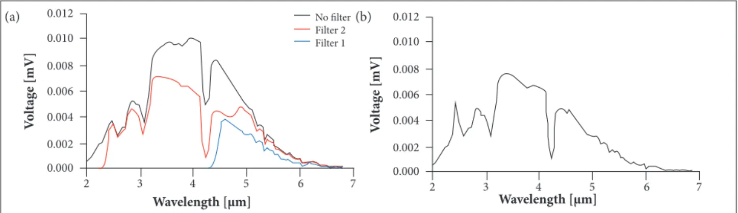
h e results obtained by the Judson detector were used as standard for the camera. Figure 1a shows the schematic diagram and Fig. 1b, the camera assembled for measurements, where: 1 is the camera; 2 is the Judson detector (not assembled); 3 is the monochromator; and 4 is the data acquisition computer. h e Judson detector is at the center of Fig. 1b, but it was not assembled for measurement at that moment. Three sets of measurements were registered for the Judson detector and also for the camera: no i lter, i lter 1 (long pass 4.5 µm) and i lter 2 (long pass 2.5 µm).
h e determination of the spectral response was done in a roundabout way. It used a source, monochromator and a cali-brated detector. h e camera response was compared to the detector one. h e measurements were made in the same ambient as well as geometric and lighting conditions (Zolin Neto 2012).
Figure 1. (a) Schematic diagram of the experimental arrangement; (b) Camera assembled for measurements.
Oscilloscope Lock-in
Microcomputer Monochromator Amplifier Detector
Filter
Chopper
Illuminator Power
4 2
3
1 (a)
RADIOMETRIC CHARACTERIZATION
The experimental arrangement (Fig. 2) was used to perform the radiometric characterization, where 1 represents the camera and 2, the blackbody. In this arrangement, in addition to the camera, it is also used a blackbody SR800 (CI Systems 2004). The camera was placed perpendicularly to the blackbody surface, at 1.55 m. This distance was chosen so the complete Schott’s Contrast Transfer Function (CTF) could be obtained for the spatial characterization. For all measurements, the largest thermalization time was awaited. According to the camera manufacturer, this time is 2 h. An integration time of 1.6 ms was chosen, as recommended by FLIR® Systems, for temperatures between 10 and 55 °C. The
sample rate was 60 Hz. For each established temperature in the blackbody, the data provided by the camera were the medium value of digital levels. For radiance and target temperature measurements, the surface emissivity was considered equal to 1 for the blackbody and 0.97 (aluminum) for the target.
was also painted black, because, even ater sandblasting, it showed some specular relection.
1
2
121.1
10.8 mm
292.8
303.
5 27.
2
292.
8
46.7 47
181.5
303.5
187.7
0 8 . 0
0 8 . 0 0 8 . 0
0 3 . 5 ( × 4 )
Came r a SC5600
B l ackbody an d T arget USAF 1951
Figure 2. Experimental setup for radiometric characterization.
SPATIAL CHARACTERIZATION
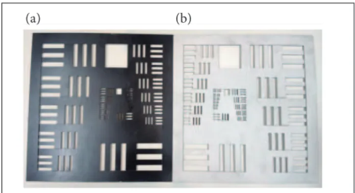
For spatial characterization, 2 standard-based targets USAF 1951 (Applied Image Inc 2017) were machined. he target drawing, dimensioned in mm, is presented in Fig. 3. hey were used as a mask for the blackbody (Fig. 4). he 2 targets/masks, one in aluminum and the other in steel, were produced by the Divisão de Suporte Tecnológico of the Instituto de Estudos Avançados (Fig. 5). he plates were square-shaped with 303.5 mm sides to be embedded in the extensive blackbody SR800 CI Systems, as a mask. he targets were sandblasted to increase the surface roughness, thereby reducing the specular reflection and increasing the Lambertian behavior of the electromagnetic waves relected on the surface. he steel target
Figure 3. Mask fabrication drawing (dimensions in mm).
Figure 5. Steel (a) and aluminum (b) blackbody masks.
Figure 4. Spatial characterization arrangement with aluminum mask in front of the blackbody.
The blackbody was switched on, its temperature, adjusted to 40 °C, and the 1951 USAF metallic target was kept at room temperature (23.6 °C for steel and 22.4 °C for aluminum, measured by thermocouple). The absolute temperature difference between the blackbody and the target was enough to take the spatial characterization data, having the required radiometric contrast.
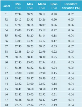
he data collection time was 1 s to guarantee there were no signiicant parameter changes along acquisition. hen, 60 samples of every image were obtained. he medium value of 60 values of each line (black or white) was obtained. A virtual mask was stablished to get the data and as many pixels as possible were evaluated for each pair of line pairs. For the highest spatial frequency, only 4 pixels were evaluated, as there was no room for more pixels. his virtual mask allowed the direct comparison between diferent temperature sets. Figure 6 presents the labels for data collection (Table 1) concerning the aluminum mask at room temperature and the blackbody at 40 °C.
For the target requirement fulill the image, the target-to-camera distance of 1.55 m was chosen for the 27 mm focal length lens. Half and twice of this distance were also measured. he emissivity for the target used was 0.97. his is the value for the aluminum plate, as it has bigger area than the blackbody (emissivity equal to 1) on the image.
Data were analyzed and processed by Altair software (FLIR® Systems 2012). he medium values of the white lines
(warmer, the blackbody) and the dark ones (colder, USAF 1951
target) were obtained. hese values allowed to calculate the relative contrast, which is given by Eq. 1, normalized by the highest value.
Label Min (°C)
Max (°C)
Mean (°C)
Span (°C)
Standard deviation (°C)
31 37.94 38.22 38.12 0.28 0.07
32 23.12 23.33 23.26 0.20 0.05
33 37.90 38.16 38.09 0.26 0.06
34 23.08 23.30 23.19 0.22 0.06
35 38.02 38.20 38.14 0.18 0.04
36 23.03 23.21 23.12 0.17 0.04
37 37.90 38.23 38.15 0.33 0.07
38 22.88 23.10 22.99 0.22 0.05
39 38.16 38.41 38.30 0.25 0.05
40 22.83 23.03 22.94 0.21 0.05
41 38.28 38.52 38.43 0.24 0.05
42 22.80 23.00 22.90 0.15 0.04
43 38.42 38.57 38.50 0.21 0.04
44 22.82 23.00 22.92 0.18 0.04
45 38.41 38.60 38.50 0.19 0.04
46 22.82 23.03 22.92 0.21 0.04
47 38.36 38.55 38.47 0.19 0.04
48 22.65 22.84 22.75 0.19 0.04
Table 1. Data acquired from labels in Figure 6.
Figure 6. Data collect for the aluminum mask at room temperature and the blackbody at 40 °C.
57.27 54.86 52.32 49.63 46.75 43.67 40.34 36.73 32.75 28.31 23.28
oC
A
B
where: A is the average value in digital levels of the emitted radiation (through the bar area) by the blackbody; B is the average value in digital levels of the emitted radiation by the bar area from the Air Force Target 1951 (Fig. 7).
(1)
Figure 7. Area where the data were collected for each line pairs.
A – B
A
+
B
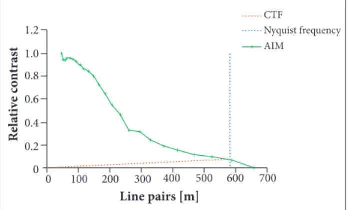
Having those values, the calculations of the CTF (Schott 2007) were held. Figure 8 shows the theoretical CTF preconized by Schott (2007), where the y-axis is the relative contrast described above.
the lowest amount of modulation detected by a system (i.e., other threshold). It is called Aerial Image Modulation (AIM) and it is the minimum required modulation to produce a response by the system (Almeida 2007). Any point below this curve must be disregarded (Fig. 8).
HOMEMADE BLACKBODY
In order to give more mobility to the experiments, a homemade blackbody was built, using spare parts of other systems. he main parts were:
• Digital Temperature Gauge and Controller, Robertshaw, LFS model, with K-type thermocouple (Chromel-Alumel), with measuring range of 70 –1,200 °C (Fig. 9, item 1);
• A 3-L plastic tank (Fig. 9; item 2);
• A water pump, responsible for liquid circulation (Fig. 9; item 3);
• Serpentine (radiator) in a closed circuit with a fan for cooling;
• Resistance nickel-chromium (15 – 25% Cr, 19 – 80% Ni, with the remainder Fe) to heat the liquid; • A copper sheet of 30.3 × 30.3 cm (painted with black
ink on the front) with a copper coil welded on the back part;
• hermal insulator at the back of the blackbody (Fig. 9; item 4); and
• hermocouple (Fig. 9; item 5).
0 1 2 3 4 5 6 7 8 9 10
1.0
0.8
0.6
0.4
0.2
0.0
Line pairs [m]
R
el
at
ive
c
o
n
st
ra
st CTF
AIM Nyquist frequency
Resolution limit
Figure 8. CTF, AIM and the resolution limit (Schott 2007).
NYQUIST FREQUENCY CALCULATION
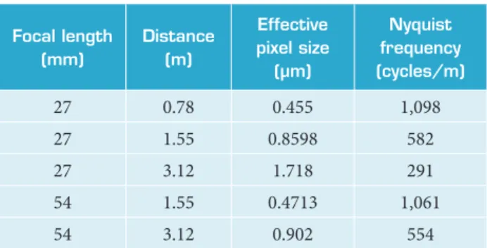
he camera threshold resolution is limited by the Nyquist frequency, which is the inverse of 2 times the efective pixel size, and this (representation of the image) can be calculated using the total number of pixels of the target image and the actual size of the target. If the optical assembly is changed, a new value of the Nyquist frequency must be evaluated. he pixel size was calculated using the total number of pixels (353) in a row, corresponding to a line in the image target of 303.5 mm real size, for a distance of 1.55 mm from the camera. he value of the efective pixel size was 0.8598 µm, and the correspondent Nyquist frequency was 582 cycles/m. his calculation was extended to the other distances and focal lengths (Table 2). Due to rounding on the igures of the efective pixel size, the values of the Nyquist frequency presented some diferences. he line that connects the intersection of the CTF/Nyquist frequency curves to the graph origin indicates
Focal length (mm)
Distance (m)
Effective pixel size
(µm)
Nyquist frequency (cycles/m)
27 0.78 0.455 1,098
27 1.55 0.8598 582
27 3.12 1.718 291
54 1.55 0.4713 1,061
54 3.12 0.902 554
Table 2. Nyquist frequency calculated for the 2 focal lengths and distances evaluated.
Figure 9. Main parts of the homemade blackbody.
1
2 3
5 4
(a) (b)
RESULTS AND DISCUSSION
SPECTRAL CHARACTERIZATION
taken as reference for camera data. Voltage measurements were performed for wavelengths from 2 to 7 µm at intervals of 50 nm. Three data sets were measured: no filter, filter number 2 and filter number 1 (Fig. 10a). The monochromator harmonics were subtracted, and the resulted plot is presented in Fig. 10b.
The camera replaced the Judson detector, and the same set of data was taken in digital levels to get the camera response curve —data obtained with shutter closed, no
Figure 10. (a) Wide Band Detector Judson Mercury Cadmium Telluride; (b) Monochromator harmonics subtracted.
D
ig
i
ta
l l
ev
el
Dig
ita
l l
ev
el
14,000
12,000
10,000
4,000 6,000 8,000
2,000 0
2 3 4 5 6
Closed No filter Filter 1
7
Wavelength [µm]
14,000
12,000
10,000
8,000
6,000
4,000
2,000
0
1.0 2.0 3.0 4.0 5.0 6.0
Wavelength [µm]
N
o
rma
liz
ed
r
es
p
o
ns
e
sp
ec
tr
a
l o
f the SC5
6
0
0
N
o
rma
liz
ed r
es
p
o
ns
e [%]
1.0
0.8
0.6
0.4
0.2
0
2 3 4 5 6 7
Wavelength [µm]
100
20 30 40 50 60 70 80 90
10 0
1.0 2.0 3.0 4.0 5.0 6.0
Wavelength [µm]
V
o
l
tage [mV
]
0.012
0.010
0.008
0.006
0.004
0.002
0.000
2 3 4 5 6
No filter Filter 2 Filter 1
7
Wavelength [µm]
V
o
ltage [mV
]
0.012
0.010
0.008
0.006
0.004
0.002
0.000
2 3 4 5 6 7
Wavelength [µm]
Figure 11. (a) Camera spectral characterization; (b) Monochromator harmonics subtracted.
filter and filter number 1 (Fig. 11a). The monochromator harmonics were subtracted, and the resulted plot is presented in Fig. 11b. The units were those available on the Altair Software.
The response curves provided by the manufacturer and the one obtained in this study can be compared (Fig. 12). The manufacturer’s calibration process and data are not available, so the general curve behavior could be considered satisfactory.
Figure 12. Response curves obtained is this study (a) and provided by the manufacturer (b).
(a) (a) (a)
RADIOMETRIC CHARACTERIZATION
For a set of blackbody temperatures, the temperature measured by the camera was registered (Fig. 13). Diferences from +0.25 to −1.5 °C were found between the surface temperature set in the blackbody and the temperature measured by the SC5600 camera, using an emissivity of 0.97. hese diferences could be raised by factors that were not investigated as the value for the emissivity used may not be the real one, and the relected radiation from surroundings may not have been considered correctly.
Another comparison was made between the calculated radiance and the one provided by the camera. The calcu- lated radiance was obtained from the radiance emitted by the blackbody at the respective temperatures and the radiance reflected on it, coming from the laboratory (Fig. 14). A negligible difference was found. The calculated value of radiance does not include the radiance emitted by the environment air layer. Probably this was one of the factors that caused the difference between the calculated and measured radiances.
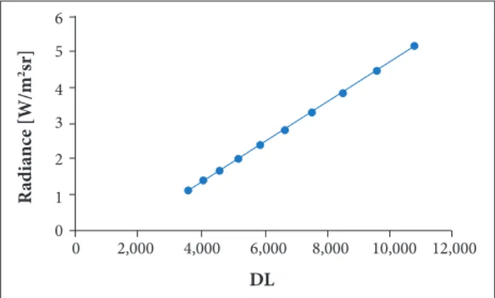
The information provided by the camera is in digital levels. he conversion of the digital levels (DL) to radiance (L) is presented in Fig. 15. he linear dependence is clear. It also allows, for example, that a calibration curve for temperature be obtained.
0.5
0
–0.5
–1.0
10 20 30 40 50 60
Blackbody temperature [°C]
–1.5
–2
∆
T
[
oC]
R
adi
a
nc
e [W
/m
2sr
]
6
5
4
3
2
1
0
0 2,000 4,000 6,000 8,000 10,000 12,000
DL
6
5
4
3
2
1
0
0 10 20 30 40 50 60
Calculated Measured
Temperature [oC]
R
adi
a
nc
e [W/m
2sr
]
Ny quist frequ en cy CTF
AIM
700 600 500 400
Line pairs [m]
R
el
at
ive
c
o
n
tr
ast
300 200 100 0 0 0.2 0.4 0.6 0.8 1.0 1.2
+
+
+ +
+ + +
+ + + + + + + + + + + +++ + +
+ Figure 13. Temperature difference between what was set in
the blackbody and measured by the camera.
Figure 14. Calculated radiance and that provided by the camera.
Figure 15. Conversion from DL to L.
SPATIAL CHARACTERIZATION
The camera was assembled with a 27-mm lens; an integration time of 1,600 us was set, and no filters were used; the steel target was at 23.6 °C (temperature measured by thermocouple) and the blackbody, at 40 °C. The distance between camera and blackbody was 1.55 m. It can be noted in the steel target that the 23rd and 24th elements on the 1951
USAF stayed below the sensor’s resolution limit (Nyquist frequency); the 22nd element has been cut by the lack of
contrast (AIM; Fig. 16). The 21st element was the last solved
within the system’s resolution limitation and with enough contrast. Each line of this element contains about 1.07 mm in width as the distance from the camera to the target was 1.55 m; each pixel in the sensor array provides 0.040° of
ef f ective field of view. The results are summarized on Table 3, where n.a. means “not available”.
For a 12 °C temperature diference, the 2 sets of lenses were tested at diferent distances. he idea was to evaluate the behavior of the CTF curves, having enough contrast condition, guaranteed by temperature diference. he distance taken for the previous data was 1.55 m for the 27-mm lens. Now it was evaluated the data for distances of 0.78 and 3.12 m (Fig. 19). As expected, the number of line pairs resolved was diferent. For the 54-mm lens, distances of 0.78 and 3.10 m were evaluated. Due to space limitations in the laboratory, the distance of 6.20 m could not be assessed.
Table 4 shows the resolution obtained for each available distance. It must be noticed that 2 effective instantaneous ields of view (EIFOVs) could not be determined (Table 3), as the smallest line of pairs was resolved far under the Nyquist frequency.
Focal length (mm)
Distance (m)
Line pairs (cycles/m)
EIFOV (°)
27 0.78 1,098 n.a.
27 1.55 582 0.040
27 3.12 291 0.035
54 1.55 1,061 n.a.
54 3.12 554 0.017
Table 3. Effective ield of view for 2 sets of lenses and different camera blackbody distances.
Figure 17. (a) CTF (aluminum mask, room temperature; blackbody, 40 °C); (b) Last line pairs resolved.
Nyquist frequency
CTF
AIM
700 600 500 400
Line pairs [m]
R
el
at
ive
c
o
n
tr
ast
300 200 100 0 0 0.2 0.4 0.6 0.8 1.0 1.2
+
+ + + + + + + + + + + + + + + + + + + + + +
+
Line pairs [m]
R
el
at
ive
c
o
n
tr
ast
Nyquist frequency CTF
AIM 1.2
1.0
0.8 0.6
0.4
0.2 0
0 100 200 300 400 500 600 700
Figure 18. CTF results for very small temperature difference (0.12 °C) — blackbody at 22 °C.
EVALUATING THE UNCERTAINTY
Small conductance problems were found when using the steel target. Due to the target machining process, there was no physical contact between the ends of each tribar. he target was then replaced by one made of aluminum, whose conductivity showed best results (more uniformity).
he blackbody temperature was set between 10 and 55 °C, in steps of 5 °C, and all the CTFs showed similar proiles. he 23rd and 24th elements were below the sensor’s resolution limit
(the Nyquist frequency), and the 22nd one was disregarded due
to lack of contrast, being below the uncertainty bar touching the AIM curve. he 21st element was the last solved within
the system’s resolution limitation and with enough contrast (Fig. 17). Each line of this element contains about 1.07 mm in width and, as the distance from the camera to the target was 1.55 m, each pixel in the sensor array provided a target efective ield of view of 0.040°.
Smaller temperature differences between target and blackbody were analyzed. he smaller the diference, the worse the spatial resolution obtained. As an example, the aluminum target was set at 22.06 °C and the blackbody, at 21.90 °C. he temperature diference was of 0.16 °C, and the obtained result still presented a proile similar to that proposed by Schott (2007). Figure 18 shows that the 22nd – 20th elements
were cut in the target due to lack of contrast (AIM); the 19th
element could be also disregarded because the uncertainty bar is in the AIM curve, indicating to be in the contrast limit. he 18th element was the last solved within the system’s
resolution limitation and with suicient contrast. Each line of this element contains approximately 1.5 mm wide as the distance from the camera to the target was 1.55 m; each pixel in the sensor array provided efective ield of view of 0.055°.
(a)
Nyquist frequency CTF
AIM
700 600 500 400
Line pairs [m]
R
el
at
ive
c
o
n
tr
ast
300 200 100 0 0
0.2 0.4 0.6 0.8 1.0 1.2
+ +
+++++++ +++
+ +
+ +
+ + +
+ +
+ + +
+
Nyquist frequency CTF
AIM
700 600 500 400
Line pairs [m]
R
el
at
ive
c
o
n
tr
ast
300 200 100 0 0
0.2 0.4 0.6 0.8 1.0 1.2
+
+ + + + + + + + + + + + + + + + + + + + + +
+
OUTDOOR EXPERIMENT
T he homemade blackbody non-uniformity was compared to the one of CI Systems. The blackbodies were set at the same temperature (with a measurable uncertainty) to compare results. The emissivity was set to 0.97 instead of 1, but this does not impede the comparison. The average temperature over the whole square (drawn over the blackbody surface and indicated by numbers 1 and 3 in Fig. 20) was compared. The standard deviation was the same, but the homemade one showed smaller span (Table 3).
In order to perform the experiment in non-controlled conditions, such as in laboratory, it was performed an outdoor experiment. The camera was assembled with a 27-mm lens, and the distance was 1.55 m. The CTF was obtained with the aluminum target at 28.14 °C and the blackbody, at 45.46 °C, both measured by the camera (Fig. 21). It presented a profile similar to that proposed by Schott (2007). It was observed that the 23rd and 24th target
elements were below the 1951 USAF sensor’s resolution limit (the Nyquist frequency). The 22nd element was the
last solved within the system’s resolution limitation and with sufficient contrast. Each line of the element contains approximately 0.95 mm width; as the distance from the camera to the target was 1.55 m, each pixel in the sensor array provides target field of 0.035°.
Figure 19. CTF results for the 27-mm focal length lens, at 3.12 m, and blackbody at 35 °C.
Blackbody Minimum (°C) Maximum (°C) Mean (°C) Span (°C) Standard deviation Emissivity Surface
CI Systems 24.66 26.47 24.92 1.81 0.05 0.97 94,556
Homemade 24.36 24.79 24.58 0.43 0.05 0.97 94,554
Table 4. Results of direct comparison between the homemade and CI Systems blackbodies.
Figure 20. Measured areas on the homemade (a, in red) and CI Systems (b, in blue) blackbodies.
Figure 21. CTF results using the 27-mm focus lens, in the outdoor experiment, with blackbody set at 45 °C.
CONCLUSION
This paper showed measurements for spectral, radio- metric and spatial characterization to be applied on imaging systems operating in the thermal infrared. A SC5600 camera manufactured by FLIR® Systems was characterized.
The camera’s spectral characterization was done by comparison with a calibrated system composed by thermal source, monochromator and a broadband reference detector. The results were similar to those provided by the manu- facturer.
he radiometric characterization was performed using an extensive blackbody (CI Systems) for temperatures between 10 and 55 °C to verify the accuracy and obtain the calibration curves. Diferences from +0.25 to −1.5 °C were found between
the surface temperature set in the blackbody and that obtained by the SC5600 camera, using an emissivity of 0.97. his is something unexpected as the manufacturer claims the camera sensitivity as 0.020 °C.
he spatial characterization was carried out using the same extensive blackbody (CI Systems) and 2 standard USAF 1951 machined targets, one made of steel and the other of aluminum, serving as masks for the blackbody. It was stablished a method to evaluate the EIFOV, which will allow to know the operational limits of the equipment.
Using recycled material, it was built a homemade extended blackbody for outdoor use. he results obtained, using the
homemade blackbody, were similar to those obtained at the laboratory.
AUTHOR’S CONTRIBUTION
Conceptualization, Damião AJ and Lima Filho GM; Methodology, Damião AJ, Almeida RCF, Castro RM, and Lima Filho GM; Investigation, Lima Filho GM, Castro RM, and Almeida RCF; Writing – Original Drat, Damião AJ and Lima Filho GM; Writing – Review & Editing, Damião AJ and Lima Filho GM.
REFERENCES
Almeida MH (2007) Desenvolvimento de um software para avaliação de desempenho do sistema óptico em equipamento para retinograia digital (Term paper). São Carlos: Universidade de São Paulo.
Applied Image Inc (2017) T-20 USAF 1951 Chart Standard Layout Product Speciications; [accessed 2017 Jul 6]. https://www. appliedimage.com/iles/8sYYLo/USAF 1951 Test Target T-20_v1-04.pdf
Bower SM, Kou J, Saylor JR (2009) A method for the temperature calibration of an infrared camera using water as a radiative source. Review of Scientiic Instruments 80, 095107. doi: 10.1063/1.3213075; [accessed 2017 Jul 6]. http://cecas. clemson.edu/~jsaylor/paperPdfs/rsi.v80.n09.pdf
CI Systems (2004) SR-800 extended area blackbody. Simi Valley; [accessed 2017 July 26]. http://www.ci-systems.com/blackbodies
FLIR® Systems (2012) Altair user manual. Hong Kong: FLIR® Systems.
FLIR® Systems (2017) SC5600-M. Large format infrared cameras for R&D and thermography applications; [accessed 2017 Jul 6].
http://www.sourcesecurity.com/datasheets/lir-systems-sc5600-cctv-camera/co-2752-ga/AU_SC5600-M_Lealet_APAC.pdf
Johnson J (1958) Analysis of image forming systems. Proceedings of the Image Intensiier Symposium; Fort Belvoir, USA.
Lillesand TM, Kiefer RM (1994) Remote sensing and image interpretation. 3rd edition. New York: Wiley.
Pace PW, Sutherland J (2001) Detection, recognition, identiication, and tracking of military vehicles using biomimetic intelligence. Proceedings of the 11th Automatic Target Recognition. Vol. 4379; Orlando, USA.
Schott J (2007) Remote sensing: the image chain approach. New York: Oxford University Press.
Schumaker DL (1996) The infrared and electro-optical systems handbook. Vol. 5. Ann Arbor: ERIM; Bellingham: SPIE.