UNIVERSIDADE DE LISBOA
FACULDADE DE CIÊNCIAS
DEPARTAMENTO DE BIOLOGIA ANIMAL
Dissecting male fitness in houseflies: how are different male
fitness components correlated with each other?
Tomás Miguel Gonzalez Picoto Rocha da Cunha
Mestrado em Biologia Evolutiva e do Desenvolvimento
Dissertação orientada por:
Leo W. Beukeboom
“Fitness: something that everyone understands but
no one can define precisely.”
Dedicatória
Gostaria em primeiro lugar, de deixar um forte agradecimento ao Martijn Schenckel que
foi a pessoa que mais me acompanhou ao longo deste projecto e que mais
construtivamente contribuiu para o sucesso do mesmo. Foi sempre prestável e acessível
mesmo quando a comunicação passou a ser há distância. Notas também de agradecimento
aos meus restantes colegas do grupo de investigação em Musca domestica do GELIFES:
Xuan Li, Orhan Ozcan, Ljubinka Francuski, Anna Rensink e Marloes Leussen. O seu
contributo foi sentido, tenha sido sob a forma de discussões científicas, apoio ao trabalho
de cultura e manutenção das populações ou amável acompanhamento. Obrigado ao meu
supervisor da Universidade de Groningen, Leo W. Beukeboom. Por me ter recebido no
seu grupo de investigação, por me ter dado a oportunidade de comparecer no ESEB2017
e sobretudo por me ter permitido começar um segundo projecto completamente novo
depois de o primeiro ter tido um desfecho negativo após 6 meses de trabalho. Agradeço
também ao meu supervisor interno, Élio Sucena por me ter guiado numa fase mais
atribulada do meu percurso em que estive sem projecto. Por fim e com todo o coração
agradeço aos meus pais que sempre mantiveram a sua aposta em mim e nunca falharam
em suportar esta minha etapa, mesmo não tendo sido a mais fácil de superar (tanto para
eles como para mim). Todo o tempo que passou tornou o projecto cada vez mais pesado
a nível psicológico e fez com que com que se alongasse ainda mais, qual bola de neve. O
seu término, no entanto, traz-me alento para o futuro e vontade de transformar a
concretização do mestrado em motivação para o próximo desafio.
Resumo
A existência de dois sexos diferentes é algo tão inerente à biologia do nosso planeta como um assunto envolto de mistério. As origens desta dualidade sempre foram e mantém-se até aos dias de hoje, motivo de debate em biologia evolutiva. Dois sexos, sendo da mesma espécie, partilham a maior parte do seu genoma (todo o genoma autossómico que não pertence aos cromossomas sexuais) e também um variado leque de características fenotípicas. Esta partilha de características faz com que haja diferentes picos de fitness em cada um dos sexos uma vez que estes obviamente possuem funções reprodutoras diferentes. Diferentes picos de fitness implicam forças de selecção antagonistas que actuam sobre determinados alelos em sentidos divergentes conforme o sexo – os alelos sexualmente antagonistas (SA). As implicações evolutivas destes alelos são interessantes já que os mesmos alelos poderão ter um efeito benéfico para um sexo e prejudicial para o outro.
Os alelos SA estão tendencialmente relacionados com as vias moleculares de determinação sexual. Casos em que ocorra linkage com genes destas vias são caracterizados por diferenças na frequência alélica entre sexos, visto que por estarem num cromossoma sexual específico serão transmitidos há geração seguinte directamente pelo sexo beneficiado o que pode levar à fixação de um alelo eventualmente negativo para o outro sexo. Os mecanismos de determinação sexual podem ser definidos como vias de desenvolvimento que desencadeiam expressão diferencial de genes entre sexos. São responsáveis pelo desenvolvimento de várias características o que leva, em vários casos, há diferenciação fenotípica. Estas vias evoluem extremamente rápido, algo não expectável para um processo molecular tão basilar no desenvolvimento de cada indivíduo. Ao mesmo tempo verifica-se a existência conservada das mesmas componentes downstream destas vias, em espécies filogeneticamente distantes.
Estas idiossincrasias aguardam uma explicação mais profunda e perante este cenário, a Musca domestica destaca-se como o organismo modelo indicado para explorar estas questões: Possui um sistema de determinação sexual bastante variável com factores polimórficos que variam geograficamente; Trata-se de uma espécie bastante próxima da Drosophila melanogaster, tendo portanto a vantagem de permitir análises de comparação tanto com este modelo clássico em biologia como com outras espécies de Drosophila; Não só teve o seu genoma completamente sequenciado recentemente, como os últimos anos trouxeram um enorme progresso na compreensão dos processos de regulação molecular das vias de determinação sexual.
A evolução dos sexos está intimamente ligada com características definidoras do fitness de um indivíduo. Um indivíduo com melhor fitness irá por definição ter mais sucesso na transmissão dos seus genes à próxima geração. E, sendo que os alelos SA podem aumentar a fitness num sexo enquanto diminuem no outro é de esperar que tenham um impacto significativo na evolução da reprodução sexuada. Para aprofundar o conhecimento em relação a estes processos torna-se então necessário: Identificar genes SA; Conseguir medir fitness individual e associá-lo à expressão de genes SA específicos; Perceber como varia a expressão destes genes entre os sexos. O segundo ponto tem-se revelado mais complicado do que parece. Monitorizar a fecundidade e sobrevivência de um indivíduo ao longo de toda a sua vida acaba por ser impraticável. Uma medida fiável de fitness individual deverá então ser dependente do contexto, descrever o melhor possível a história de vida do indivíduo e contemplar vários componentes de fitness que estão naturalmente correlacionados entre si. Para tal, são necessários protocolos que permitam uma análise transversal de vários componentes de fitness. Sempre considerando o contexto da espécie, a história evolutiva das populações e as condições ambientais da experiência. Neste projecto, o foco foi conceber um design experimental que nos permitisse correlacionar diferentes
componentes de fitness masculina em Musca domestica. O principal objectivo é estabelecer proxies sólidos de fitness e perceber como eles interagem entre si. Desta forma será possível abrir caminho para uma futura associação com genes reguladores do fitness e uma análise sobre a variação da sua expressão de acordo com o sexo (alelos SA).
O design com que trabalhámos permitiu a medição de 4 componentes de fitness – 3 características fenotípicas: sucesso reprodutivo (RS), largura da cabeça (usado como proxy para dimensão corporal – HW) e longevidade (L) (as abreviaturas são derivadas da língua inglesa); e a habilidade competitiva, contemplada através da comparação de cenários competitivos com não competitivos. Todas estas componentes foram descritas por estudos anteriores em dípteros, estando tanto correlacionadas entre si como directamente com fitness individual per se. As estirpes usadas foram a SSM (uma estirpe resultante da mistura de 5 populações colectadas em diferentes localizações de Espanha) e a MIII (uma estirpe assumidamente isogénica com uma
mutação recessiva que faz com que as fêmeas possuam corpos castanhos e ambos os sexos tenham olhos brancos). Foram incluídos 5 tratamentos distintos de maneira a criar cenários de competição inter e intraespecíficos e respectivos controlos sem competição: 3 tratamentos competitivos com três moscas – dois com 2 machos da mesma estirpe e um com um macho de cada 2 tratamentos compostos por casais – um em que se emparelhou as fêmeas com machos SSM, e o outro com machos MIII. Foram utilizadas fêmeas MIII em todos os tratamentos de maneira ser possível
distinguir a estirpe da descendência no tratamento de competição interespecífico. Por possuírem o alelo recessivo que torna os olhos brancos torna-se possível atribuir a estirpe parental logo após a emergência através da cor dos olhos: fenótipo wild type para um pai SSM e olhos brancos para um pai MIII. Para além deste ensaio foi também efectuada uma experiência em paralelo que
permitiu ao mesmo macho acasalar com 4 fêmeas diferentes ao longo de 4 dias sucessivos. Neste segundo ensaio apenas foram utilizadas moscas SSM e foram de novo medidas as 3 componentes fenotípicas já mencionadas. O objectivo foi observar como varia a fitness do macho ao longo do tempo e quando exposto a várias parceiras.
A amostra recolhida foi, infelizmente, reduzida devido a constrições temporais que também não permitiram replicar os dados obtidos. Por estes motivos verificou-se repetidamente uma falta de significância dos dados ao longo da análise efectuada. Resultados dignos de nota: - Não existem diferenças significativas entre as duas estirpes o que confirma que ambas poderão ser de novo utilizadas neste tipo de estudos comparativos;
- Não se verificaram também diferenças entre os dois cenários de competição. Um resultado inesperado, mas que se pode dever à reduzida amostra e/ou a um eventual efeito do relaxamento das pressões selectivas experienciado em condições laboratoriais. Menos pressões leva a uma diminuição do impacto de características competitivas individuais;
- Verificou-se uma grande quantidade de casos onde o sucesso reprodutivo foi nulo. O que pode indiciar forte importância do contexto social nos comportamentos reprodutores em Musca. O clássico método de emparelhamento neste tipo de experiências diverge obviamente das circunstâncias de grupo em que existem várias interacções entre diferentes machos e fêmeas – o que pode afectar as taxas de sucesso reprodutor;
- No ensaio com múltiplas fêmeas, verificou-se uma flutuação curiosa relativa ao RS dos machos. Os valores de RS foram significativamente mais altos ao segundo e ao quarto dias. Isto indicia um potencial tempo de recuperação pós-acasalamento da parte dos machos em que, seja por retracção ou por diminuição temporária da capacidade reprodutora, as taxas de reprodução são mais baixas. Este fenómeno já tinha descrito em Drosophila mas é a primeira vez que se verifica em Musca, tanto quanto sabemos.
Considerando tudo, o design experimental criado teve sucesso em cruzar diferentes componentes de fitness relevantes para esta espécie e permitiu aprofundar conhecimentos sobre
os mesmos e sobre as correlações entre eles. Forneceu também novas informações sobre a metodologia por detrás das medições de fitness individual. Encontrar uma medida absoluta para fitness individual continua a apresentar-se como uma tarefa impraticável, o que torna este tipo de estudos extremamente relevantes no âmbito de: compreender os factores que influenciam fitness ao nível do indivíduo; obter uma interpretação razoável de fitness individual; e identificar potenciais genes envolvidos na regulação do fitness e que possam ter um efeito sexualmente antagonista. A metodologia aqui apresentada, juntamente com a sugestão de potenciais ajustes – tais como, a adição de gravações de vídeo mais longas que permitam registar por completo os comportamentos de corte e cópula em Musca; ou um aumento das pressões selectivas do primeiro ensaio através da aplicação de vários emparelhamentos com fêmeas diferentes à semelhança do que se fez na experiência paralela – servem como fundações para futuros estudos sobre fitness e antagonismo sexual em Musca.
Palavras-chave:
Musca domestica; fitness masculina; correlação; antagonismo sexual; metodologiaIndex
Abstract
- - - 1
Introduction
- - - 1
Sexual antagonism and sex determination - 2 Sex determination mechanisms - 2
Musca domestica – 2
Box 1: Sex determination in Musca domestica - 3 Measuring fitness in Musca domestica - 5
Goal of the project - 6
Materials and Methods
- - - 8
Musca domestica strains and culturing - 8 Crossing fitness assay - 8
Multiple female assay - 9 Head Width measurements - 9 Statistical analysis - 10
Results
- - - 10
Overall analysis - 10
Interactions between traits - 11 Competition effect - 12
Multiple female experiment - 13
Discussion
- - - 14
A novel experimental design to measure fitness – 14 The collected data - 15
Interaction between traits - 17 Competition treatments - 17 Multiple female assay - 17 Conclusions - 19
References
- - - 19
Appendix
- - - 27
Abstract
In order to understand the dynamics of sexual antagonism (SA) and the evolution of sex one should find a way to accurately measure fitness on both males and females. This would allow a comparison analysis of SA traits between sexes and to extend such analysis to the genomic level. So far, the literature has not succeeded in finding a transversal measurement of male fitness, delaying the unveiling of the processes behind SA selection forces. In this study, an experimental design was created to allow for the measurement of three male fitness-related traits across different conditions in Musca domestica. Our experiment incorporated two different strains, two different competition scenarios and the traits measured were Reproductive Success, Longevity and Head Width as a proxy for Body Size. The generated results allowed to analyze how the traits correlate with each other and how they vary across treatments. A positive correlation of Head Width and Longevity was apparent, meaning that bigger flies tend to live longer. No significant differences were found neither between strains nor competition scenarios, which suggests uniformity across lad-adapted strains. Even though the samples were insufficient to draw major conclusions, the design gave us good indications about the methodology and established solid foundations for male fitness measurements and sexual antagonism studies in the housefly.
Key-words: Musca domestica; male fitness; correlation; sexual antagonism; methodology
Introduction
The existence of two distinct sexes in sexually reproducing organisms has always been a central point of discussion in evolutionary biology. Males and females share most of their genomes (autosomal genome) and many of the same phenotypic traits, yet the two sexes often have considerably differences regarding the fitness optima of such traits (Rice, 1984, 1987; Collet et al., 2016). This generates antagonistic forces of selection affecting some alleles differentially according to sex – sexually antagonistic (SA) alleles – and subsequently, driving each sex’s evolution. Notably, it is not rare that alleles that are beneficial when expressed in males are detrimental in females (and vice-versa), which reveals an intralocus sexual conflict created by SA selection (Pischedda and Chippindale, 2006; Foerster et al., 2007; Cox and Calsbeek, 2009). Sexual dimorphism for instance, appears to be the manifestation of this divergence in nature, arising as a potential phenotypic response to the conflict in the sex chromosomes (Cox and Calsbeek, 2009). The resolution of such conflict is still not fully understood, and studies show that the case may not be simple (Cox and Calsbeek, 2009; Stewart, Pischedda and Rice, 2010; Calsbeek et al., 2015; reviewed in Pennell and Morrow, 2013).
Fitness costs of genome wide conflict between sexes can have heavy impact on species’ evolutionary dynamics. If an allele is highly advantageous to one sex and detrimental to the other, the
Dissecting male fitness in houseflies: how are different male fitness
components correlated with each other?
Tomás Miguel Gonzalez Picoto Rocha da Cunha – trochac@gmail.com
Supervisors: Leo W. Beukeboom, Groningen Institute for Evolutionary Life Sciences,
University of Groningen; Martijn Schenkel, Groningen Institute for Evolutionary Life
Sciences, University of Groningen; Élio Sucena, Departamento de Biologia Animal,
Faculdade de Ciências da Universidade de Lisboa
antagonistic selection forces can have a major influence in most sexual mating systems and maintain high variation for fitness (Pischedda and Chippindale, 2006; Prasad et al., 2007; Cox and Calsbeek, 2009). Alleles located on the sex chromosomes are the ones mainly affected (Gibson et al., 2002; Charlesworth et al., 2014). When a gene has different fitness optima according to sex, the Y-linked alleles will be able to adapt to male-specific functions as they are limited to males. On the other side, X-chromosomal copies tend to develop female-beneficial adaptations as they have larger prevalence in females (Rice, 1998). Overall, this means different allele frequencies for sex chromosome genes in males and females.
SA genes can also be maintained on autosomal loci, although such allele frequency differences will not occur. Both male- and female-beneficial alleles can be maintained in the autosomes which results on average in same allele frequencies for both sexes (and, in normal conditions, same average trait expression). Nevertheless, the two sexes will have different trait optima, as a result of being under different forces of selection. In effect, when a SA gene is autosomal we will observe males and females with an average suboptimal trait value (Rice 1984; Charlesworth et al. 2014). This is probably a result of contrary selection pressures acting on the two sexes. Either way, SA selection and its impact on fitness should have a significant role on the evolution of sex determination mechanisms, sex chromosomes (Schenkel and Beukeboom, 2016) and some phenotypical traits (Perry and Rowe, 2015).
Sexual antagonism and sex determination
If one SA allele is linked to a sex determination gene this causes a shift in allele frequency between sexes (Rice, 1987; Jordan and Charlesworth, 2012). In this way, translocation to the sex chromosomes is highly advantageous to SA alleles as they get to be transmitted to the next generation through the benefited sex (Rice, 1984; Bachtrog, 2013). Alternatively, sex determination genes can also evolve near SA genes, thus enabling the rise of a new proto-sex chromosome (Van Doorn and Kirkpatrick, 2007, 2010). Whatever is the origin story, SA alleles have been associated with sex determination genes in a wide variety of studies (Rice, 1984; Vicoso and Charlesworth, 2006; Bachtrog et al., 2014; Blackmon et al., 2017) and such linkage will subsequently favor recombination suppression and set the route for X/Y divergence and Y degeneration – both major processes on the evolution of sex (Rice, 1996; Van Doorn and Kirkpatrick, 2010; Bachtrog, 2013; Schenkel and Beukeboom, 2016).
Sex determination mechanisms
Sex determination per se can be defined as an essential developmental pathway that initiates a cascade of regulatory genes. This cascade initiates the differential gene expression between sexes and serves as base for posterior developmental pathways. It defines a large range of phenotypic traits (from morphology and physiology to behavior) leading in many cases to phenotypical differentiation (Bull, 1985; Bachtrog et al., 2014; Beukeboom and Perrin, 2014). Subsequently, different phenotypic traits will lead to different selection pressures between sexes which ultimately results in divergent individual fitness optima. Sex determination therefore plays a central role in the general biology of a species, and by extension its evolution. Unexpectedly, this essential pathway evolves remarkably fast and we often see closely related species having different sex determination regulators (Graham et al., 2003; Blackmon et al., 2017). Adding to the confusion, such evolutionary turnover is contrasted by conserved downstream components present in the sex determination regulation of phylogenetically distant taxa (e.g. Hamm et al. 2015).
Musca domestica
The house fly, Musca domestica, emerges as a powerful model system to unravel such idiosyncrasies about the evolution of this essential pathway. This organism possesses an uncommonly
variable sex determination pathway (Bull 1985; Dübendorfer et al. 2002; also see Box 1) and polymorphic sex determination factors have been found in several natural populations across the world (McDonald et al., 1975; Denholm et al., 1983; Tomita and Wada, 1989; Feldmeyer et al., 2008; Kozielska et al., 2008; Hamm and Scott, 2009). Shedding light on how such mechanisms work would allow for a comparative analysis with closely related species (such as the model system Drosophila melanogaster) and would expand the big picture about sex determination evolution. In addition to this, not only the house fly genome was recently sequenced (Scott et al., 2014), but also the last decade has seen considerable progress on the comprehension of the molecular regulation of the Musca sex determination mechanisms (Hediger et al. 2010; Dübendorfer et al. 2002; Sharma et al. 2017; Meisel et al. 2017; reviewed in Hamm et al. 2015).
(Hiroyoshi, 1964; Colwell and Shorey, 1975; Bull and Charnov, 1977; Franco et al., 1982; Denholm et al., 1983; Tomita and Wada, 1989; Wilkins, 1995; Çakir and Kence, 1996; Schmidt et al., 1997; Schütt and Nöthiger, 2000; Dübendorfer et al., 2002; Pomiankowski et al., 2004; Hamm et al., 2005, 2015; Burghardt et al., 2005; Demir and Dickson, 2005; Erickson and Quintero, 2007; Hamm and Scott, 2008; Kozielska et al., 2008; Feldmeyer et al., 2008; Hediger et al., 2010; Salz and Erickson, 2010; Salz, 2011; Klowden, 2013; Li et al., 2013; M eier et al., 2013; Vicoso and Bachtrog, 2013; Bopp et al., 2014; Geuverink and Beukeboom, 2014; Scott et al., 2014; Suzuki, 2018)
Box 1 – Sex Determination in Musca domestica
The molecular basis for sex determination across dipterans is quite well conserved, especially among Brachycera (Salz 2011; Li et al. 2013; Bopp et al. 2014; Geuverink & Beukeboom 2014). For the so called “higher” dipterans, the sex determination pathway is initiated by the splicing regulator
transformer (tra) whose pre-mRNA is sex-specifically spliced such that only the female transcript encodes
a full-length functional protein. The presence/absence of the functional TRA protein will initiate the female/male morphological development (Klowden 2013; Suzuki 2018) by regulating sex-specific splicing of doublesex pre-mRNA and the activation of fru in males that leads to the development of male behavior (Demir & Dickson 2005; Meier et al. 2013; Klowden 2013) (see Figure B1). Although the core of the sex determination pathway is conserved, the way the cascade is initiated varies across species (Bopp et al. 2014), meaning that downstream genes are more conserved than the upstream ones. This is consistent with a model whereby sex determination pathways evolve by the change or addition of upstream components, because changes at the top of pathways are less likely to have deleterious effects (Wilkins 1995; Pomiankowski et al. 2004). Thus, the gene doublesex (dsx – homolog of Dmrt in vertebrates) is the most ancient and best conserved gene of the pathway, being expressed downstream of tra.
In the best studied dipteran system, Drosophila melanogaster, the splicing of tra is regulated by the number of X chromosomes. Depending on the X:A ratio, Sex-lethal (Sxl) is activated or not and ensures female/male development, respectively (Pomiankowski et al. 2004; Erickson & Quintero 2007; Salz & Erickson 2010) (Figure B2). Considering the simple task at hand when determining a binary aspect such as sex, one may think that the fruit fly’s signaling cascade between the primary signal and dsx seems too complicated. In fact, Sxl is equally expressed in other dipterans and does not regulates sex determination in any of them apart from the Drosophila species (Schütt & Nothiger 2000; Dübendorfer et al. 2002; Suzuki
2018). Most dipterans have a dominant male-determining factor (M-factor) which is thought to inhibit the splicing of tra into a functional transcript and induce male development (Bopp et al. 2014). In Musca
domestica the homolog of tra (Md-tra) is expressed in the maternal germline, being forwardly expressed
in female zygotes when the M-factor is absent (Hediger et al. 2010). TRA, along with TRA2, autoregulate the functional splicing of Md-tra, modulating female development (Burghardt et al. 2005). Male sex is determined by the M-factor presence that breaks the Md-tra feedback loop (Dübendorfer et al. 2002; Bopp et al. 2014) (Figure B2). In addition to this, Md-tra has two different functional variants: the wild type allele (sensitive to inhibition by M) and the dominant allele (Md-traD) that is resistant to M and induces
female development in spite of whether M is present or not (Dübendorfer et al. 2002; Hediger et al. 2010).
M. domestica has a well described linkage map for the five autosomes (I to V) and two sex
chromosomes (X and Y) (Scott et al., 2014) and the M-factor is normally located on the Y chromosome. Accordingly, females are XX and males are XYM, this being considered to be the ancestral state (Hiroyoshi
1964; Bull & Charnov 1977; Denholm et al. 1983; Vicoso & Bachtrog 2013). However, studies have also documented the presence of the M-factor on the five autosomes (Franco et al. 1982; Tomita & Wada 1989; Hamm & Scott 2008) or even in the X chromosome (Denholm et al. 1983; Schmidt et al. 1997). The presence of one or multiple M-factors tends to be correlated with the female dominant allele Md-traD,
suggesting a selective response to the unbalancing force of M on the population sex ratio. The “autosomal” populations (AM) can be found all over the globe and with different frequencies of the M-factor. In their
review, Hamm et al. (2015) characterize M as more prevalent on the autosome III, chromosome X/Y and autosome II (in this order of frequency). They describe that such frequencies and also the presence of the female’s Md-traD vary geographically and can form latitudinal and altitudinal clines. The standard
XX/XYM system is mostly found at higher latitudes (further from the equator) and higher altitudes, while
the opposite is observed for AM populations. Since no correlation was found between insecticide resistance
and the linkage of M (Hamm et al. 2005), the clinal distribution may suggest some kind of environmental effect. Although previous studies have explained it with temperature, humidity and seasonality (Çakir & Kence 1996; Feldmeyer et al. 2008, Kozielska et al. 2008), how and at what level these factors influence sex determination mechanisms is yet to be understood. Also, stability of AM and YM over time (Kozielska
et al. 2008) suggests that populations are well adapted but again, there are still unresolved questions regarding how selective pressures act on sex determination, how they vary in different environments and how they lead to different populations having different frequencies of M-factors and Md-traD.
Measuring fitness in Musca domestica
Previous studies have suggested the presence of a considerable amount of SA alleles linked to sex chromosomes across the Drosophila melanogaster genome (Rice, 1998; Innocenti and Morrow, 2010) and identified high variation in the fitness of iso-males most likely due to an Y-linked polymorphism (Chippindale and Rice, 2001). Even though more empirical support is required, it is theoretically expected that genes directly affecting each sex’s fitness have a central part in driving SA selection and in shaping population dynamics (Collet et al., 2016). This can be especially true for genes regulating spermatogenesis and mating behavior, as they are under strong influence of the Y-chromosome (Lahn, 1997; Innocenti and Morrow, 2010). As Yamazaki, 1984 stated: “The estimation of fitness is the first step in understanding the adaptive evolution of a population” and to understand how SA shaped both sexes evolution one should look into how fitness varies between them. Likewise, considerations about fitness have been widely used to analyze SA selection (Cordero and Eberhard, 2003; Pennell and Morrow, 2013; Sharp and Agrawal, 2013). As it stands, one of the main dilemmas when studying SA and the intralocus sexual conflict is to understand whether the evolutionary disparities observed between sexes are a sign of unresolvable conflict or simply a precursor to conflict resolution. Thus, it is important to identify SA genes, perform a solid measure of individual fitness and analyze how this varies between sexes. Are there measurable traits directly beneficial for one sex and detrimental for the other? If so, are these traits expressed by SA genes? Where are such genes located? Answering these questions would make way to a more thorough analysis of SA alleles but remain unsolved.
Finding a reliable surrogate for individual lifetime fitness has been a persistent conundrum in evolutionary biology (Orr, 2009; Hunt and Hodgson, 2010) and this obviously extends to SA studies (Sharp and Agrawal, 2013; Perry and Rowe, 2015). Theoretically, absolute individual fitness could be scored, however monitoring survival and reproduction across the entire lifespan of an organism is often impossible or unfeasible, especially in natural conditions. This explains the scarcity in literature about lifetime reproductive success and its correlation with individual components of fitness, or about what trade-offs might exist among these (Reed and Bryant, 2004; Hunt and Hodgson, 2010). It also allows errors to be made when reaching to conclusions and identifying evolutionary mechanisms. So, a reliable measurement of fitness should be possible to score in a reasonable way, yet accurately capture the biological context of the studied organism. Due to their convenience, short-time measurements are often used as fitness proxies (Brommer et al., 2004; Hunt and Hodgson, 2010). The most common ones are fecundity and offspring production which are widely used (Kruuk et al., 1999; Crone, 2001; Brommer et al., 2004; Reed and Bryant, 2004; Pekkala et al., 2011; Nguyen and Moehring, 2015; Worthington and Kelly, 2016). While these two traits can be more directly related to female fitness, a reliable proxy that accurately describes male fitness can be challenging to get. To understand this, essential distinctions between each sex strategy should be taken into account. In the case of insects, female fitness is largely determined by the ability to produce eggs and offspring viability. Thus, we expect fitness traits related to fecundity and allocation of resources to play major roles on sexual selection (Arnqvist and Nilsson, 2000; Rönn et al., 2006). Males on the other hand, can have higher variation for fitness which makes it more difficult to measure (Booksmythe et al., 2017). The abundance of sperm means that fitness can be increased by obtaining more fertilizations (Edward and Chapman, 2012) and that resources are beneficial when invested on the pursue, courting and mating of multiple females (Rönn et al., 2006). Like so, males are under different selection pressures: pre-mating selection – attractiveness, courtship behavior, male-male competition (Gromko and Pyle, 1978; West-Eberhard, 1983; Kuijper et al., 2012); and post-mating selection – sperm competition and cryptic female choice (Birkhead and Møller, 1998; Birkhead and Pizzari, 2002; Firman et al., 2017). This often makes male fitness to be correlated with specific traits (being them related to sperm production/efficiency, phenotypical traits that are more attractive, higher metabolic rates that allow for more matings, etc.) hence the higher variation for fitness.
In the end, male fitness components are context dependent and overall fitness should be interpreted as the net fitness sum of several components and their interactions which vary from case to case.
Other usual fitness proxy (and particularly in insects) is body size. It is often used both in males and females, and it is frequent to find positive correlations between size and other components of fitness (Black and Krafsur, 1987; Partridge et al., 1987; Partridge, Hoffmann, et al., 1987; Pitnick and Markow, 1994; Pekkala et al., 2011; Fritzsche and Arnqvist, 2013). Bigger males tend to have higher fitness, especially in Diptera where aggressiveness and male-male competition appear to have great impact on mating success (Parker, 1970; Carrillo et al., 2012; Sharp and Agrawal, 2013; Baxter et al., 2015). This also brings forward another way to proxy male fitness in insects: the competitive ability. If a male is fitter, he is expected to triumph over other males and successfully provide his genes to the next generation. The competitive ability of males has been considered as a good estimator of net fitness for a long time (Yamazaki, 1984) and several models that describe population dynamics consider competitiveness or competition costs as major impactful factors (Brockelman, 1975; Parker and Sutherland, 1986; Pizzari et al., 2015). Sex ratio and competition have also been correlated. The more numerous sex will face increased competition and stronger sexual selection pressures, while the limiting sex will face higher reproductive costs and selection for mating resistance or mate choice (Carrillo et al., 2012). Such interactions are obviously relevant when studying SA evolution. Any study on male fitness should then include a comparison between competition and non-competition scenarios to properly analyze the impact of different components of fitness on competitive ability.
In the case of Musca (or dipterans in general), there is one more component of fitness that is repeatedly brought up to the table: Survival/longevity has often been associated with fecundity or lifetime reproductive success (Partridge, 1988; Reed and Bryant, 2004; Pekkala et al., 2011; Carrillo et al., 2012) and also with body size and mating rates (Tantawy and Vetukhiv, 1960; Tantawy and Rakha, 1964; Ragland and Sohal, 1973; Partridge et al., 1986; Pitnick and García-González, 2002; Barnes et al., 2008). Theoretically, if an organism lives longer it would have more chances to reproduce and so, high longevity would indicate higher fitness. Although, many trade-offs can affect longevity (Ishihara and Shimada, 1995; Djawdan et al., 2004; De Loof, 2011) and variation in the allocation/acquisition of resources makes this surrogate not a reliable fitness proxy by itself (Hunt and Hodgson, 2010). Field crickets per example, allocate resources to make the sex call earlier which ends up improving fitness but causing a decrease in longevity (Hunt et al., 2004). Also, longevity can be affected by the prevalence of “harmful” phenotypes maintained via interlocus sexual conflict. This is the case for the accessory seminal products present on Musca’s sperm that increase female egg production and lower female’s remating receptivity but also decrease their longevity (Riemann and Thorson, 1969; Leopold, 1976; Andres and Arnqvist, 2001; Carrillo et al., 2012; also observed in Drosophila - Chapman, 2001; Wigby and Chapman, 2005). This represents a boost on male fitness at the expense of females as males “force” them not to remate and maximize their offspring while females are “harmed” and live shorter. Again, as most fitness components, longevity should be interpreted according to the context and as in part of a net fitness sum.
In the end, to further use the model Musca to study the dynamics of SA evolution it becomes a priority to 1. Establish reliable surrogates of individual fitness; 2. Understand how they vary across environments; 3. Understand how they correlate with each other.
Goal of the project
In this study, we focused on how different male fitness-related traits correlate to each other in Musca domestica. With this approach we expected to understand which fitness components are more informative about other fitness components and set up the foundations for a solid male fitness assay for Musca domestica. A set of experiments was designed with the aim of crossing different traits related to
fitness and to measure such under different conditions. Subsequently to the previous considerations about fitness, proxy measurements were derived to determine the reproductive success (RS), body size (proxied as head width – HW) and longevity (L) of males. Previous literature on Dipterans has related body size with both longevity and fecundity (Honěk, 1993; Chown and Gaston, 2010). In the case of Musca, males show a rather aggressive courtship behavior and high mating rates are associated with a decrease in longevity in both sexes (Ragland and Sohal, 1973; Hicks et al., 2004). This aggressive behavior is related with male-male competition (Baxter et al., 2015) and ultimately to male fitness. Bigger males are logically expected to perform better. Also, the costs of mating due to aggression tend to be lost in long-term populations due to relaxed selection pressures characteristic of laboratory conditions (Hicks et al., 2004). This goes in line with a decrease in fitness observed in dipteran populations under relaxed selection (Bryant and Reed, 1999; Shabalina et al., 2002), and reiterates the potential correlation of body size with male fitness. Thus, a positive correlation between RS and HW (bigger males having more offspring) was expected, such as between HW and L, since larger insects are expected to live longer in laboratory conditions (Holm et al., 2016). A negative correlation between RS and L is also expected since successful males will spend more resources to ensure successful progeny. The “disposable soma” theory describes this trade-off as the compromise between soma maintenance and the investment in reproduction (Kirkwood and Rose, 1991; Barnes and Partridge, 2005). Also, empirical evidence suggested that high mating rates cause a decrease in female life span and an increase on immediate offspring production (Arnqvist and Nilsson, 2000) and in Musca, Carrillo et al., 2012 found positive correlations between mating rates, fecundity on the first clutch and offspring viability, all induced by the male’s accessory seminal products (also suggested by Riemann and Thorson, 1969; Leopold, 1976 and Andres and Arnqvist, 2001). It is then an hypothesis that males, in order to have this effect on females would invest on reproduction (or on costly seminal accessory proteins production specifically (see Vahed, 2007)) in detriment of their own longevity.
As mentioned above, any study on fitness should investigate the effects of competition on the organism of study. Moreover, competition between males is expected to have great impact on Musca fitness: Not only male aggressiveness plays a big part on the male’s courtship behavior (Ragland and Sohal, 1973; Hicks et al., 2004; Baxter et al., 2015) but also, sperm competition could have a role in the sexual conflict. In many insects, the last male to inseminate the female can gain advantage in relation to the previous mating males, fertilizing more eggs (reviewed in Birkhead and Pizzari, 2002). Such phenomenon is called ‘sperm displacement’ and it has been observed on Caenorhabditis elegans (Singson et al., 1999), Tribolium castaneum (Schlager, 1960) and also on dipteran species (Parker, 1970; Chapman et al., 2000). To cover these issues, competition treatments were included on the experimental design, as well as two different Musca strains – SSM and MIII, so it could be possible to distinguish each
male’s offspring when in competition scenarios (detailed on “Materials and Methods”). There are no previous considerations on differences regarding fitness between strains, so strain was also considered as a possible variable for the studied traits.
The main goal of this experiment is to establish solid fitness proxies for Musca males and to further the knowledge about how different fitness components interact on this species. Additionally, it could open way to further identification of male-fitness regulatory genes, comparison with female-fitness traits and genes, to unveil if and how they are expressed differently according to sex (SA alleles); and ultimately, to a better understanding of how SA selection shaped the evolution of heteromorphic sex chromosomes.
Materials and Methods
Musca domestica strains and culturing
The following strains were used: (I) SSM – mixture of five strains collected from different locations across Spain; (II) MIII – strain with the M-factor located on autosome III with a mutation that
turns the eyes white. (I) The SSM strain was created in December 2016 with the aim of creating a lab strain with higher genetic variation. It is the combination of five different strains derived from houseflies collected across Spain (Calogne, St. Jordi Desvalls, Riudellots de la Selva, Barcelona and Sant Cugat) that were already being maintained in laboratory conditions for around 2 years. (II) The exact origin of the MIII strain is uncertain, but it has been maintained in the laboratory for several years prior and is
presumed to be largely isogenic as a result. On this strain, all individuals are homozygous for the white eyes mutation; and on males, the wildtype allele of the marker (bwb+) is linked to the M-factor which
makes females have a brown body (females are homozygous for bwb).
Both strains were cultured in a climate room at 25°C and under a 14:10 L/D cycle. To start a new generation, larvae were reared in density-controlled beakers containing around 150g of wet food-mixture. Dry food-mixture was composed by the following recipe: 150g flour, 50g yeast, 120g milk powder and 1000g bran; Wet food-mixture consisted in 200g of the previous recipe dissolved in ≃250ml of water and 4ml of Nipagin-solution (to prevent fungal contamination). Under these conditions hatching occurred seven to ten days after seeding the eggs. After hatching, flies were transferred to cages nourished with milk powder and a continuous supply of water and a sugar-water mixture. The MIII strain
was kept in small 2000ml cages while the SSM, thus being a higher-genetic variability strain, was kept in big population cages (30×34×40 cm). Four days after the peak of emergence, small containers filled with the previously described food-mixture were introduced in the cages as oviposition substrate. The flies could access the food only through small orifices on the container’s lids to avoid excess of egg density. Egg laying was allowed for 24 to 48h and a new larvae beaker was then seeded initiating a new generation cycle.
Crossing fitness assay
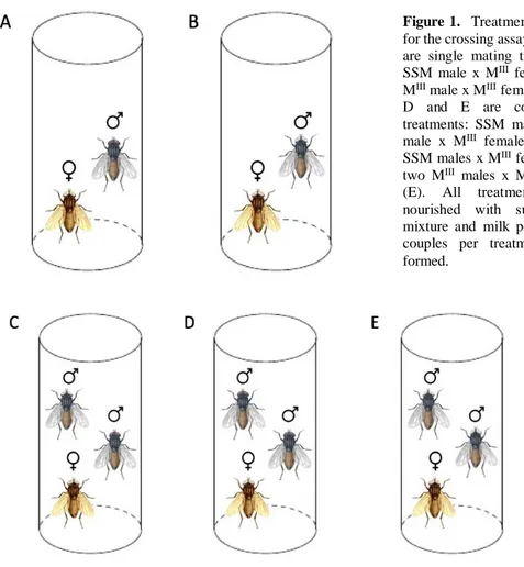
The experiment was design to allow Musca males to be put in a direct competition scenario and to compare different fitness components. Five treatments were created to establish both single mating and competition scenarios inter and intra-strain (Figure 1). Treatments A and B correspond to single mating scenarios and C, D and E to competition scenarios. In order to make possible to distinguish phenotype per strain when counting offspring in treatment C, MIII females were used (SSM offspring
show the wild type phenotype while MIII offspring have white eyes and brown bodied females). MIII
females were also used in the rest of the treatments to standardize the experiment and allow comparisons between treatments. Three traits were measured to proxy male fitness: reproductive success (obtained by counting the offspring produced by each male); head width (detailed below); and longevity (number of days from emergence to death). 30 couples were formed per treatment however, the final sample sizes differed due to premature death or escape of the males/females (sample values on the results section).
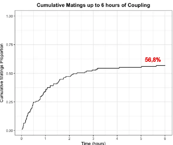
At the day of fly emergence, virgin males and females were separated and transferred to cups (density of 15 to 20 flies) nourished with milk powder and a continuous supply of sugar-water mixture. They were kept in these cups for 8-9 days so they could reach the age of maximum mating propensity (Hicks et al. 2004; plus personal observations). On the day of the experiment each male and female were transferred individually to a 100ml plastic tube (Figure 1). All tubes were then stored in the same climate room as in culture. After 48h, couples were separated (previous pilot studies showed a mating success rate over 50% after 6 hours – see Appendix, Figure 1; and personal observations indicated a close to
80% success rate after 24h). Males were transferred to individual tubes, again nourished with sugar-water mixture and milk powder and kept there until death to estimate longevity; females were transferred to egg laying cups (nourished with sugar-water mixture and milk powder) with a small recipient filled with food-mixture for egg posture. After 72h, the eggs were transferred to a culture beaker where more food mixture was added. RS was obtained by counting the offspring from each couple. In Treatment C, offspring from the SSM male was distinguished from MIII through the color of the eyes.
Multiple female assay
This assay was conducted in the same way as the “Fitness Assays”. On this assay however, only SSM flies were used and each male was allowed to couple with four different virgin females across 4 days (from 7 do 10 days old). The couples were paired for 24h before transferring the females to the egg laying cups and the males to the next tube with a new virgin female. The offspring was counted for each female and a final measure of male RS was obtained through the average of the four corresponding offsprings. Longevity and head width of each male were also measured.
Head Width measurements
All photos were taken with the males alive, so the longevity assays were not interrupted. In order to do this, the tubes were placed on ice for a few minutes to induce short-time paralysis. Then, the individuals were placed on a millimetric paper and three distinct photos were taken to each one of the males. The Fiji® software (Schindelin et al., 2012) was used to perform the head measurements on every photo. Three measurements were made per photo always establishing a new scale according to
Figure 1. Treatments created
for the crossing assay. A and B are single mating treatments: SSM male x MIII female (A);
MIII male x MIII female (B). C,
D and E are competition treatments: SSM male + MIII
male x MIII female (C); two
SSM males x MIII female (D);
two MIII males x MIII female
(E). All treatments were nourished with sugar-water mixture and milk powder. 30 couples per treatment were formed.
the millimetric paper. The average of the nine measurements was then calculated to establish the final HW value.
Statistical analysis
All plots, statistical tests and modelling were conducted under the R software® (version 3.4.2) (Team, 2014). The Shapiro-Wilk test was used to assess the data sets normality. The independent Mann-Whitney-Wilcoxon test and the unequal variances t-test were used to compare strains and competition scenarios between species. P-values lower than 0.05 were considered as statistically significant. The R packages used were ggplot2, ggpubr and tidyverse (Wickham, 2016) for the plots; ggpmisc to calculate the R2 values (Aphalo, 2016); and lme4 (Bates et al., 2015), lmerTest (Kuznetsova et al., 2017) and pscl
(Zeileis et al., 2008) for the modelling.
Results
Overall analysis
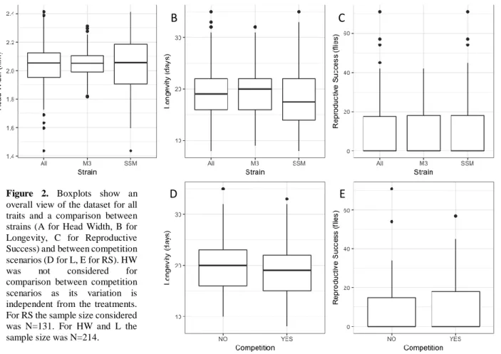
First, the whole data set was analyzed to look for differences between strains or competition scenarios. The sample size considered to analyze RS was N=131 and N=214 for HW and L. This difference in sample size is due to the inclusion of the “loser” male’s HW and L values in the competition treatments (C, D and E). “Loser” males did not have offspring and therefore no RS data points were considered whereas, HW and L could still be measured. The Mann-Whitney test showed no significant differences between strains for HW (p-value = 0.8232) and RS (p-value = 0.8255) (Figure 2A and 2C, respectively), and a significant difference was found for L (p-value = 0.0381) (Figure 2B). No significant differences were found between competition and non-competition scenarios for all traits (p-value = 0.1848 and Figure 2D for L; p-value = 0.146 and Figure 2E for RS).
A
B
C
E
D
Figure 2. Boxplots show an
overall view of the dataset for all traits and a comparison between strains (A for Head Width, B for Longevity, C for Reproductive Success) and between competition scenarios (D for L, E for RS). HW was not considered for comparison between competition scenarios as its variation is independent from the treatments. For RS the sample size considered was N=131. For HW and L the sample size was N=214.
Interactions between traits
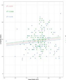
Each treatment was then analyzed to understand how the traits vary and interact with each other. An overall positive correlation is apparent between HW and L (Figure 3 - R2 = 0,012) - bigger
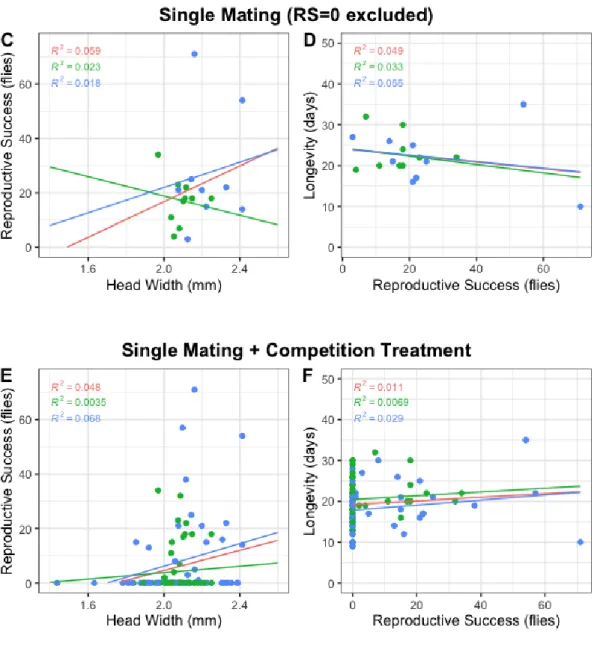
males tend to live longer. A quasipoisson model was fitted to the data, with L as dependent variable and HW as predictor variable (L ~ HW), however no significant effects were found. The single mating treatments (treatments A and B – N=53) showed a positive interaction between RS and both HW (R2 = 0,12) and
L (R2 = 0,016) (Figure 4A and 4B, respectively). Also,
the RS data appears to have a zero inflated distribution. In accordance to this, a zero-inflated negative binomial model was fitted to the data, with RS as dependent variable and HW and L as predictor variables (RS ~ HW + L). Then, this full model was compared to models in which either HW or L was removed as a predictor variable to estimate the correlation between L and these predictor variables (RS ~ HW vs. RS ~ HW + L and RS ~ L vs. RS ~ HW + L). HW (X2 =
7.4084; df = -2; p-value = 0.0246) had a significant effect on RS; and the effect of L (X2 = 5.4283; df =
-2; p-value = 0.0663) was almost significant. A model that included the interaction between HW and L as predictor variable did not show significance for any of the predictor variables (all values were obtained by comparing GLMs using lrtest() from the lmtest package (Zeileis and Hothorn, 2002)). Next, to discriminate for successful matings, data points on which RS=0 were removed (Figure 4C and 4D – N=19) – the overall RS-HW correlation stayed positive (R2 = 0,059) while the L-RS correlation turned
negative (R2 = 0,049). Lastly, if the competition treatment (treatment C) is added to the single mating
data, very similar correlations can be detected between RS and the other two traits (Figure 4E and 4F – N=103) – the correlation L-RS is a bit less accentuated though (Figure 4F). Again, a zero-inflated negative binomial model was fitted to this data, with RS as dependent variable and HW, L and the interaction between them as predictor variables (RS ~ HW + L + HW:L). This time however, no significant effects on RS were found for any of the traits nor the interaction.
Figure 3. Correlation between Head Width and
Longevity across the entire data set. MIII data
points are represented in green, SSM in blue and the orange slope contemplates both strains. All flies used in the experiment were considered (N=214).
Competition effect
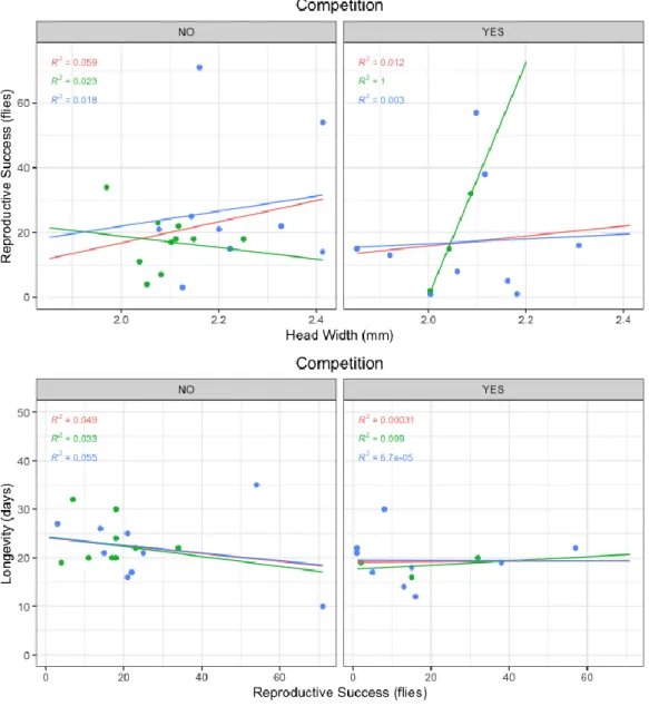
To further investigate how competition affects the studied traits, a comparison was made between the single mating treatments (A and B) and the mixed-strain treatment (C). The latter is the only competition treatment where a link between RS and the other traits could be made, as offspring could be attributed to the corresponding male parent (for intra-strain competition this distinction was not possible). In line with the previous Mann-Whitney test, no observable differences could be detected between competition scenarios (Appendix, Figure 2). Even though the plot suggests a positive correlation between RS and HW for the MIII flies (R2 = 1), the very low sample (only 3 data points)
discredits this as a relevant result. When looking at the winners vs. losers’ direct comparison, no clear patterns can be detected (Figure 5). Most winners are SSM and bigger, while half of the winners lived
Figure 4. Correlation between Reproductive Success and Head Width (graphs on the left column) or
Longevity (graphs on the right column). A+B (N=53) refer to the single mating dataset (including treatments A and B). C+D (N=19) refer to the same dataset with the exclusion of points on which RS=0. E+F (N=103) refer to the initial single mating dataset with the addition of the data from treatment C. Each strain’s data points were represented with one color (green for MIII and blue for SSM) and a slope that contemplates both
longer/shorter than the losers, although the low sample (N=12 data points in total) does not allow for significant conclusions to be made. Mann-Whitney tests did not find significant differences between winners and losers for both traits.
Multiple female experiment
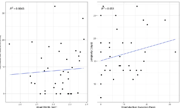
When analyzing the average RS for each male across the 4 days (N=39), the same patterns as the ones observed on the previous experiment emerged (the average RS of the 4 days was used to proxy individual male RS). There seems to exist a slightly positive correlation between RS and HW (R2 =
0,004). There is the same correlation but more accentuated between L and RS (R2 = 0,051) (Appendix,
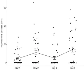
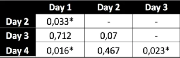
Figure 3). A zero-inflated negative binomial model was fitted to the data, with RS as dependent variable and HW, L and the interaction between them as predictor variables (RS ~ HW + L + HW:L). No significant effects on RS were found for any of the traits nor the interaction between them. An interesting detail was detected about this dataset: the male RS seems to fluctuate across time, with lower values on days 1 and 3 and higher values on days 2 and 4 (Figure 5). These differences were found to be significant when performing a pairwise t-test with no assumption of equal variances (Table 1). A Levene’s test was used to confirm the lack of homogeneity of variances (p-value = 0.0026) (obtained by using leveneTest() from the car package (Fox and Weisberg, 2019)). There is no visible pattern for individual RS variation across days (Appendix, Figure 4).
Figure 5. HW (A) and L
(B) direct comparison between winners and losers on treatment C (competition inter-strains). Plots are sorted first, by strain; and then by descending net difference (with the bigger differences starting on the left). Winner’s trait score is marked in green while the loser’s is in red. Each pair of males is identified on the x axis accordingly to its treatment tube.
Figure 6. (A) Male reproductive success scored
across 4 days (N=39). Data points plotted per day with respective average also represented. On each day the same male was coupled with a different female, and the resultant offspring was counted. (B) Table for RS values across time. First row indicates average RS per male; second row indicates total offspring per day (sum of every male’s RS); and third row indicates the percentages of the total RS after 4
Discussion
A novel experimental design to measure fitness
Male and female fitness have often been associated with each other, painting a story of conflictual coevolution (Arnqvist and Nilsson, 2000; Birkhead and Pizzari, 2002; Chapman et al., 2003; Cordero and Eberhard, 2003; Innocenti and Morrow, 2010). In order to understand such processes, one must find the bridge between fitness and the genetic basis of SA. With this experiment, we built the foundations for a flexible experimental design that allows the measurement of several components of fitness (both in males and females) under different scenarios. This study incorporated: two different strains; two different competition scenarios; and the measurement of three components of fitness. It successfully allowed for a transversal comparison between strains, competition treatments and traits. This design would also be suitable for other comparisons - more strains can be included, as well as different treatments (more competition scenarios or treatments with other types of variation – per example: changes in temperature, nutrition, individual age or number of total individuals per treatment) – hence its flexibility. The changes would depend on the goals of potential studies: Scoring mating success per example, would allow to distinguish males that did not fertilize any female from males that mated but did not generate any offspring (this distinction is explained with more detail on the next paragraph); Offspring viability could also be included on this experimental design without any methodological impediment and it would theoretically serve as a good fitness proxy (Pekkala et al., 2011). It could be added to the list of traits to increase the correlation analysis. However, one should be careful when trying to estimate individual fitness from offspring viability. If attributed to one of the parents, it would under-estimate the effect of the actual parental traits on fitness (exceptions in case of pleiotropic effects or linkage disequilibrium between parental and offspring genes) (Fedorka and Mousseau, 2004; Hunt and Hodgson, 2010); and as last example, it would also be easy to score the offspring’s sex ratio. As previously mentioned, the sex ratio of a population has a significant impact on male-male competition and on female’s reproduction costs (in the case of Musca) and its effect on the evolution of sexual organisms should be considered (Uller et al., 2007; Carrillo et al., 2012; Booksmythe et al., 2017; O´Brien et al., 2018). Sex ratio will affect the evolutionary dynamics of a population and can show interesting interactions with other components of individual fitness.
A change worth to be considered is the addition of video recordings. If performed with the adequate equipment it could considerably improve the methodology. Musca copulations are considerably long – from 40min to 1h30min (Leopold, Terranova and Swilley, 1971; Andres and Arnqvist, 2001; plus personal observations), and it could take several hours for a couple to start mating (see Appendix – Figure 1). To have a reliable estimate of the number of successful matings one must have a recording set that allows for longer recordings that can also be extended during night time (with no luminosity). In our experiment, recordings longer than 6h were not possible, which only gives an idea about the potential mating rate across the 24h of coupling (Appendix – Figure 1). The scoring of
Table 1. Pairwise t-test with no assumption of
equal variances between RS across different days. P-values lower than 0.05 were considered as statistically significant.
successful matings per male/female is actually a powerful measurement, as it would allow the distinction between RS=0 cases on which no mating occurred, from RS=0 cases on which the male successfully engaged the female. Such distinction would mean different degrees of fitness for the males – if a male does not engage the female or fails on its courtship this could probably be considered low fitness due to sexual selection mediated by female choice; by the other hand, if the transfer of semen was apparently successful, the measurement of male fitness gets more complicated. It could be that some kind of cryptic female choice is in play (reviewed by Firman et al., 2017) or that the female could not produce offspring by its own fault (low female fitness). The recording of the copulations would also allow for the examination of mating patterns and could even account for the transfer of seminal fluids. In Musca, full sperm transfer is achieved in approximately 10 minutes (Murvosh et al., 1964), and the accessory seminal substances (responsible for increasing oviposition rate and inhibiting females from remating) are transferred after 40 minutes (Arnqvist and Andrés, 2006). If a male only transfers the semen without the seminal fluids this would have impact on the fitness of both the male and the female (Riemann and Thorson, 1969; Hicks et al., 2004; Arnqvist and Andrés, 2006) and should be considered on the final net fitness sum under consideration. Longer video recordings would add a new layer of detail to our male fitness characterization and could also be useful when studying female fitness.
Overall, this design has proven to be a solid approach to fitness assays in Musca domestica and can be adjusted according to the main goals of the study.
The collected data
On the study performed, the small sample collected does not allow for major conclusions about the interactions between fitness traits to be made. Nonetheless, information about each trait can still be considered, and the results allowed for some guidelines to be established when analyzing interactions between male fitness traits. The lack of differences between strains for neither of the traits (Figure 2A-C) is a good indicator that fitness can be compared between these two strains. There was the one exception of longevity that showed a significant difference between SSM and MIII (even if almost not
significant – p-value = 0,03808). This difference is probably caused by the higher variance observed for SSM (Figure 2B) which makes sense since SSM flies come from an outbred population compared to MIII, that is a largely isogenic lab strain (see Materials and Methods). Moreover, no significant
differences were found when comparing the RS of SSM males when they mate with MIII or SSM females
(results obtained through comparing Treatment A (Figure 1) with the Multiple Female experiment data set). The transversal lack of differences between strains suggests that MIII can successfully be used as a
mutant strain on this type of comparative studies.
Between competition treatments the outcome was the same – no significant differences were found (Figures 2D and 2E). Having single mating or two males for one female seems to have no effect both on RS and L (HW is by definition not affected by competition). This result was not expected since competition seems to have a big effect on Musca fitness, particularly in males. The low sample size obtained for RS on the competition treatment (n=25; and only 12 data points on which RS>0) may explain the lack of differences. It is also a hypothesis that relaxed selection causes a decrease on the flies’ competitive ability. This is characteristic of long-established laboratory populations (such as the ones used on this study) and has been reported both in Drosophila (Shabalina et al., 1997) and Musca (Bryant and Reed, 1999). The existence of enough females for every male to mate and the continuous availability of food and water is naturally expected to reduce selection pressures (Coss, 1999). As a result of this, the impact of competition on the passing of genes to the next generation in diminished and the fitness differences between flies that compete and not compete starts to disappear. Nonetheless, a bigger sample size is needed to fully understand if direct competition between males affects the offspring produced. When looking at longevity, the sample size is more considerable (N=214). The results,
however, did not align with our expectations. Previous literature has suggested that a decrease on longevity should be a natural consequence of higher activity rates and reproduction-related physiological costs (Ragland and Sohal, 1973; Hicks, Hagenbuch and Meffert, 2004; Barnes et al., 2008; reviewed by Speakman, 2005). As such, competition should be a natural depressor of longevity with more competing scenarios having short-living males. In this study, even though competing males have a lower L average than non-competing ones (Figure 2D), this difference was not significant. The same goes for the interaction between HW and L: there is a slight indication of a positive correlation that is not significant (Figure 3). The lack of significance in both cases can probably be explained by the aforementioned decrease of aggressive/competitive behavior due to relaxed selection. Less competitivity should cause a standardization of the population and diminish the impact of competitive elements and/or allocation of resources on longevity. The differences in longevity between competition scenarios and its correlation with body size would then be attenuated.
Something noticeable about the data set is the abundance of null reproductive success (RS=0). This could mean either low female fitness – females were unable to produce offspring; or low male fitness – males did not fecund the females successfully or mating did not occur at all (the scientific meaning of this distinction is detailed on the previous paragraph). Low reproductive success was here interpreted as an indicator of low fitness for males even with a certain degree of error derived from the contribution of female fitness to the offspring size. Again, this degree of error could be diminished if mating success could be scored and null RS scores could be related to sex-specific low fitness. Still, the big amount of RS=0 cases across both the Crossing Fitness Assay and the Multiple Female Assay goes in line with the parallel experiment (Appendix – Figure 1) that showed that only 56,8% of the established couple’s mate after 6h. A low mating rate could imply a sub-optimal methodology that does not assure fertilization. Although, several adjustments were made across pilot studies to achieve the highest possible mating success rate in the final assays here presented: No CO2 was used when forming the
couples; all flies were 7-10 days old to assure maximum mating propensity (Hicks, Hagenbuch and Meffert, 2004; plus personal observations); all experiments were initiated in the afternoon as flies show higher activity during the latest hours of light (due to personal observations and also noticed for other dipterans - Sakai and Ishida, 2001); couples were kept together for at least 24h to capture the entire circadian cycle. To interpret the majority of couples with zero offspring we should first note that in terms of fitness, it is not the absolute value but the relative measurement that serves as stronger determinant (Orr, 2009; Hunt and Hodgson, 2010). For our case, this means that being able to produce offspring – even in low numbers – can pose as a big fitness advantage considering that a big part of the matings result in zero offspring. Then, it is also important to remember that mating behavior can be strongly modulated by the social context (Laturney and Billeter, 2014). In Drosophila it has been showed that mating rates increase with group size (Laturney et al., 2018) and group diversity (Billeter et al., 2012) suggesting that the measurement of RS on our experiments can indeed be affected by the way flies were paired to mate. This method constitutes the normal paradigm in laboratory, although it diverges from the natural mating behaviors observed in nature. For Musca, mating normally occurs within a group that is occupying a food source (Scott and Lettig, 1962). Thus, cases where every individual only has one single encounter with the opposite sex are very unlikely to happen if not in laboratory conditions. In nature, each fly has the opportunity of mating several times and with different partners which may affect the offspring produced. At the end of the day, we have to rely on the results generated by this kind of studies to inform us about the processes of reproduction and in our case, to measure fitness. One should always take social context into consideration and, even though is not clear how much it explains the abundance of RS=0 cases, it most likely affected our results.