* Corresponding author: E-mail: [email protected] Received: April 25, 2018
Approved: August 29, 2018
How to cite: Somavilla A, Gubiani PI, Zwirtz AL. Tipping bucket prototype for automatic
quantification of surface runoff
rate in plots. Rev Bras Cienc Solo. 2019;43:e0180096.
https://doi.org/10.1590/18069657rbcs20180096
Copyright: This is an open-access article distributed under the terms of the Creative Commons Attribution License, which permits unrestricted use, distribution, and reproduction in any medium, provided that the original author and source are credited.
Tipping Bucket Prototype for
Automatic Quantification of Surface
Runoff Rate in Plots
André Somavilla(1)
, Paulo Ivonir Gubiani(1)* and Anderson Luiz Zwirtz(2) (1)
Universidade Federal de Santa Maria, Centro de Ciências Rurais, Departamento de Solos, Santa Maria, Rio Grande do Sul, Brasil.
(2)
Instituto Federal de Santa Catarina, Área de Recursos Naturais-Produção Vegetal, Campus São Miguel do
Oeste, Santa Catarina, Brasil.
ABSTRACT: Quantification of runoff rate is an onerous task with non-automated devices;
it requires a lot of manual labor to perform measurements. In this study, an automatic
device to quantify the surface runoff rate from plots with a small area was developed
and tested. The prototype was based on the tipping bucket technique and built with reused materials. Its performance was tested in the laboratory and a calibration curve was developed to improve measurement accuracy. The device can be used for
automatic quantification of surface runoff in small plots, with a flow rate of less than
750 × 103 mm3 min-1. The device can be built with different dimensions to measure different flow rates. In that case, the error measurements and calibration curve must
be recalculated.
Keywords: tipping bucket, Gauge, flow rate, watershed.
INTRODUCTION
Runoff has been studied for several purposes, mainly to quantify erosion processes
and soil and nutrient losses (Panachuki et al., 2011; Oliveira et al., 2013; Costa and
Rodrigues, 2015). Surface runoff models and soil water infiltration models (Spohr et al.,
2009; Abrantes et al., 2015) have been developed and evaluated.
In scenarios of either natural or simulated rainfall, flow rate from a single channel or a collection of channels needs to be measured to quantify runoff. The total runoff volume (Costa et al., 2013; Costa and Rodrigues, 2015) and the surface runoff rate (Spohr et al., 2009; Oliveira et al., 2013; Lima et al., 2015) are the main variables used to express runoff. Runoff quantification can be a laborious time-consuming task, especially when the runoff rate is quantified with non-automated devices. In studies on a watershed scale, the runoff discharged into a river changes its water level. This change is detected by a limnigraph and converted into runoff with the aid of a calibration curve (Almeida et al.,
2013; Rodrigues et al., 2013). In soil plots, the limnigraph is not an appropriate device,
so runoff measurements are usually performed by collecting either all or an aliquot of the outflow at a given time interval, which is then measured using scaled containers (Oliveira et al., 2013; Lima et al., 2015). This runoff measurement strategy cuts down on the need for manual labor by obtaining runoff rates at discrete times, mainly from long
rainfall events. Furthermore, an unexperienced researcher can inadvertently introduce
many errors when quantifying runoff. Therefore, the use of automated devices to quantify plot outflow can minimize these problems.
The tipping bucket technique is widely used to measure rainfall rate (Fankhauser, 1997).
This technique can also be used to measure other flows, as proposed by Edwards et al. (1974) for quantification of surface runoff in plots of up to five hectares. Nevertheless, there is no tipping bucket configured to accurately measure runoff in plots on a square
meter scale. Thus, in this study we sought to develop and test an automated tipping
bucket to quantify the surface runoff rate from plots with small area.
MATERIALS AND METHODS
The tipping bucket prototype was made at the Soil Physics Laboratory of the Federal University of Santa Maria (UFSM) – Rio Grande do Sul, Brazil. The gauge system was molded from a rectangular metal sheet 120 × 110 mm (Figure 1); its length was 2.75 times its width (110 mm long, 40 mm wide, and 40 mm high). A metal wall was inserted
at the center of the gauge (55 mm), separating two sections of equal volume. A fixed
metal axis was attached at the gauge center and a stem containing a magnet at the top was attached to one side.
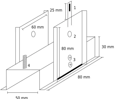
The tipping bucket system was then attached to a metal base composed of two parallel metal sheets (80 mm high and 60 mm wide) and an inverted metal channel (80 mm length, 50 mm wide, and 30 mm high). In construction of the metal base, the plates were secured at one end by the metal channel (Figure 2) and, at the other end, openings were made for coupling the tipping system.
To count the see-saw movements of the tipping system, a Reed Switch magnetic sensor was attached at the top of one of the parallel sheets (Figure 2) so that its position
coincided with the magnet fixed on the tipping scale. Thus, when the scale is moved,
the magnet (Figure 1) causes excitation in the magnetic sensor (Figure 2) and a pulse of energy is generated and transmitted to the reading and data storage system (CR1000
datalogger, Campbell Scientific, Inc., Logan, UT, USA).
collected water into the gauge. An epoxy resin was used to reduce the funnel outlet
opening to a 3.4 mm diameter, improving the direction of water flow into the gauge
system and restricting very high volumes. A nylon mesh was attached onto the top of the funnel to prevent the input of coarse material. The fully assembled device is
shown in figure 3.
The water volume required to set the gauge system in motion was adjusted after the system had been installed inside the PVC pipe. Due to the capacity of the system, the water volume was adjusted to 15 × 103 mm3, using the adjusting bolts (Figure 2), for both halves of the gauge. Possible errors include not only those from the adjustment of water volume, but also errors in the readings performed by the device, such as errors
40 mm
110 mm Magnet
40 mm
Fixed axis
Figure 1. Diagram of the tipping bucket system.
Figure 2. Diagram of the metal base used to support the tipping bucket system.
30 mm
80 mm 3
2
4
80 mm 60 mm
50 mm
25 mm 1
arising from the turbulent flow of water within the gauge and the period necessary for the tipping “seesaw” cycle, resulting in larger errors for measurements of larger flows
(Edwards et al., 1974). Therefore, Edwards et al. (1974) and Calder and Kidd (1978) suggest a correction in the readings performed by the tipping bucket device.
The need to correct the readings was verified in the laboratory, and a calibration curve was generated by relating the added measured flow rate for each tipping interval (Δt, min) of 1 min to the flow rate estimated by the device for the same interval. For this purpose, nine flow rates in the range of 0.045 to 2.5 mm3 min-1 were obtained and maintained constant along the Δt interval by means of maintaining the water level inside the funnel constant. As the error from device estimates is dependent on changes in flow rate along the Δt interval and the magnitude of Δt (Edwards et al., 1974), the calibration curve was tested against two Δt (0.16 and 1 min), in which the flow rates randomly varied along the Δt interval.
The performance of the calibration curve at each Δt interval was evaluated by the Nash-Sutcliffe Efficiency (NSE) (Equation 1), which determines the magnitude of the residual variance, indicating how much the added flow rate versus estimated flow
deviates from the 1:1 line (Moriasi et al., 2007).
NSE = 1 –
Σ
n i=1 (Yi
ad – Yi
est )2
Σ
n i=1 (Yiad – Ymean
)2
Eq. 1
in which: n is the number of evaluations; Yi est
is the estimated flow rate by the device;
Yi
ad is the added flow rate; and Ymean is the mean of the added flow rate.
The NSE values range between -∞ and 1, with NSE = 1 being the optimal value. Values
between zero and 1 are considered indicators of adequate performance, while values below zero represent inadequate performance.
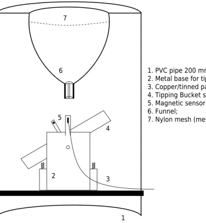
Figure 3. Vertical cross-section of the automatic runoff-measuring device. 7
6
5
4
3
1
1. PVC pipe 200 mm;
2. Metal base for tipping bucket system; 3. Copper/tinned parallel cable;
4. Tipping Bucket system;
5. Magnetic sensor Reed Switch + magnet; 6. Funnel;
7. Nylon mesh (mesh of 3 mm).
The percentage of bias (PBIAS) (Equation 2) was also used, which shows the trend of the
added flow rate to be larger or smaller than the estimated flow rate (Moriasi et al., 2007):
PBIAS =
Σ
n i=1 (Yiad – Yi
est )(100)
Σ
n i=1 (Yiad )
Eq. 2
The optimal value for PBIAS is zero. Positive values indicate underestimation, and negative
values indicate overestimation of estimated flow rate in relation to added flow rate.
Another possible error arises from the fact that 15 × 103 mm3 of water must be stored so that the gauge starts the water unloading movement. If this volume is not accumulated inside the gauge, the water fraction below 15 × 103 mm3 will not be quantified, resulting in a resolution error. For that reason, numerical analysis was performed to quantify the
importance of resolution error on the measured flow.
RESULTS AND DISCUSSION
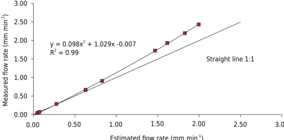
From visual analysis of the results, it can be observed that the relation between the
measured flow rate and the estimated flow rate by the device with Δt of 1 min departs from the 1:1 line, confirming the need for calibration. The calibration curve was generated by using a quadratic function, which related the added flow rate to the estimated flow
rate with a R2 of 0.99 (Figure 4).
The performance of the quadratic calibration curve generated from Δt of 1 min was considered satisfactory in prediction of the flow rate for Δt of 0.16 and 1 min, according to the NSE and PBIAS coefficients (Table 1). Despite the small variation in NSE and
PBIAS, the best calibration curve performance, for both NSE (values close to one)
and PBIAS (values close to zero), was observed for Δt of 1 min. Both NSE and PBIAS
indicated that there was underestimation (positive values), but the underestimation was less than 3 %.
The calibration curve generated does not take into account the effect of sediment concentration in the water flow. The presence of sediments increases the density of the fluid, requiring a lower volume of fluid to promote the seesaw movement of the gauge,
which may cause an overestimation of the error. If necessary, users must check and
change the calibration curve when sediments are present in the discharge flow.
y = 0.098x2 + 1.029x -0.007 R2 = 0.99
0.00 0.50 1.00 1.50 2.00 2.50 3.00
0.00
Measured flow rate (mm min
-1 )
Estimated flow rate (mm min-1)
Straight line 1:1
3.00 2.50
2.00 1.50
1.00 0.50
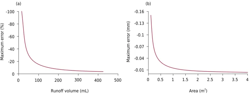
The device resolution error occurs only once during the runoff event and its magnitude is dependent on both the runoff volume and the plot area. In this study, plot means a theoretical surface used for mathematically evaluating the effect of the surface size on water accumulation and resolution error. Smaller runoff volume and smaller plot surface area result in greater participation of the error in the reading, as shown in figures 5a and 5b, respectively. The percent of error increases as runoff volume decreases, because this increases the proportion of the water not unloaded from tipping at the end of discharge flow (if there is not sufficient water accumulated to promote the “seesaw” movement) in relation to total discharge flow. Reduction in plot surface area also decreases total runoff volume; therefore, the effect is the same. The maximum rate quantified in this study was 750 × 103 mm3 min-1 in measurements performed in the laboratory and with the device described above. Although there is an inverse relation between resolution error and plot area, for good performance of the
device, the plot area must have a flow rate of less than 750 × 103 mm3 min-1. If the flow rate exceeds 750 × 103 mm3 min-1 the device should be built in larger dimensions.
This device is inexpensive and can be easily assembled. Among the materials used, the CR1000 datalogger is the costliest acquisition. However, it may be replaced by another data storage device, without compromising performance.
CONCLUSION
This tipping bucket prototype can be used for automatic quantification of surface runoff in plots with a flow rate of less than 750 × 103 mm3 min-1.
To obtain satisfactory approximation of real values, a calibration curve must be used.
The dimensions and capacity of the device can be adapted according to the needs of each user; however, the error analysis and the calibration curve must be recalculated.
Table 1. Performance of the device calibration curve (n=4)
Δt(1) NSE(2) PBIAS(3)
min %
0.166 0.992 2.732
1.000 0.997 2.274
(1) Tipping interval (Δt). (2) Nash-Sutcliffe Efficiency (NSE). (3)
Percentage of bias (PBIAS).
Figure 5. Maximum resolution error by runoff volume (a) and plot area (b). Negative values indicate underestimation of flow rate. -100
-80
-60
-40
-20
0 0
Maximum error (%)
Runoff volume (mL)
-0.16
-0.13
-0.1
-0.07
-0.04
-0.01
0
Maximum error (mm)
Area (m2)
(a) (b)
500 400
300 200
REFERENCES
Abrantes JRCB, Lima JLMP, Montenegro AAA. Desempenho da modelagem cinemática do
escoamento superficial para chuvas intermitentes em solos com cobertura morta. Rev Bras Eng
Agric Ambient. 2015;19:166-72. https://doi.org/10.1590/1807-1929/agriambi.v19n2p166-172
Almeida AQ, Ribeiro A, Leite FP. Modelagem do balanço hídrico em microbacia cultivada com
plantio comercial de Eucalyptus grandis X urophylla no leste de Minas Gerais, Brasil. Rev
Arvore. 2013;37:547-56. https://doi.org/10.1590/S0100-67622013000300018
Calder IR, Kidd CHR. A note on the dynamic calibration of tipping-bucket gauges. J Hydrol. 1978;39:383-6. https://doi.org/10.1016/0022-1694(78)90013-6
Costa CFG, Figueiredo RO, Oliveira FA, Santos IPO. Escoamento superficial em Latossolo Amarelo distrófico típico sob diferentes agroecossistemas no nordeste paraense. R Bras Eng
Agric Ambiental. 2013;17:162-9. http://dx.doi.org/10.1590/S1415-43662013000200007
Costa YT, Rodrigues SC. Relação entre cobertura vegetal e erosão em parcelas representativas de cerrado. Rev Geogr Academica. 2015;9:61-75. https://doi.org/10.18227/1678-7226rga.v9i2.3160
Edwards IJ, Jackon WD, Fleming PM. Tipping bucket gauges for measuring
run-off from experimental plots. Agr Meteorol. 1974;13:189-201.
https://doi.org/10.1016/0002-1571(74)90046-6
Fankhauser R. Measurement properties of tipping bucket rain gauges and
their influence on brain runoff simulation. Water Sci Technol. 1997;36:7-12.
https://doi.org/10.1016/S0273-1223(97)00625-2
Lima CA, Montenegro AAA, Santos TEM, Andrade EM, Monteiro ALN. Práticas agrícolas no cultivo
da mandioca e suas relações com o escoamento superficial, perdas de solo e água. Rev Cien
Agron. 2015;46:697-706. https://doi.org/10.5935/1806-6690.20150056
Moriasi DN, Arnold JG, Van Liew MW, Bingner RL, Harmel RD, Veith TL. Model evaluation
guidelines for systematic quantification of accuracy in watershed simulations. ASABE.
2007;50:885-900. https://doi.org/10.13031/2013.23153
Oliveira ZB, Carlesso R, Martins JD, Knies AE, Dalla Santa C. Perdas de água por escoamento
superficial a partir de diferentes intensidades de chuvas simuladas. Irriga. 2013;18:415-25.
https://doi.org/10.15809/irriga.2013v18n3p415
Panachuki E, Bertol I, Alves Sobrinho T, Oliveira PTS, Rodrigues DBB. Perdas de solo e de água
e infiltração de água em Latossolo Vermelho sob sistemas de manejo. Rev Bras Cienc Solo.
2011;35:1777-85. https://doi.org/10.1590/S0100-06832011000500032
Rodrigues JO, Andrade EM, Mendonça LAR, Araújo JC, Palácio HAQ, Araújo EM. Respostas hidrológicas em pequenas bacias na região semiárida em função do uso do solo. R Bras Eng Agric Ambient. 2013;17:312-8. https://doi.org/10.1590/S1415-43662013000300010
Spohr RB, Carlesso R, Gallárreta CG, Préchac FG, Petillo MG. Modelagem do escoamento
superficial a partir das características físicas de alguns solos do Uruguai. Cienc Rural.