Multivariate unit root tests

i

_~DAÇÃO

GE7VUO VARGAS

Praia de Botafogo, nO 190/10° andar - Rio de Janeiro - 22253-9110

Seminários de Pesquisa Econômica 11 (2

a

parte)

II

MULTIV ARIATE UNIT

ROOT TESTS

11

RENATO FLÔRES

(EPGE-FGV / Fac. de Direito-UFRJ / ULB)

MULTIVARIATE UNIT ROOT TESTING

Renato G. Flôres Jr, Pierre-Yves Preumont and Ariane Szafarz

CEME, Université Libre de Bruxelles

Abstract

A new multivariate test for the detection ofunit roots is proposed. Use is made ofthe possible correlations between the disturbances of difIerent series, and constrained and unconstrained SURE estimators are employed. The corresponding asymptotic

distributions, for the case oftwo series, are obtained and a table with criticai vaIues is generated. Some simulations indivate that the procedure performs better

than

the existing aIternatives.

Apri11995

[ Attention: This is a very preliminary version to serve as supporting material to the seminar, please do not quote. ]

I. INTRODUCTION.

Since Dickey and Fuller (1979, 1981)'s benchmark contribution, many papers have stressed the statistical problems related to unit root tests. Phillips and Perron (1988) and Ng and Perron (1994) are only two examples of attempts to shed some light on unwanted behaviour - under different settings - and of corrections or new procedures to deal with them. Given the considerable diversity of the altemative hypotheses this is not an easy task, and sometimes general statements - not very encouraging for the daily practitionner - are produced. As an example, there is fairly general agreement that moving averages are the most dangerous altematives. However, though Hall (1989)'s suggestion theoretically solves the problem, the issue of identifying in practice the existence of the moving average remains open. Moreover, as unit root tests are a prerequisite for other procedures, like cointegration testing. this lack of power may create an embarrassing pre-testing bias (see, for instance, Elliot (1993)).

In all the studies up to now attention has been centred on the case of one series. However, the need to perform the test on a group of series closely related, like exchange-rates for several currencies, or basic macroeconomic indexes, calls for a multivariate approach to the problem. Indeed, one could take advantage of the correlations between the residuaIs in the different series and, like in Zellner (1962)'s pioneering article, improve the efficiency of the estimators and tests. Abuaf and Jorion (1990) have followed this direction, in the context of real exchange rate series. They improved the estimation of the autocorrelation coefficients though constraining a common dynamics under the null. Quah (1992) and Levin and Lin (1993) have approached the probIem in a somewhat different way, viewing the multivariate framework as a panel structure in which at Ieast one of the dimensions goes to infinity.

In this paper we develop multivariate testing procedures generalising Abuaf and Jorion (1990)'s idea. The cases of a "common" unit root and of different nonstationary/stationary behaviour are addressed and the asymptotic distributions are found. CriticaI vaIues for the case of two series are presented, and some preliminary simulations point favourably to the proposed tests.

The general model and related tests are discussed in the next section. CriticaI values and simulations are presented in Section 3, while Section 4 concludes. The derivations of the limit distributions is presented in an Appendix.

11. THE MODEL AND THE TESTS.

We consider the following set of series:

where the vector process {'Ut }

= {(

'Uit)} satisfies the hypotheses in Phillips and Solo (1992).

Several hypotheses of the form :

HO:ai = 1 for i E I (I c {l, ... ,p}), ai < 1 for i E IC (2.1 ) can be of interest. In particular, the case:

HO:ai =1, ISiSp, (2.2)

imposes a common I( 1) dynamics to all series.

We shall consider tests of the above unit root hypotheses in which the autoregressive coefficients are estimated by means of Zellner's SURE method. The equalities present either in (2.1) or (2.2) can be taken into account or not in the estimation procedure, giving rise to what we shall call constrained and unconstrained tests. The former, in the case (2.2), have been proposed and numerically studied by Abuaf and Jorion (1990) and will be called the AJ test.

If the parameter a = (ai) is estimated by the method SURE. then (2.2) represents a limit situation in which the equalities in the null may be fully used. However, rejection of the null may have many forms; actually, any of those represented in(2.1).

Our procedure starts then with the stronger condition (2.2). As wiU be seen in the next section, this does not necessarily imply that the constrained AJ test should be used. If the null is rejected, inspection of the estimated ai may help in choosing an appropriate version of (2.1) as the new nu I!. In this case, the fact that some {Xit} series are stationary is crucial and may greatly improve the results. Adequate testing of (possible) successive steps may eventually lead to a final structure of stationary and

non-stationary series. This can produce a feasible methodology even for moderately high values of p.

The asymptotic distributions for the three types of tests, when p=2, are now presented. AlI proofs are given in the Appendix.

Consider the bivariate model :

xo

=

yo

=

0,

(2.3)

where {[ u_t v

d '}

is an i.i.d. zero mean process2, with a regular variance-covariance

t>O

matrix

n,

given by:

n=[O'II O'I2J,

0'12 0'22

and the corresponding correlation is

(2.4)

(2.5)

Let us suppose first that

n

is known. The following tests are the bivariate versions of (2.2) and (2.1), respectively :

(2.6)

and

(2.7)

Hypothesis Hbl) can be dealt with in two different ways. We shall first discuss the distribution of the test statistic numerically studied by Abuaf and Jorion (1990), in which the equa1ity constraint is used for estimating the autoregressive coefficient. Then. hypothesis Hg) will be studied under an unconstrained SURE estimator.

As proved in the Appendix, the limit distribution of the AJ test 1S:

\vhere {W U(S)}SE[O.1] and {W y(s)}SE[O,I] are standard brownian motions associated

respectively to { Ut

1

et { v t } .

-valI

J

-Ja22

Formula (2.8) shows that only the correlation coefficient appears in the limit distribution. This means that if the unknown variances are estimated in a consistent way. this limit wiU be unchanged.

Two extreme cases should be mentioned. On the one hand. if PI2 = 0, i.e. no advantage exists in the SURE procedure, an expression close to the DF classical test is found: I I fWu(s)dWu(s)+ fWy(s)dWy(s) T(â-1)=>o O }

(\V~

(s) +

W~

(s) )dS O

*(W~(l)+W~(l))-l

-

.,:-;.---

}(W~

(s) +

W~(s)

)ds O (2.9)

On the other hand, when PI2 -7 1, expression (2.8) tends to :

(2.10)

what should really be taken as a limit case, since, if PI2

=

1, the variance-covariance matrix

n

is not invertib1e.

If unconstrained SURE estimation is used under hypothesis

Hb

l), the limit distribution of the estimator of the autoregressive coefficient aI in (2.3), for instance, will be:

If P12 = 0, we have exactly the Dickey-Fuller statistic :

1

fW

v dW u T(ci-I)

=>7?---f

W~

(s)ds O (2.11 )

We now consider hypothesis

Hb

2). The asymptotic distribution for T(ci_l -I) will be :

1 I

fW

u(s)dW u(s) - P12

fW

u (s)dW y(s)

O O

1

f

W~(s)ds

O

(2.12)

The Dickey-Fuller statistic is again found if PI2 = 0, while the case when

PI2 ~ 1 would give the maximal gain achieved from the correlation between the disturbances. This limit expression is :

1 1

fW

u (s)dW u (s) -

fW

u (s)dW y(s) O O 1

f

W~(s)ds

O (2.13)

Notice that the distribution in (2.13) is independent of the true a2 value, only its stationarity being re1evant. This means that, for sufficiently large samples, tables of

criticaI vaIues do not need to take into account this parameter. Actually, the stationary coefficient "helps" in weakening the influence of the (other) non-stationary series. To illustrate this statement, consider the model:

{

Xt = xt-I + ut

I I

where:E[ut,Vf]=Õu,·k

Yt = a2Yt-1 + Vt' a2 < 1

One can successively write :

t-I cov(xt ,Yt)=a2 cov(Xt_I,Yt_d+k=a~ cov(xO,Yo)+k

I

a2.

i=O

so that as t ---7 00 the covariance approaches the finite value k. 1 _.

l-ai

(2.14)

The results In this section emphasize that the corelations between the disturbances of the series of interest play a crucial role. UnfortunateIy, these correlations are unknown in the majority of the practical cases. Nevertheless, as with the feasible SURE, use of a consistent estimator for them guarantees the good properties of the theoretical test statistics. This issue is further supported in the next section.

IH. MONTE CARLO RESULTS

3.1. Criticai Values.

In order to have an idea of the behaviour of the proposed tests we have first compared the univariate use of the DF test with the following possibilities :

i) the AJ procedure with known and unknown correlation (to be called AJK and AJU. respectively);

ii) the non-constrained approach to (2.2) with known and unknown correlation (to be called MK and MU, respectively).

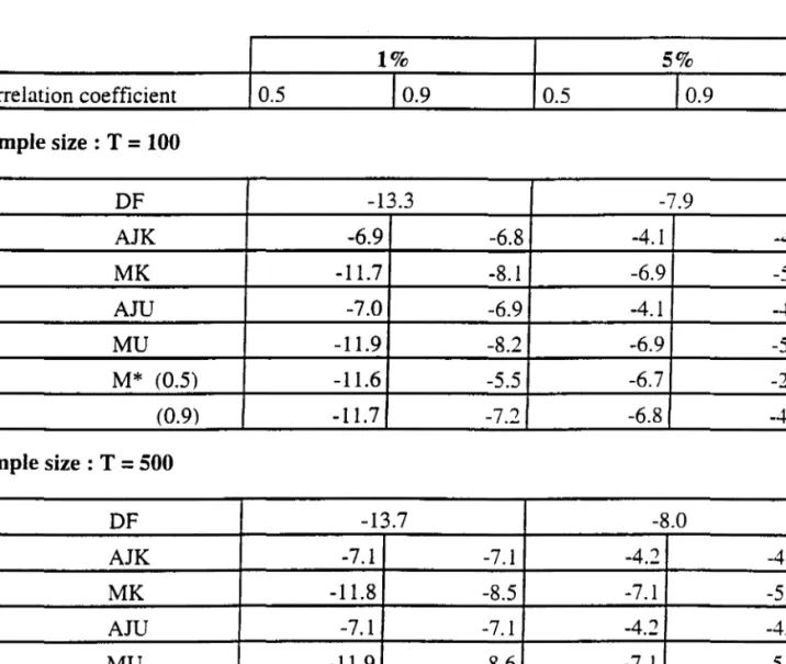
TabIe 1 gives, for p=2, the criticaI 1 % and 5% vaIues for the statistic T(

á)

-1), in the cases T=lOO and T=500. The figures were generated by 5000 replications, with the residual process having unit variances and correIation coefficients of ±O.5 and ±0.9. A simpIe symmetry argument - supported by the formulae in Section 2 - makes it necessary to show onIy the results for positive correIations. To give an idea of the accuracy of the Monte Carlo simuIations, DF vaIues were aIso generated and are displayed in the first row of each sample size.

Table 1. : criticai 1 % and 5 % values for T

(â

_{i -} 1).

1% 5% correlation coefficient 0.5 10.9 0.5 10.9 Sample size : T = 100 DF -13.3 -7.9 AJK -6.9 -6.8 -4.1 MK -11.7 -8.1 -6.9 AJU -7.0 -6.9 -4.1 MU -11.9 -8.2 -6.9 M* (0.5) -11.6 -5.5 -6.7 (0.9) -11.7 -7.2 -6.8 Sample size : T = 500 DF -13.7 -8.0 AJK -7.1 -7.1 -4.2 MK -11.8 -8.5 -7.1 AJU -7.1 -7.1 -4.2 MU -11.9 -8.6 -7.1 M* (0.5) -11.1 -4.2 -6.3 (0.9) -11.7 -5.2 -6.5

For alI the four tests. the increase from 100 to 500 observations does not change much the criticaI values. AIso, as suggested by the asymptotic results, there

is

practically no variation whether the disturbances correlation

is

known or consistently -4.1 -5.3 -4.1 -5.3 -2.8 -4.0 -4.3 -5.5 -4.4 -5.6 -2.4 -3.0

estimated. On the other hand, though the magnitude of the correlation itself does not affect much the AJ abscissae, it has an important impact on the non-constrained M version. This, combined with the fact that AJ's values are always stricter, simply reflects what has been mentioned in the previous section. By using the very hypothesis in the estimation procedure, the constrained AJ tests surely produce stricter criticaI values under the null. In the unconstrained M versions, the higher the residuaIs correlation the more one gains with the multivariate procedure and the closer one moves to the constrained values.

The table is completed with two additional rows, denoted by M*, for each sample size. These rows give the criticaI values corresponding to the case where the second root is stationary, under known variances and covariances. Though the asymptotic distribution is here independent of the particular value of the stationary coefficient, two values (0.5 and 0.9) were tried to check the behaviour in finite samples. Again, the magnitude of the correlation plays a central role. This effect is reasonably less pronounced at T=500.

It is also worth noticing that, for all tests except M*, the criticaI values increase slíghtly wíth the sample size because of the non-stationaríty of the simulated processes. The opposite is true with M* sínce the stationary component attenuates the asymptotic impact (see the end of Section 2).

3.2. Power.

Víolations of the null can take place in many ways. To check the performance of the different tests, the null (2.2) was violated by alternatives with one statíonary coefficient of respectively 0.50, 0.90 and 0.97, supposing, again, residuaIs correlations of 0.5 and 0.9. For each case, 1000 runs were made.

Table 2 shows the percentage of correct diagnoses for the constrained (AJU) and unconstrained (MU) tests, wíth the values obtained with the univariate DF - test shown to ease the comparison.

Now, the correlation matters significantly for the constrained test as it acts in the same direction as the <X2 values. Indeed, with a low <X2' the resulting estimate is a compromise between both values and the percentage of incorrect diagnoses is high.

•

However, it is less bad if the correlation is higher, as fuller use of the estimation technique is made.

Table 2 : Percentages of correct diagnoses for aI .

correlation DF AJU MU aI = 1 ; a2 = 0.50 0.50 94.7 69.4 95.5 0.90 95.2 85.7 99.0 aI = 1 ; a2 = 0.90 0.50 95.3 77.3 95.3 0.90 94.6 93.1 97.3 aI = 1 ; a2 = 0.97 0.50 94.7 86.4 95.1 0.90 94.0 97.3 94.8

On the other hand, the unconstrained MU test performs rather well, with a slight tendency to overaccept. In any case, it is much more robust than the AJU's.

The situation gets worse when we tum to the stationary coefficient estimation. As Table 3 shows, the AJU test, as expected, performs very badly3. The MU version performs very well until 0.90, and still remains superior to the other two at the already misleading value of 0.97.

Table 3 : Percentage of correct diagnoses for a2

correlation DF AJU MU aI = 1 ; a2 = 0.50 0.50 100.0 30.7 100.0 0.90 100.0 14.3 100.0 aI = 1 ; a2 = 0.90 0.50 77.7 22.7 88.6 0.90 76.6 6.9 99.6 aI = 1 ; a2 =0.97 0.50 15.6 13.6 22.4 0.90 16.2 2.7 26.7

3 ActualIy, the AJU column equals, but for a round-off error, 100 minus the corresponding column value in Table 2.

Summing up, there is an evident advantage in performing the multivariate tests. Moreover, contrary to the basic intuition, the unconstrained version should be used in the first step of the procedure.

IV. CONCLUSIONS.

Exploration of the multivariate structure of the disturbances of related series produces fruitful results in unit root testing. Actually, the unconstrained estimation proposed in this paper seems to represent an adequate compromise between the classical Dickey-Fuller approach and the multivariate constrained methodology suggested by Abuaf and Jorion. From the forme r, it keeps the flexibility of individually testing the coefficients while, as in the latter, it exploits the correlations between the senes.

This paper has provided some preliminary evidence of the possible advantages of the proposition and produced some estimates of a few criticaI values. Further work is needed in order to generate a complete set of tables for practical use. Moreover, a deeper power study, investigating the behaviour under problematic error structures like moving-averages is needed to fully certify the proposal.

Appendix: Proof of the asymptotic results.

Proof of (2.8)

If ai = a2 = a, model (2.3) can be rewritten as:

{

Xt =

a

Xt-I

+

U_t

(i\.I) .

Yt =

a

Yt-I

+

Vt

Xo = Yo = O.

The inverse of the matrix

n

will be denoted:

If a in (i\.I) is estimated by a SURE procedure under the equality constraint, given observations {Xt'Yth=I ....• T' the formula for the estimator will be:

I I 12(~ ~ ) 22

(_{n.._} A"') _{a - I} ~ _ a LXt-IX t +0' _{I "} ~Xt-IYt ₁₂

+

~Yt-IXt _"'2 +0' LYt-IYt _.,

~ ~x- +20' ~x Y +0'- ~Y-v ~ t-I ~ t-I t-I ~ t-I

Given model (i\.l), under the null one gets :

,.,

Dividing the numerator and denominator in the RHS of (i\.3) by (T - 1)-, and taking into account the links between the eIements of

n

and O-I standard functional centrallimit results for I(1) processes lead to:

(1\.4)

T(ci-I)=>

I I

0'110'22 JW u (s)dW u (s) - 0'12 ~alla22 [W u (l)W y(l) - P12]

+

0'110'22

f

W y (s)dW y(s)

(1' T)

_{l m - -} O O

tiooT-l . I 2 I I 2

0'1 la22JW u(s)ds - 2a12-Jal 10'22 JW u(s)W y(s)ds

+

0'1 la22JW y(s)ds

I •

where {WU(S)}SE(O,I] and {Wy(S)}SE(O,I] are standard brownian motions associated respective1y to

{,j~'J

et

{~}.

After simplification, (AA) leads to the limit distribution in (2.8).

Proof of (2.11)

The unconstrained estimator of the autoregressive coefficient aI in (2.3) will be:

(A.6)

Under the null, this willlead to:

(A.7)

After dividing both members ofthe RHS by (T-1)4, use ofthe asymptotic theorems and of the relations between the elements of

n

et

n-

I gives the result.

Proof of (2.12)

The stationary hypothesis implies that :

. 1 2 1

phm - LYt-1 = (j2

':"-

.

f

Moreover, as -1-IXt_I.Yt_1 weakly converges to a non-degenerate variable,

T-1

1 2 IXt-I.Yt-1 converges in probability to zero. The result follows then from

(T -1)

N.Cham. P/EPGE SPE F961m

Autor: Flôres Junior, Renato Galvão. Título: Multivariate unit root tests.

1111111111111111111111111111111111111111

~;:a;

73

FGV - BMHS N" Pat.:F3306/98

000089373

I