Revista do Instituto de Geociências - USP Geol. USP, Sér. cient., São Paulo, v. 13, n. 1, p. 3-24, Março 2013
Abstract
The quantification of flow components is important for water resource management. The base, interflow, and runoff flows of nested basins of the Paracatu River (SF-7) were estimated with recursive signal filters in this study. At first, stationary analysis and multivariate gap filling were applied to the flow data. A methodology is presented, proposing filter calibration with the runoff influence and inflection of the recession curve for dry season. Filters are improved with a logic constraint that limits water flow overestimation within algorithm iteration. The results were coherent with previous studies and with hydrogeological and climatological maps.
Keywords: Hydrogeology; Hydrology; Recursive signal filters; Base flow; Aquifers; Water resource management.
Resumo
A quantificação dos componentes de vazão é importante para a gestão de recursos hídricos. Empregaram-se, neste estudo, filtros recursivos de sinais para delimitação dos fluxos de base, interfluxo e rápido de sub-bacias aninhadas na Bacia do Rio Paracatu (SF-7). Preliminarmente, os dados de vazão tiveram sua consistência avaliada por meio de análises de estaciona-lidade e preenchimento multivariado das lacunas de dados. Apresenta-se uma metodologia em que os filtros são calibrados pela influência do escoamento superficial e pela inflexão na curva de recessão do período sazonal de seca. Os filtros foram aprimorados por uma restrição lógica, que limita a sobre-estimação da vazão à cada iteração do algoritmo. Os resultados foram condizentes com estudos prévios e com mapeamentos hidrogeológicos e climatológicos.
Palavras-chave: Hidrogeologia; Hidrologia; Filtros recursivos de sinais; Fluxo de base; Aquíferos; Gestão de recursos hídricos.
Estimation of flow components by recursive filters: case study of
Paracatu River Basin (SF-7), Brazil
Quantificação dos componentes de vazão por meio de filtros recursivos: estudo de caso da
Bacia do Rio Paracatu (SF-7), Brasil
Vitor Vieira Vasconcelos1,2, Paulo Pereira Martins Junior2,3, Renato Moreira Hadad4
1Assembleia Legislativa de Minas Gerais, Rua Rodrigues Caldas, 30, Santo Agostinho, CEP 30190-921, Belo Horizonte, MG, BR ([email protected])
2Universidade Federal de Ouro Preto - UFOP, Campus Morro do Cruzeiro, Ouro Preto, MG, BR
3Setor de Técnicas de Análise Ambiental, Diretoria de Desenvolvimento Tecnológico, Fundação Centro Tecnológico de Minas Gerais, Belo Horizonte, MG, BR ([email protected])
4Departamento de Geografia, Instituto de Ciências Humanas, Pontifícia Universidade Católica de Minas Gerais, Belo Horizonte, MG, BR ([email protected])
Received 03 October 2011; accepted 06 September 2012
INTRODUCTION
Hydrograph separation between superficial runoff components and the base flow is important for water resource management, especially when referring to dry and flood conditions (Tularam and Ilahee, 2008); reservoir navigation and maintenance (McMahon and Mein, 1986); ecological flow, salinity and al-gae management (Santhi et al., 2008); and nutrient and con-taminant outflows into water body (Reay et al.,1992; Dolezal and Kvítek, 2004; Schilling and Zhang, 2004). The compo-nents of hydrograph separation can also serve as input data for more complex models, such as those for water budget and hydrological forecasting (Corzo and Solomatine, 2007). By analyzing the groundwater contribution to each sub-basin flow of water courses, it is possible to adequately define how each area effectively contributes for recharging and discharg-ing of the aquifers.
Specific mapping of the groundwater discharge by sepa-ration of its hydrograph components, in nested basins, can be a useful diagnostic tool for articulating issues involv-ing environmental policies and water resources, with the objective of developing a sustainable management frame-work. This applies to the geo-environmental management context in which government intends to gradually imple-ment manageimple-ment policies, such as water tax and payimple-ment for environmental services. Mapping makes it possible to recognize the relative importance of each basin sub-region regarding the underground water supplied to the rivers. With this information, water and soil conservation man-agements can be valued, mainly in the most critical areas. Thus, one of the adapted policies could be that whoever best contributes to the recharge maintenance of the aquifer would pay less for water usage, or maybe, as a counterpart, would be paid for the environmental service provided. Since most water resource conflicts occur during dry seasons, when river flow is sustained mainly by groundwater dis-charge, the base flow (and its respective mapping) quantifies the most critical characteristics to be considered. In addi-tion, quick flow mapping could indicate areas that are inter-esting for the implementation of flow retention and regular-ization techniques, which involve water containment during the rainy season and its liberation during the dry season.
As proposed by Johnson et al. (1999), Dillon (2005) and Martins Junior (2006), the final objective of a poli-cy that integrates orderly sustainable land and water use would be to hydrogeologically and economically quantify the feasibility of increasing infiltration in areas of great-er recharge potential during the rainy season, in ordgreat-er to guarantee an adequate minimum flow during the dry sea-son and improve water quality.With future demanding more refined environmental management, the standards established by distinct entities (federal, state and munici-pal, together with those directly involved with watersheds)
could provide the needed degrees of protection or conser-vation, which would be gradually defined as hydrogeolog-ical knowledge increases. Therefore, at a given site, sci-entifically reliable intervention could be practiced for the sustainable usage of its natural resources.
Gap filling in hydrological data series
The stationary evaluation of hydrological data in time se-ries is justified by the fact that it is assumed to be necessary for hydrological and hydrogeological statistical modeling (Tucci, 2009; Souza et al., 2009), including its use to estimate input data for gaps in the flow data series. Noteworthy is the methodological attitude proposed by Müller et al. (1998), who claims that stationary study of hydrological time series should be employed as a tool to aggregate information and for comparative analyses, which would be more than simply hypothesis rejection testing.
As a preparatory step for filling in the flow gaps from the stream gauges, the Brazilian National Water Agency (Souza et al., 2009) recommends the grouping support ap-proach of gauging stations. This methodology consists of selecting data from stations that are topologically closer downstream and upstream of the gauging station from which the gaps are being filled. It is also feasible to include data from stations in nearby basins, providing these basins have homogeneously physiographic characteristics. The stations whose data present the greatest correlating coef-ficients are used for filling in the gaps. Rodriguez (2004), Novaes (2005), Moreira (2006), Latuf (2007) and Souza (2009) used the gauging station support approach for hydrological studies at the Paracatu River Basin.
Schafer and Graham (2002), Allison (2002) and Enders (2010) classified expectation maximization (EM) (Hartley, 1958; Dempster, Laird, Rubin, 1977) and mul-tiple imputation(MI) as the most robust methods available for gap analysis in statistical databases. The algorithms from both methods are present in the Statistical Package for the Social Sciences (SPSS) software model — missing values. Presti et al. (2010) indicate that using multivariate techniques (such as EM and MI) increase the statistical reliability of hy-drological data gap filling. Thus, it is possible to work with greater gap percentages or shorter time series. Furthermore, since accurate flow estimates of the hydrogeological basin re-quire daily runoff data, extra statistical care must be provid-ed to ensure that data validation is more reliable, rather than when working with only a series of monthly measurements.
heterogeneity of rainfall occurrence registered in nearby gauging stations and in the station requiring gap fillings.
Amisigo and Vand de Giesen (2005), in applied studies, demonstrated that the EM technique provides more precise estimations of flow data gaps, when compared to the classi-cal regression ones. Enders (2010) mathematiclassi-cally showed how EM estimation is more robust in relation to data dis-tribution presuppositions, when compared to conventional regression techniques. In addition, EM input presents an advantage over multivariate regression by maximizing its statistical power through information obtained from the dis-tribution curve of incomplete cases, and by estimating the original time series variance level (Enders, 2010).
Meanwhile, MI adds a random residual to the selected multiple regressions (analogically to a stochastic multiple regression), so that the results maintain the original vari-ance of the observations as a whole. However, even though this random residual keeps the original variance, it distances the input value “at the same measurement” in relation to its maximum probability value, thus reducing data estimation reliability. Cano and Andreu (2010) alerted that in series with significant time correlation such as that with hydro-logical data, the sum of random residual by the conventional MI algorithms could lead to results that are less compatible with the natural behavior of real data.
Also, Enders (2010) stated that the methodology op-tions of MI algorithms are not as mature, consolidated, and tested as those of EM. On the other hand, an existing broad study by Amisigo and Vand de Giesen (2005) about EM, applied to gap filling in hydrologic data, brought more se-curity for using such methodology.
Presti et al. (2010) suggested that in unimodal oscillating climates (contrast between dry and rainy seasons, as in the case of the Paracatu River Basin), the gap filling should be applied separately for two periods of the year: rainy and drought. Thus, the distinct water flow dynamics at each of these two seasons will be captured with more assurance in their correlation. In the dry season, it is expected that the coefficient of the recession curve in logarithmic scale, in each basin, will be one of the de-fining characteristics of the correlation for lag filling. The rainy period, in turn, would present a major influence from the flux characteristics referring to the separation between superficial, subsurface, and groundwater flows.
Base flow estimation
Field and direct inference methods are amongst the most widely used for base flow inference. The field methods include direct monitoring of the aquifer level (by wells and/or piezometers), correlations parting from water temperature obtained by direct measurement or tracers, and infiltration monitoring by lysimeters. However, the employment of these techniques for large basins involves
exorbitant costs due to the extensive sampling network required and creates uncertainty because of the spatial heterogeneity of hydrogeological processes.
Regarding techniques that try to specify the base flow by indirect inference, the most common are: water budget, hydrograph component separation, calculation of the flow recession (equation from Rorabaugh, 1964), and system-atic comparison between rainfall events for hydrological pulses analysis (Su, 1995).
Nevertheless, because the hydrograph separation methods focus only on the base flow of watercourses, they do not incorporate the quantitative loss concerning river evapotranspiration and deep percolation that crosses be-neath the gauging station (Risser et al., 2005). These two factors are important for the recharge analysis of the aqui-fers since they interfere in the water budget of the basin.
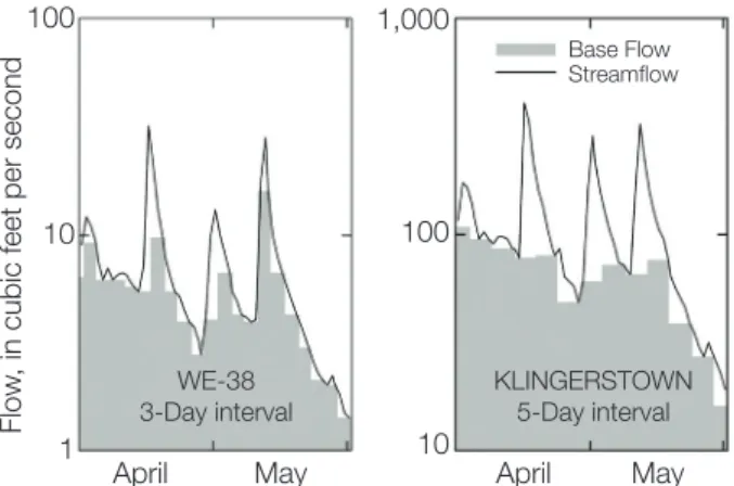
Base flow separation by means of computational calcu-lations eliminates the imprecision and inherent subjectiv-ity of the traditional graphic methods as those proposed by Barnes (1939). However, Risser et al. (2005) noticed that conventional hydrograph separation by numerical meth-ods (PART, local minimums fixed intervals, fluctuating in-tervals) might create difficulties for comparing base flow estimates of different-sized basins (including the nested ones). An increase in basin area implies: greater runoff time, flood lessening, bed friction on the flow, partially simultaneous flow contributions from tributaries, and re-gional hydrogoeological flow, among other factors, which can rarely be automatically calibrated by the available al-gorithms. Figure 1 highlights how these methods can gen-erate distortions in base flow separation.
100
10
1
Flow
, in cubic feet per second WE-38
3-Day interval April May 1,000 100 10 KLINGERSTOWN 5-Day interval April May Base Flow Streamflow
The numerical methods for recharge calculations through recession curve analysis, theoretically, are not affected by this limitation. As such, instead of starting with the recognition of the inflection point (like hydrograph separation methods), the methods for analyzing recession begin by identifying flow peaks, after which the flow recession behavior is calculated (Rutledge, 1993, 1998, 2000). In order to analyze flow reces-sion, it is necessary to calibrate the critical time (tc), that is, the period to cease the influence of runoff. To achieve such thing, Rutledge (1993) and Welderufael and Woyessa (2010) refer to the empirical formula made by Lynsley et al.(1975):
N = 0.827* A0.2 (1)
where:
N: time (in days) after hydrographic peaking to stop the participation of runoff; and
A: is the area of the basin, in km2.
Notwithstanding, this formula presumes that the rain-fall event covered the entire basin — a criterion that makes the equation less reliable with the basin area increase.
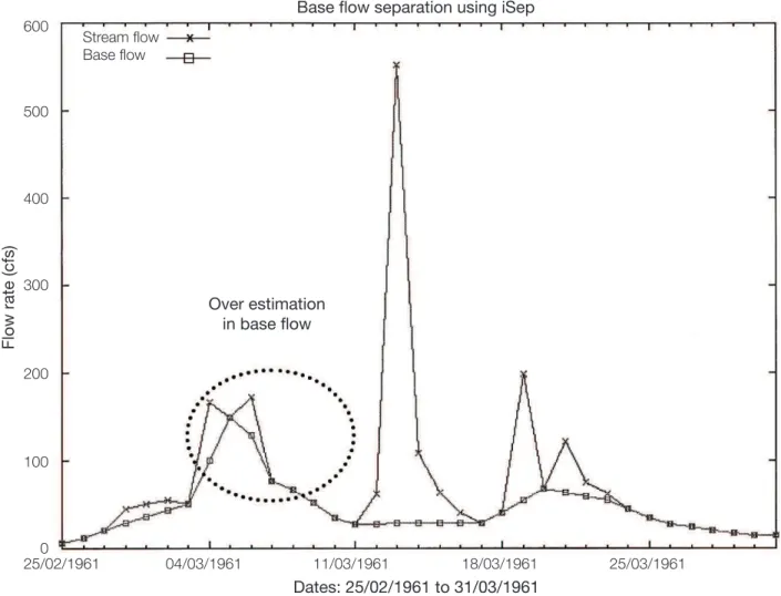
For greater reliability of the recession curve analysis, it is necessary to identify relatively long and continuous re-cession periods (without intercurrent flow peaks) (Halford and Mayer, 2000). Care must be taken so that abnormally low flow periods are not presented as part of the standard behavior of the water system (Rutledge, 2003). Halford and Mayer (2000) and Larocque et al. (2010) observed that the manual and automatic hydrograph separation methods, when applied based on analysis of recession at closely spaced peaks related to intercurrent rain, could lose their reference criteria and as such diminish the reliability of the component separation process. Furthermore, it would tend to overestimate the base flow value by considering a reces-sion flux, which is still under the effects of superficial and subsurface runoff from recent rainfall events (Figure 2).
600
500
Stream flow Base flow
Base flow separation using iSep
Flow rate (cfs)
Over estimation in base flow
400
300
200
100
0
Dates: 25/02/1961 to 31/03/1961
25/02/1961 04/03/1961 11/03/1961 18/03/1961 25/03/1961
In order to incorporate the advantages of recession anal-ysis into criteria for hydrograph separation without distort-ing them by the use of temporal interval variables, an alter-native would be to use digital recursive filters. With their use, it is presumed that the low-frequency waves of the hydrograph inform the base flow, while the high ones re-late to the runoff (Lim et al., 2005). The sum of both waves corresponds to the total flow of the hydrograph.
Peters and Van Lanen (2005) and Brodie and Hostetler (2005) state that the inherent disadvantage of the recursive filters is that they rely only on the hydrograph form, with-out a sustainable base of physical parameters. To over-come this problem, Ghanbarpour, Teimouri and Gholami (2008), Asmeron (2008), Tularam and Ilahee (2008) and Lim et al. (2007, 2010) proposed the possibility of cali-brating the recursive filter parameters, based on the reces-sion curve analysis of the hydrograph.
OBJECTIVES
This article had as a general objective to present a study about flow components of the sub-basins of Paracatu River, furnishing data to improve the management of its water resources. To achieve this, the following specific tasks were undertaken:
• stationary analysis of the flow average and variance for the gauging stations in Paracatu River Basin;
• discharge gap filling with the use of the multivariate techniques EM and MI;
• filter calibrating with double parameters, i.e., runoff in-fluence and recession curve inflection;
• incorporation of a logical restrictor to estimate the base flow of recursive filters, impeding an overestimation of
the base flow participation in the total discharge calcu-lated by each iteration of the algorithm;
• spatial analysis of the relationship between base flow estimation and its geographical data regarding climate and hydrology.
It is worthnoting that preexisting studies using recur-sive filters have yet to focalize on the comparison of basins with diverse sizes. This article, by encompassing the con-catenation between Paracatu Basin and its nested basins through readings from internal gauging stations, presents unique scientific data.
METHODOLOGY
Paracatu River Basin characterization
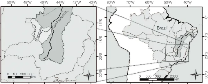
The Paracatu River Basin is almost totally located in Northwestern Minas Gerais, in Brazil with a small up-stream area in the State of Goiás and Federal District (Figure 3). The basin has an extension of 45,154 km2, and it is the largest among all the affluents that flow directly into the São Francisco River.
The Paracatu River Basin has a megathermic rainy climate of the Aw type (IGAM, 2006). It is a typically rainy tropical with high temperatures and oscillating un-imodal precipitation concentrated in the months from October to April, when it rains an average of 93% of the total annual rainfall (Mulholland, 2009). Figure 4 shows the rainfall distribution. From the basin’s climatic charac-terization by Ruralminas (1996), it becomes evident that there is a spatial correlation between the precipitation data and other climatic variables, such as temperature,
50ºW
Brazil
48ºW 46ºW 44ºW 42ºW 40ºW 80ºW 70ºW 60ºW 50ºW 40ºW
16ºS
18ºS
20ºS
22ºS
0º
10ºS
20ºS
30ºS
0 100 200 300
km 0 500 1000 2000
km
São Francisco
Paracatu
solar radiation, humidity, evapotranspiration, cloudiness, water stress, and storm frequency.
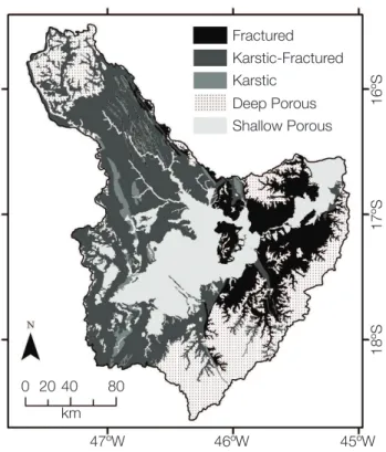
The Paracatu River Basis stratigraphy presents dis-tinct rock systems that support aquifers (Figure 5). By means of the graphic method proposed by Barnes (1939), the Minas Gerais Technological Center Foundation (CETEC, 1981) estimated that, for the Paracatu River Basin, at different points, from 32 to 48% of the watercourse flow is maintained by under-ground aquifers. This contribution increases as the wa-tercourse passes through recharge areas of cretaceous sandstones and tertiary-quaternary sedimentary cover, and therefore they were characterized as favorable re-charge areas. In addition, these calculations considered that the infiltration and contribution from the fractured and Karst formations of Bambuí aquifer would be very low or virtually nonexistent when compared with the aforementioned granular aquifers. Ramos and Paixão (2004) also highlighted the importance of porous sedi-mentary aquifers for the perpetuation of rivers feeding São Francisco River Basin.
Areado and Urucuia Formations (Cretaceous) are characterized by free aquifers that furnish a significant amount of water through hillside sources (CETEC, 1981) and possibly through direct effluence along streams. They are formed by thick sandstone (up to 140 m) and lie di-rectly on an impermeable substrate of the Bambuí group (Eo-Cambrian) (CETEC, 1981). However, the underly-ing mesofractures identified in the Bambuí Formation may increase the complexity of these aquifers through the combination of fractured and granular aquifers (Martins Junior, 2006). Mata da Corda Formation, with up to 100 m
thickness, also has a porous aquifer overlying the Aerado Formation (RURALMINAS, 1996).
Morphologically, porous aquifers of the older tertiary-quaternary cover lie underneath part of the São Francisco Residual Plateaus, forming tabular surfaces with a height of more than 900 m (Andrade, 2007). In the Paracatu River Basin, the tabular surfaces are scarcely reworked and have almost no drainage. These characteristics are due to a thick sedimentary layer with high infiltration poten-tial (CETEC, 1981). The main discharge areas are located at the foothills of the elevations, along the flank or edges of the plateaus, where there is contact between the aquifer and an impermeable substrate. These aquifers have an av-erage thickness of 10 m and can exceptionally attain 30 m (RURALMINAS, 1996), with a registered record of up to 80 m (Mourão, 2001).
The more recent tertiary-quaternary sedimented aquifers are located in the river plains of Rio Paracatu River Basin, lying atop the Bambuí Group pelites with low permeability, whereupon there is frequent exudation in the contact area of two lithologies (CETEC, 1981; Mourão, 2001). Due to predominant geomorphology of the plane surfaces of this aquifer system (Andrade, 2007), CETEC (1981) hypoth-esize that local and regional base flows exist where there are hydraulic connections between aquifers and rivers — in this way, the aquifers function as flow regulators of such
48ºW
15ºS
47ºW 46ºW 45ºW
0
16ºS
17ºS
18ºS
km 20 40 80
Figure 4. Annual average rainfall for Paracatu River Basin (in mm), based on data from Nunes and Nascimento (2004).
Fractured
16ºS
Karstic-Fractured Karstic
Deep Porous Shallow Porous
17ºS
18ºS
47ºW 46ºW 45ºW
0 20 40 80 km
watercourses. The water storage potential is less than in the other porous aquifers of the basin, due to the narrowness — an average of 5 m (RURALMINAS, 1996).
Fractured aquifers occur in the Bambuí and Canastra Groups, as well as in the Paracatu, Vazante, and Paranoá Formations. Their storage capacity depends on their frac-ture extension, continuity and interconnections, together with their opening and interior void volume. In compar-ison with granular aquifers, the possibility of direct rain infiltration in these fractured rock reservoirs is small be-cause the fractures are narrow (Mourão, 2001). The re-charge happens by vertical infiltration from an upper shal-low aquifer or by deeper infiltration from the cretaceous and tertiary-quaternary sedimentary layer covers, as well as by points where both fracture and drainage coincides, that is, through watercourses controlled by fracture direc-tion (RURALMINAS, 1996).
The Karstic aquifers of the Paracatu Basin predomi-nantly correspond to geomorphological areas consisting of ridges and steep slopes (Andrade, 2007). Since they are distributed along the deformation zone of the Unaí Ridge and were submitted to strong tectonism (transcurrent and thrust faulting, as well as folding structures), it is assumed that there is a high degree of fracturing. Furthermore, the presence of sinkholes, caves and sinks indicates endokarst development by dissolution. It can also be presumed that these aquifers enable a significant hydrogeological flow. In evolved Karstic forms, the expressive flow from their inherent ducts produces aquifers with accentuated reces-sion coefficients because as the water leaves them quickly, they provide little water for the springs during the apex of the dry season.
The quaternary alluvial deposits are usually found along the drainage system, in flood plains and in terraces. They are active zones for water exchange, for receiving recharge from the rivers during rainy periods, and for dis-charging it during dry periods (Mourão, 2001).
In the transition areas between the residual plateaus and the São Francisco depression in Paracatu Basin, the domi-nant reworked geomorphological features of the hills and slopes are regions where the hydrological role of transient flow occurs. This is because their localization is between the aquifer systems and due to the fact that the greater inclina-tion disfavors rain infiltrainclina-tion in these areas. Nevertheless, it is good to remember that all surfaces with a weathered cover contribute in part to groundwater recharging.
Component flow estimation of the basins with gauging stations
Data source for the analyses performed for this article is the record of gauging stations flow available on the Internet for all regions in Brazil, supplied by the hydrological
Information system (Hidroweb) of the Brazilian National Water Agency (ANA, 2008).
Rodriguez (2004), Novaes (2005), Moreira (2006) and Souza (2009) opted for the period between 1970 and 2000 (30 years), and selected and evaluated the use of 19 to 21 gauging stations at the Paracatu River Basin as consistent. However, the analysis of the operation history of these stations shows that a greater part of them became opera-tive between 1975 and 1976. Consequently, by choosing a main set of stations from 1976 to 2000, it was possi-ble to mount a basic block of 23 stations, minimizing the gap filling and series extension uncertainties. July of 2001 was the period’s limit due to the beginning of interventions for the construction of the Queimado Hydroelectric Power Plant, at the sub-basin of Preto River after which the hy-drological behavior of the area would influence data.
Two gauging stations were also selected with periods in-ferior to that of the main block: 426450000 (1974 – 1984) and 42350000 (1973 – 1981). These stations received differ-ential treatment that will be further elaborated in this article.
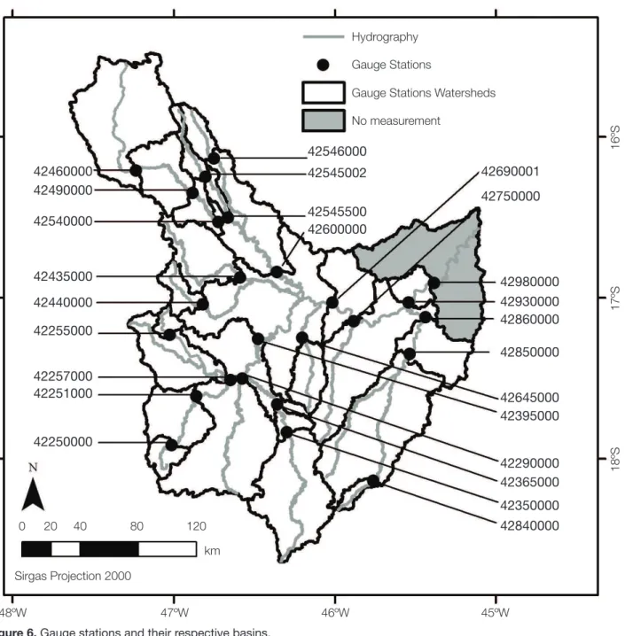
The location of the gauging stations used in this article with their respective nested basins is shown in Figure 6. The basin drainage delimitations related to gauging sta-tions were elaborated on the basis of a hydrologically consistent digital elevation model. It was based on the topographic treatment of Shuttle Radar Topography Mission (SRTM) — data and on the IBGE hydrogra-phy (1:100.000), reconditioned with the Hydrotools for ArcGis 10 extension and with pre-processing algorithms of the Saga 2.0.8 program in order to obtain altimetric consistency regarding the runoff from the slopes, the len-tic water bodies, and the drainage network.
Stationary analysis was performed by means of tests combined with Fisher’s equality of variance and Student’s equality of averages, as recommended by Tucci (2002) and by the Brazilian National Water Agency (Souza et al., 2009). About the gauging station data, tests for average, minimum and maximum stationarity at 1 and 5% level of significance were performed to analyze the average and monthly variations, with successive tests of minimum five-year groupings in continuous combinations for all the possibilities of grouping in series, for the hydro-logical period from 1976 to 2000. Analogously, station-arity tests were also performed for the period of 1957 to 2000 at the oldest four gauging stations of the Basin. The tests were carried out on SisCAH 1.0 program, which is available without any costs at the Brazilian National Water Agency website.
The preliminary grouping of support stations consid-ered: areas of homogeneous water systems proposed by Euclydes (2004); drainage pattern areas by Martins Junior (2009); spatial variations of the cartographic bases (geol-ogy, geomorphol(geol-ogy, soil, slope, and height) by Martins Junior (2006); topological connection of the drainage net-work; stationarity tests; and correlation coefficient among the discharges time series. Also taken into account were the areas with a homogeneous annual rainfall rate, which would also be spatially correlated with the other cli-matic parameters of the basin.
Filling in the gaps with EM and IM involved using data from before 1976, when available, to amplify the com-parison possibility for the statistical distribution of the dai-ly discharge at the referenced gauging station with those of the selected support gauging stations. For the gauging stations that were not affected by the construction of the Queimada Hydroelectric Plant, discharge data from 2001 on were also used.
From the point of view of existing conflicts con-cerning water usage in the Paracatu Basin for irrigation (Pruski et al., 2007), it can be questioned if this water
Hydrography
42460000
16ºS
Gauge Stations
Gauge Stations Watersheds
No measurement
48ºW 0
42490000
17ºS
18ºS
47ºW 46ºW 45ºW
20 40 80 120
km
Sirgas Projection 2000
42540000
42546000
42545002
42545500 42600000
42690001
42750000
42435000
42440000
42255000
42257000 42251000
42250000
42980000 42930000 42860000
42850000
42645000 42395000
42290000 42365000
42350000 42840000
consumption does not influence the consistency of the discharge analysis for the gauging stations. However, re-search performed by Rodriguez (2008) demonstrated that this water consumption for irrigation presented less than 10% effect on the minimum (Q7,10) and permanent (Q95) discharges of Paracatu Basin. Vasconcelos (2010), when analyzing the study performed by Rodriguez (2008), re-garding a comparison of the gauging station locations in relation to the irrigation areas, pointed that the existing gauging stations are located in the main river beds. These are far downstream from the tributaries used for irrigation, so that the readings from the gauging station already incor-porate this usage, together with the discharge from larger tributaries. Thus, the impact of local irrigation is masked and is difficult to measure, although it reduces the bias in regional hydrological analyses.
Hydrograph separation
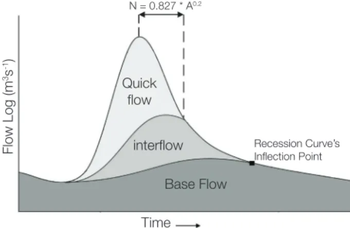
Nathan and McMahon (1990) and Albuquerque (2009) stated that the available hydrograph separation methods do not present a criterion that permits reliable delimitation of the subsurface flow, which is found in the hydrograph region between the base flow and surface discharge. To improve this situation, this study proposed combining the results of two recursive filters used as follows: calibrated in reference to the recession exponential curve for the dry season, more accurately corresponding to the base flow; and calibrated in reference to the influential point of runoff discharge using the Lynsley et al. (1975) empirical formu-la, which corresponds to the sum of the base with the sub-surface flow. Both parameters were calibrated so that they may attend the best possible approximation to the conven-tional graphic projection models for the recession curve (Barnes, 1939), and the undulatory overlying of the hy-drological response units (Su, 1995). In order to calibrate the runoff discharge point of influence, isolated rain peaks, without data gaps, were chosen to be in accordance with the empirical formula referred by Lynsley et al. (1975).
The concept model for this type of hydrograph is presented in Figure 7.
Another problem found regarding the recursive filters is the mathematical possibility that the base flow estima-tion is superior to the total discharge value for the river at some hydrograph periods. To overcome this problem, Gregor (2010) proposed that a cut should be done in the overestimated discharge at the end of the filter algorithm application. Whereas, Chapman (1999) suggested (al-though not explicitly implements) that by using an inter-nal constraint at each algorithmic iteration would provide greater consistency for the one-parameter filter. Adopting the recommendation from Chapman (1999), the follow-ing logic restrictor was implemented: if base flow ≤
to-tal discharge; then, maintain base flow values; if not, base flow equals total discharge.
Table 1 presents the tested filters. The option was for one-parameter filters because they could be more objec-tively calibrated (Chapman, 1999).
Statistical procedures for the spatialization of the hy-drogeological data in nested basins were based on its con-catenation and overlap, in accordance with the methodol-ogy used by Holtschlag (1997). This allowed to elaborate
Quick
flow
Time
Flow Log (m
3s -1)
interflow
Base Flow N = 0.827 * A0.2
Recession Curve’s Inflection Point
Figure 7. Conceptual hydrograph for runoff partitioning.
Table 1. Recursive filters evaluated in this paper.
Recursive Filter Author
qf
(i)=
3α - 1
3 - α qf (i-1)
2 +
3 - α (q(i) - αq(i-1)) Chapman (1991)
q
b (i)=
α
2 - α qb (i-1) + q(i)
1 - α
2 - α Chapman and Maxwell (1996)
qf
(i)= αq f (i-1)
2
+ (q(i) - q(i-1)) 1 + α Lyne and Hollick (1979) – “Bflow”
q
b
(i)= αq(i) + (1 - α) qb (i-1) Tularam and Ilahee (2008) – “EWMA filter”
digital geographic information bases about the flow com-ponents’ contribution towards the discharge at the stretch-es of the nstretch-ested basins of the Paracatu River.
RESULTS AND DISCUSSION
Stationarity
The analyzed gauging stations obtained satisfactory re-sults for stationarity tests regarding the discharge averages and variance at a 5% level of significance. Only station 4286000 was rejected from the stationary variation of min-imum events at a 5% level of significance; and 42365000 was rejected for stationary variance of maximum events at a 5% level of significance. Only one of them had its aver-age stationarity rejected at a 1% level of significance (pass-ing the test at the 5% level). The rest of the rejections re-ferred to variance at a 1% level.
In cases where rejection occurred during the test, their patterns and tendencies were evaluated. An attempt was made to find the breaking point, i.e., the period that best demarcates the stationary difference in accordance with the standard deviation for the constraining peri-ods. Hydrological data analysis shows a period of fre-quent discharge peaks between 1976 and 1985, caus-ing a different impact on each nested basin. Such data was in agreement with discharge studies done by plot-ting of the average monthly hydrographs, performed by Carvalho et al. (2004) for the Paracatu River Basin. This flood interlinking elevated the historical variances of this period, reflecting on stationarity tests for vari-ances at a level of 1%, especially in tests for maximum events. From 1994 until 2000, there is a lessening in the discharge variance of the rivers, provoking rejection in some stationarity tests at a 1% significance level. The gauging stations referring to basins of greater contribu-tion (for example, those on the main bed of the Paracatu River), as expected, presented less interference on vari-ance stationarity since they dampened the flooding ef-fects (for maximum events) and had a possible effect from the regional hydrogeologic flow (for annual aver-ages and minimum events).
In long-term stationarity tests (1957 – 2000), the four gauging stations were approved in the test for the average stationarity of the monthly discharge at a 1% level of sig-nificance. For the stationarity test of variance, the effect of the flood peaks from 1976 to 1985 made three tests (one for monthly minimum, another for monthly average, and the last, for monthly maximum) fail the significance test at the 1% level — although they all passed at the 5% one. Analyses of the two test blocks for stationarity (one from 1957, and the other from 1976) corroborated the statement
that there was a period of lesser parameter variance from 1957 to 1975, as well as from 1993 to 2000.
The good results concerning the stationarity tests for average discharge bring additional reliability for gap fill-ing. Despite rejection of the stationarity hypothesis for variances at a significance level of 1%, it is believed that this break in stationarity does not present a manda-tory impediment to the statistical procedures, consid-ering the results presented in this study. Remember that stationary results for variance served as criteria for the se-lection of support stations to fill in the gaps, generating a grouping of gauging stations under similar conditions. Nonetheless, the tests presented are as a safeguard for fu-ture comparative studies.
Gap filling
As previously discussed, the available state-of-art method-ological options for gap filling (EM and MI) seek a solu-tion that is a compromise between forecast reliability and variance data maintenance. For base discharge separation (hydrogeological flow), the estimative results were ana-lyzed with preference to a greater reliability for forecast-ing from the data, keepforecast-ing in mind that the data filled in will be utilized in mathematical-statistical models that are sensible to temporal correlation patterns.
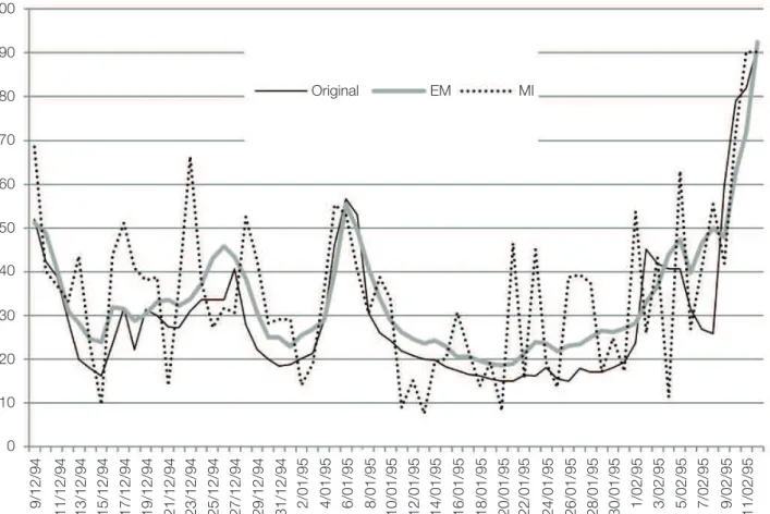
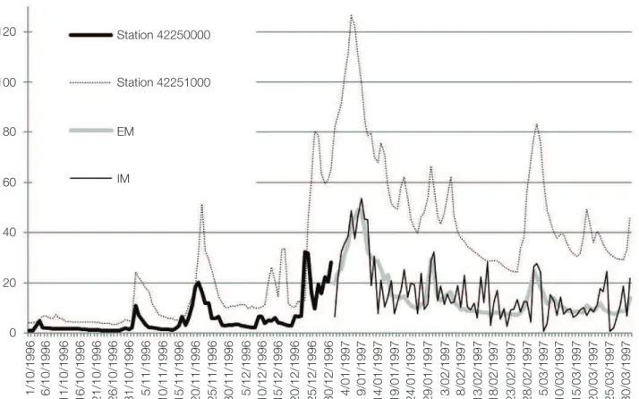
Figures 8 and 9 present comparative examples of the results obtained by estimation using EM and MI. In Figure 8, a gap filling was simulated for an area and original data was used for comparison. For consistency in the MI data, a constraint was used for non-negative data. In both graphics, estimation using EM came closest to the original hydrograph. Figures 8 and 9 show how estima-tion by MI, although following an average tendency, cre-ated an abnormal variance that did not respect the tempo-ral correlation of the hydrograph, corroborating with the theoretical caution proposed by Cano and Andreu (2010). Although the EM line in the graph of Figure 8 is slightly above the original hydrograph, the theoretic base of this method guarantees that in filled in periods as a whole, the average and discharge variance will be the closest possible approximation with original data.
For each gauging station, gap-filling values were con-ferred by exploration through visual analysis of the dis-charge graphs, assuring that the input data was consistent from a hydrological point of view and followed the trends of the support stations.
Flow component delimitation
the estimated base flow did not coincide with the recession curve during the annual dry season (Figure 10).
The filters mentioned by Lyne and Hollick (1979) and by Tularam and Ilahee (2008), after calibration, presented identical visual behaviors. Notwithstanding, the filter mentioned by Lyne and Hollick (1979) was chosen because it is the most widely found in lit-erature (Lim et al., 2005; Combalicer et al., 2008; Asmeron, 2008; Santhi et al.,2008; Albuquerque, 2009; Welderufael and Woyessa, 2010; Biller, 2010), making it easier to compare with other studies.
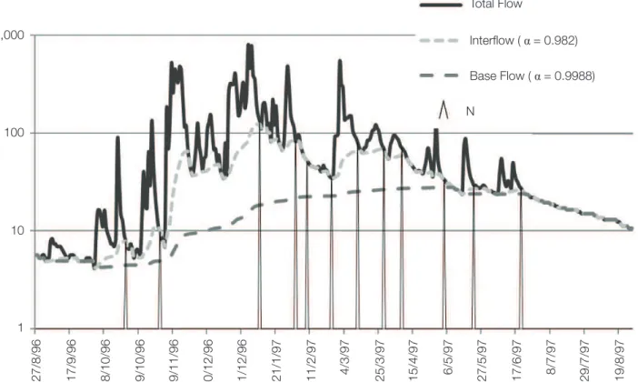
The end of the N period (number of days after the hydrographic peak, when the runoff discharge participa-tion ceased) of Lynsley et al. (1975) empirical equation coincided in a greater part of the hydrographs, with a change in the inclination of the depletion line for the rain peak, corroborating with the reliability of its application. Calibrating the filters with the combined double parame-ters made it possible to clearly separate the interflow wave from the base one (Figure 11).
For the two stations of the isolated series (inferior to the period of the main block), a comparison of the chosen filter with the support stations was done during the same period for which a series of data was available. Following this, the results were compared with those for the com-plete period (1976 – 2001). Average annual discharge value variation, base flow, interflow, and quick flow were used to adjust the respective results for the filter on the isolated series. The average adjustment for the basin data for station 42350000 (1974 – 1984) was -9%, while for 42645000 (1973 – 1981), it was -0.63%.
The results of the calibrated application of the filter at each station and the concatenation of the drainage basins with the data concerning total discharge, quick flow, inter-flow, and base inter-flow, including the specific discharge, are presented in Tables 2 and 3.
For comparison, Table 3 also presents the base flow in-dex (BFI) as a result from hydrograph separation of some of the stations when using Barnes (1939) graphic method, performed by CETEC (1981) and RURALMINAS (1996).
Original EM MI
100
90
80
70
60
50
40
30
20
10
0
9/12/94 11/12/94 13/12/94 15/12/94 17/12/94 19/12/94 21/12/94 23/12/94 25/12/94 27/12/94 29/12/94 31/12/94 2/01/95 4/01/95 6/01/95 8/01/95 10/01/95 12/01/95 14/01/95 16/01/95 18/01/95 20/01/95 22/01/95 24/01/95 26/01/95 28/01/95 30/01/95 1/02/95 3/02/95 5/02/95 7/02/95 9/02/95 11/02/95
The delimitation in RURALMINAS (1996) was done for 1939 to 1989, while the delimitation in CETEC (1981) used only one hydrological year, between 1969 and 1974 for different stations. The BFI, which is equivalent to the division of the base flow by the total discharge, is rela-tively stable at long term in basins, even with the annual discharge variations, which makes feasible the comparison between estimates of different periods (Santhi et al., 2008). Comparison of the estimated indexes from the recursive filters with the estimated base flow by graphic methods demonstrated similar tendencies. Notwithstanding, with data presented in Table 3, it is possible to perceive how the graphic method incorporates in different proportions the interflow in relation to the base flow in each basin, demonstrating the inherent subjectivity of this technique.
As can be seen in Table 2, the average of parame-ters (α, as presented in Table 1) calibrated for the filters
(in the two calibration forms) is superior to 0.925, which is referenced in literature (Nathan and McMahon, 1990; Ghanbarpour, Teimouri, Gholami, 2008). Despite the fact that the hydrological characteristics of Paracatu River Basin have their differences in relation to basins with a temperate climate, this study case generated a hypothesis that the lack of calibration for the influence of runoff dis-charge, together with the inflexion of the recession curve,
could have led the studies with filters, performed in pre-existing ones, to overestimate the base flow discharge val-ues. This is in agreement with Asmeron (2008), who stated that the 0.995 parameter seemed more coherent with the hydrographic curves for the Blue Nile Basin in Ethiopia.
Analysis of the specific discharge maps (Figure 12) col-lated in Tables 2 and 3 shows that the base flow contribution is more significant at the headwaters of the basin because of heavier rainfall, especially in the western portion. This
1,000 100 10 1
Total Flow
1/10/76 1/11/76 1/12/76 1/1/77 1/2/77 1/3/77 1/4/77 1/5/77 1/6/77 1/7/77 1/8/77 1/9/77
Chapman and Maxwell (1996)
filter
Figure 10. Application of the Chapman and Maxwell Filter (1995), with parameter α = 0.925, for the daily discharge
data from Station 42290000, hydrologic year of 1976. Discharge is in logarithmic scale. Notice that the estimated discharge for the base flow during the dry season does not coincide with the total one.
120 Station 42250000
Station 42251000
EM
IM 100
80
60
40
20
0
1/10/1996 6/10/1996 11/10/1996 16/10/1996 21/10/1996 26/10/1996 31/10/1996 5/11/1996 10/11/1996 15/11/1996 20/11/1996 25/11/1996 30/11/1996 5/12/1996 10/12/1996 15/12/1996 20/12/1996 25/12/1996 30/12/1996 4/01/1997 9/01/1997 14/01/1997 19/01/1997 24/01/1997 29/01/1997 3/02/1997 8/02/1997 13/02/1997 18/02/1997 23/02/1997 28/02/1997 5/03/1997 10/03/1997 15/03/1997 20/03/1997 25/03/1997 30/03/1997
configuration also reinforces the recharge role of the pla-teaus that have a porous sedimentary lithology at the ba-sin headwaters. As the stream flows downward towards the lowlands of the central area of Paracatu Basin, the base flow contribution becomes significantly less expressive. This re-sult is also coherent with that related by Tucci (2002), who observed a specific discharge reduction as basin area in-creased in many flow records of rivers in Brazil.
However, it is interesting to note how certain increases in specific total discharge, base, and interflow occur after stations 42930000 (Lower Paracatu), 42490000 (Middle Preto River) and 42350000 (Lower Prata River). It is pos-sible that there are regional underground flows crosscut-ting below the station and surface downstream. This phe-nomenon seems to mainly occur in areas that have shallow lateritic-debris porous aquifers, which receive water from Karstic-fissured aquifers.
As a final comment, it is necessary to recognize that the automatic hydrographic separation methods analyze only form patterns of waves representing discharge pulses, and as such, they do not directly identify the source of dis-charge components. Therefore, the automatic method re-sults are referred to hydrogeological processes only as the base flow, interflow, and quick flow really correspond to underground, subsurface, and runoff flows respectively. In
this context, Kirchner (2003) and Gonzales et al. (2009) studies can be cited for demonstrating that the regional groundwater flow generally responds to rain as quickly as runoff does, due to the piston effect of precipitation in the recharge areas of the basin, while the clay soil of the low-lands retards and dilutes the interflow for a more ample pe-riod. In areas under Karstic influence, there is also a plau-sible hypothesis in that the interflow partially corresponds to the endokarstic duct flow, even after runoff discharge has finished. These hypotheses bring forward a recommen-dation that future studies with tracers could improve the understanding of hydrogeological processes involved.
CONCLUSIONS
The stationary analysis brought greater reliability to the knowledge about the Paracatu River Basin discharge. The discharge gap-filling measures estimation by EM were more reliable than those estimated by the MI for data from the gauging station series used in this study. However, scientific literature as well as management entities would greatly benefit if future studies involved a more compre-hensive, systematic, quantitative, and comparative analy-sis of EM and MI methods’ efficiency.
1,000
100
10
1
27/8/96 17/9/96 8/10/96
29/10/96 19/11/96 10/12/96 31/12/96 21/1/97 11/2/97
4/3/97 25/3/97 15/4/97 6/5/97 27/5/97 17/6/97 8/7/97 29/7/97 19/8/97
Total Flow
Interflow ( α = 0.982)
Base Flow ( α = 0.9988)
N
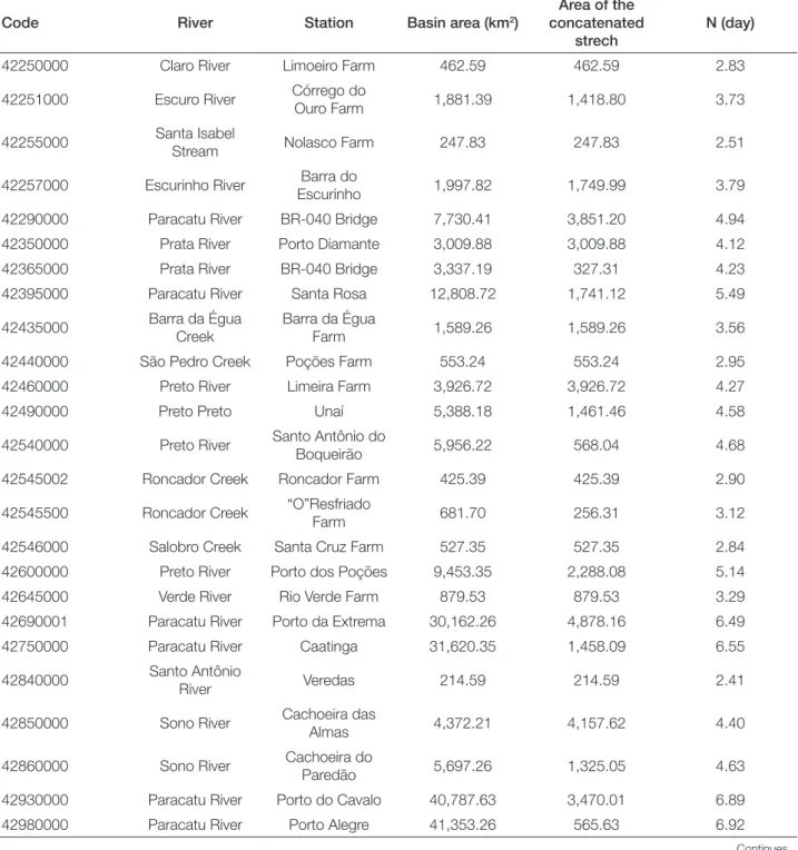
Table 2. Area data, N (days of runoff discharge influence – Linsley et al., 1979), utilized BFLW filter parameters and annual discharge of the base flow, interflow and quick flow.
Code River Station Basin area (km2)
Area of the concatenated
strech
N (day)
42250000 Claro River Limoeiro Farm 462.59 462.59 2.83
42251000 Escuro River Córrego do Ouro Farm 1,881.39 1,418.80 3.73
42255000 Santa Isabel Stream Nolasco Farm 247.83 247.83 2.51
42257000 Escurinho River EscurinhoBarra do 1,997.82 1,749.99 3.79
42290000 Paracatu River BR-040 Bridge 7,730.41 3,851.20 4.94
42350000 Prata River Porto Diamante 3,009.88 3,009.88 4.12
42365000 Prata River BR-040 Bridge 3,337.19 327.31 4.23
42395000 Paracatu River Santa Rosa 12,808.72 1,741.12 5.49
42435000 Barra da Égua Creek Barra da Égua Farm 1,589.26 1,589.26 3.56
42440000 São Pedro Creek Poções Farm 553.24 553.24 2.95
42460000 Preto River Limeira Farm 3,926.72 3,926.72 4.27
42490000 Preto Preto Unaí 5,388.18 1,461.46 4.58
42540000 Preto River Santo Antônio do Boqueirão 5,956.22 568.04 4.68
42545002 Roncador Creek Roncador Farm 425.39 425.39 2.90
42545500 Roncador Creek “O”Resfriado Farm 681.70 256.31 3.12
42546000 Salobro Creek Santa Cruz Farm 527.35 527.35 2.84
42600000 Preto River Porto dos Poções 9,453.35 2,288.08 5.14
42645000 Verde River Rio Verde Farm 879.53 879.53 3.29
42690001 Paracatu River Porto da Extrema 30,162.26 4,878.16 6.49
42750000 Paracatu River Caatinga 31,620.35 1,458.09 6.55
42840000 Santo Antônio
River Veredas 214.59 214.59 2.41
42850000 Sono River Cachoeira das Almas 4,372.21 4,157.62 4.40
42860000 Sono River Cachoeira do Paredão 5,697.26 1,325.05 4.63
42930000 Paracatu River Porto do Cavalo 40,787.63 3,470.01 6.89
42980000 Paracatu River Porto Alegre 41,353.26 565.63 6.92
The Bflow (Lyne and Hollick, 1979) and EWMA (Tularam and Ilahee, 2008) filters demonstrated a be-havior that was consistent for hydrograph separation. Chapman (1991) and Chapman and Maxwell (1996) fil-ters did not behave consistently, since in several temporal segments, they did not match the recession curve during the dry season.
With the double calibration method presented in this study, it became possible to estimate more reliably the base flow, interflow, and quick flow. The logic restrictor did not permit overestimation of the discharge, increasing the con-sistency of the results, which were coherent with Barnes (1939) manual graphic method, although the filters more reliably distinguished the difference between the base flow
Table 2. Continued
Code
Bflow Filter’s α
parameter Annual discharge by basin (m
3.s) Annual Discharge by stretch (m3.s)
Base
flow Interflow Total Base Interflow Quick Total Base Interflow Quick
42250000 0.991 0.94 3,042.14 1,883.82 471.49 686.83 3,042.14 1,883.82 471.49 686.83
42251000 0.992 0.932 10,272.11 6,495.71 1,992.04 1,784.36 7,229.97 4,611.89 1,520.55 1,097.53
42255000 0.996 0.935 1,327.04 688.61 330.45 307.99 1,327.04 688.61 330.45 307.99
42257000 0.994 0.96 9,883.07 5,762.31 2,058.92 2,061.84 8,556.03 5,073.70 1,728.47 1,753.85
42290000 0.998 0.96 37,296.61 14,536.76 11,555.12 11,204.74 17,141.43 2,278.74 7,504.16 7,358.54
42350000 0.9985 0.977 13,357.42 5,204.40 3,412.75 4,931.70 13,357.42 5,204.40 3,412.75 4,931.70
42365000 0.9985 0.95 19,107.86 6,898.34 5,380.98 6,828.54 5,750.44 1,693.94 1,968.23 1,896.84
42395000 0.998 0.97 62,072.30 26,502.71 17,505.78 18,063.81 5,667.83 5,067.61 569.68 30.53
42435000 0.9963 0.965 6,431.05 3,020.66 1,819.63 1,591.02 6,431.05 3,020.66 1,819.63 1,591.02
42440000 0.997 0.965 3,318.21 1,397.94 833.45 1,086.83 3,318.21 1,397.94 833.45 1,086.83
42460000 0.9955 0.955 21,837.01 13,473.71 4,747.93 3,615.37 21,837.01 13,473.71 4,747.93 3,615.37
42490000 0.997 0.965 28,146.95 14,271.79 6,403.81 7,471.35 6,309.94 798.08 1,655.88 3,855.98
42540000 0.997 0.97 32,653.45 16,498.50 7,085.02 9,096.94 4,506.50 2,226.71 681.21 1,625.59
42545002 0.998 0.94 1,952.24 819.43 478.42 654.39 1,952.24 819.43 478.42 654.39
42545500 0.9983 0.965 3,217.61 1,170.18 676.74 1,370.70 1,265.37 350.75 198.32 716.31
42546000 0.999 0.975 2,726.97 983.94 486.62 1,256.41 2,726.97 983.94 486.62 1,256.41
42600000 0.9974 0.975 45,070.14 20,855.40 9,701.16 14,513.58 6,472.11 2,202.78 1,452.78 2,789.53
42645000 0.999 0.935 2,567.18 711.90 1,137.07 746.55 2,567.18 711.90 1,137.07 746.55
42690001 0.9971 0.973 131,929.40 60,558.86 33,475.50 37,895.04 12,470.52 8,070.25 2,478.41 1,893.25
42750000 0.9971 0.97 136,929.60 62,092.17 34,873.59 40,026.83 5,000.20 1,533.31 1,398.09 2,131.79
42840000 0.9985 0.955 1,249.75 605.35 284.31 360.09 1,249.75 605.35 284.31 360.09
42850000 0.9984 0.975 22,337.61 6,721.81 5,745.23 9,870.57 21,087.86 6,116.46 5,460.92 9,510.48
42860000 0.9988 0.982 28,339.20 7,201.71 6,759.19 14,378.40 6,001.59 479.90 1,013.96 4,507.83
42930000 0.9976 0.976 176,576.10 74,173.48 44,433.48 57,969.10 11,307.30 4,879.60 2,800.70 3,563.87
42980000 0.998 0.978 184,740.70 78,241.19 45,384.84 61,114.66 8,164.60 4,067.71 951.36 3,145.56
and interflow. The values found for the Bflow filter param-eters were superior to the standard ones found in literature. This could mean that the pre-existing studies with this fil-ter might have overestimated the base flow, even when the subsurface flow was incorporated into their values.
As a suggestion for future studies, the methodology proposed in this article could be enhanced by algorithm developments for automatic calibration of the filters. The automatic identification of the recession curve’s inflection
point is already performed by BFI algorithm (Wahl and Wahl, 1988, 1995), and Lynsley et al.(1975) empirical for-mula is already incorporated in algorithms, such as Rora and Part (Rutledge, 1993, 1998).
47ºW
Total Flow
46ºW 45ºW 47ºW 46ºW 45ºW
16ºS
Projection Sirgas 2000
Filter Bflow (Lyne and Hollick, 1989) Gauge Stations: ANA. Reference: 1976-2001
Watershed delimitation on HCDEM based on SRTM and IBGE topography
Quick Flow
Interflow Base Flow
0
17ºS
18ºS
16ºS
17ºS
18ºS
25 50 100 150 200
km
Table 3. Specific annual discharge and discharge indexes for base flow, interflow, and quick flow in the Paracatu River Basin.
Code
Base flow index using Bar
nes (1939)
Graphic Method Index per basin Index for the str
etch
Specific discharge by basin (m 3.s/km 2)
Specific discharge by str
etch (m
3.s/km 2)
CETEC (1981) Ruralminas (1996) Base Interflow Quick Base Interflow Quick Total Base Interflow Quick Total Base Interflow Quick
42250000 – 0.61 0.62 0.15 0.23 0.62 0.15 0.23 6.58 4.07 1.02 1.48 6.58 4.07 1.02 1.48
42251000 – 0.66 0.63 0.19 0.17 0.64 0.21 0.15 5.46 3.45 1.06 0.95 5.10 3.25 1.07 0.77
42255000 – 0.64 0.52 0.25 0.23 0.52 0.25 0.23 5.35 2.78 1.33 1.24 5.35 2.78 1.33 1.24
42257000 – – 0.58 0.21 0.21 0.59 0.20 0.20 4.95 2.88 1.03 1.03 4.89 2.90 0.99 1.00
42290000 – 0.51 0.39 0.31 0.30 0.13 0.44 0.43 4.82 1.88 1.49 1.45 4.45 0.59 1.95 1.91
42350000 0.30 0.58 0.39 0.26 0.37 0.39 0.26 0.37 4.44 1.73 1.13 1.64 4.44 1.73 1.13 1.64
42365000 – – 0.36 0.28 0.36 0.29 0.34 0.33 5.73 2.07 1.61 2.05 17.57 5.18 6.01 5.80
42395000 0.32 – 0.43 0.28 0.29 0.89 0.10 0.01 4.85 2.07 1.37 1.41 3.26 2.91 0.33 0.02
42435000 – 0.57 0.47 0.28 0.25 0.47 0.28 0.25 4.05 1.90 1.14 1.00 4.05 1.90 1.14 1.00
42440000 – 0.58 0.42 0.25 0.33 0.42 0.25 0.33 6.00 2.53 1.51 1.96 6.00 2.53 1.51 1.96
42460000 – 0.74 0.62 0.22 0.17 0.62 0.22 0.17 5.56 3.43 1.21 0.92 5.56 3.43 1.21 0.92
42490000 – – 0.51 0.23 0.27 0.13 0.26 0.61 5.22 2.65 1.19 1.39 4.32 0.55 1.13 2.64
42540000 – 0.66 0.51 0.22 0.28 0.49 0.15 0.36 5.48 2.77 1.19 1.53 7.93 3.92 1.20 2.86
42545002 – – 0.42 0.25 0.34 0.42 0.25 0.34 4.59 1.93 1.12 1.54 4.59 1.93 1.12 1.54
42545500 – – 0.36 0.21 0.43 0.28 0.16 0.57 4.72 1.72 0.99 2.01 4.94 1.37 0.77 2.79
42546000 – – 0.36 0.18 0.46 0.36 0.18 0.46 5.17 1.87 0.92 2.38 5.17 1.87 0.92 2.38
42600000 0.69 0.62 0.46 0.22 0.32 0.34 0.22 0.43 4.77 2.21 1.03 1.54 2.83 0.96 0.63 1.22
42645000 0.43 0.54 0.28 0.44 0.29 0.28 0.44 0.29 2.92 0.81 1.29 0.85 2.92 0.81 1.29 0.85
42690001 – 0.58 0.46 0.25 0.29 0.65 0.20 0.15 4.37 2.01 1.11 1.26 2.56 1.65 0.51 0.39
42750000 – 0.59 0.45 0.25 0.29 0.31 0.28 0.43 4.33 1.96 1.10 1.27 3.43 1.05 0.96 1.46
42840000 – 0.60 0.48 0.23 0.29 0.48 0.23 0.29 5.82 2.82 1.32 1.68 5.82 2.82 1.32 1.68
42850000 – – 0.30 0.26 0.44 0.29 0.26 0.45 5.11 1.54 1.31 2.26 5.07 1.47 1.31 2.29
42860000 0.32 0.51 0.25 0.24 0.51 0.08 0.17 0.75 4.97 1.26 1.19 2.52 4.53 0.36 0.77 3.40
42930000 – – 0.42 0.25 0.33 0.43 0.25 0.32 4.33 1.82 1.09 1.42 3.26 1.41 0.81 1.03
The methodology developed for this study is easily replicable for other Brazilian basins, as well for those worldwide, whenever gauging station information is available. The reliability verification of its results, how-ever, does not mean that a more extensive understand-ing of the hydrological, hydrogeological, and climatic phenomena occurring at the basins is not necessary.
ACKNOWLEDGMENTS
This research was supported by the Brazilian funding agencies FAPEMIG (Fundação de Amparo à Pesquisa do Estado de Minas Gerais), FINEP (Financiadora de Estudos e Projetos), CNPq (Conselho Nacional de Desenvolvimento Científico e Tecnológico) and CAPES (Coordenação de Aperfeiçoamento de Pessoal de Nível Superior).
REFERENCES
ALBUQUERQUE, A. C. L. S. Estimativa de recarga da bacia do Rio das Fêmeas através de métodos manuais e automáticos. 2009. 101 p. Dissertação (Mestrado) – Departamento de Engenharia Florestal, Faculdade de Tecnologia, Universidade Federal de Brasília, Brasília, Distrito Federal.
ALLISON, P. D. Missing Data. Newbury Park, CA: Sage, 2002. 104 p.
AMISIGO, B. A.; VAND DE GIESEN, N. C. Using a spatio-temporal dynamic state-space model with EM algorithm to patch gaps in daily riverflow series. Hydrology and Earth System Sciences, v. 9, p. 209-224, 2005.
ANA – AGÊNCIA NACIONAL DE ÁGUAS. Manual
de Construção da Base Hidrográfica Ottocodificada da ANA. Versão 2.2. Brasília, DF, 2008. 142 p.
ANDRADE, L. M. G. Uso optimal do território de bacia hidrográfica com fundamentos no conceito de geociências agrárias e ambientais. 2007. 203 p. Dissertação (Mestrado) – Departamento de Geologia, Escola de Minas, Universidade Federal de Ouro Preto, Ouro Preto, Minas Gerais.
ASMERON, G. H. Groundwater contribution and recharge estimation in the Upper Blue Nile flows (Ethiopia). 2008. 119 p. Master of Science Thesis – International Institute for Geo-information Science and Earth Observation, Netherlands.
BARNES, B. S. The structure of discharge recession curves. Transactions of the American Geophysical Union, v. 20, p. 721-725, 1939.
BILLER, R. D. The Coal River Basin, West Virginia:
a 2009 water budget study. 2010. 74 p. Master of Science Thesis – Marshall University, Huntington, West Virginia, USA.
BRODIE, R. S.; HOSTETLER, S. A review of techniques for analysing base-flow from stream hydrographs, Proceedings of the NZHS-IAH-NZSSS 2005 Conference, 28 November–2 December, Auckland, New Zealand, 2005.
CANO, S.; ANDREU, J. Using multiple imputation to simulate time series: a proposal to solve the distance effect. Journal WSEAS Transactions on Computers, v. 9, n. 7, p. 768-777, 2010.
CARVALHO, F. E. C.; FIRMIANO, R. G.; MARTINS JUNIOR, P. P. Análise Fluviométrica de Estações em Operação na Bacia do Paracatu. Finep, Igam, Cetec. In: MARTINS JUNIOR, P. P. (Coord.) Projeto CRHA, Nota Técnica: NT- 22. Belo Horizonte, MG, 2004. 224 p.
CETEC-MG – FUNDAÇÃO CENTRO
TECNOLÓGICO DE MINAS GERAIS. II Plano de Desenvolvimento Integrado do Noroeste Mineiro: Recursos Naturais. Belo Horizonte, MG, 1981.
CHAPMAN, T. G. A comparison of algorithms for stream flow recession and baseflow separation.
Hydrological Process, v. 13, n. 5, p. 701-714, 1999. CHAPMAN, T. G. Comment on evaluation of automated techniques for base flow and recession analyses, by RJ Nathan and TA McMahon. Water Resources Research, v. 27, n. 7, p. 1783-1784, 1991.
COMBALICER, E. A.; LEE, S. H.; AHN, S.; KIM, D. Y.; IM, S. Comparing groundwater recharge and base flow in the Bukmoongol small-forested watershed, Korea. Journal of Earth System Science, v. 117, n. 5, p. 553-566, 2008.
CORZO, G.; SOLOMATINE, D. Baseflow separation techniques for modular artificial neural modelling flow forecasting. Hydrological Sciences – Journal des Sciences Hydrologiques, v. 52, n. 3, 2007.
DEMPSTER, A.; LAIRD, N.; RUBIN, D. Maximum likelihood from incomplete data via the EM algorithm.
Journal of the Royal Statistical Society, Series B, v. 39, n. 1, p. 1-38, 1977.
DILLON, P. Future management of aquifer recharge.
Hydrogeology Journal, v. 13, p. 313-316, 2005. DOI: 10.1007/s10040-004-0413-6.
DOLEZAL, F.; KVÍTEK, T. The role of recharge zones, discharge zones, springs and tile drainage systems in peneplains of central European highlands with regard to water quality generation processes. Physics and Chemistry of the Earth, v. 29, p. 775-785, 2004. ENDERS, C. K. Applied Missing Data Analysis.
New York: The Guilford Press, 2010. 375 p.
EUCLYDES, H. P. (Coord.). Ferramenta para o planejamento e gestão de recursos hídricos nos Estado de Minas Gerais – HIDROTEC. Viçosa, MG: Departamento de Engenharia Agrícola da Universidade Federal de Viçosa; Brasília, DF: Ministério do Meio Ambiente; Belo Horizonte, MG: RURALMINAS. 2004. Disponível em: <www.ufv.br/dea/hidrotec>. Acesso em: 14/02/2013.
GHANBARPOUR, M. R.; TEIMOURI, M.; GHOLAMI, S. H. Comparison of base flow estimation methods based on hydrograph separation (case study: Karun Basin) JWSS – Isfahan University of Technology, v. 12, n. 44, p. 1-13, 2008.
GONZALES, A. L.; NONNER, J.; HEIJKERS, J.; UHLENBROOK, S. Comparison of different base flow separation methods in a lowland catchment. Hydrology and Earth Sciences Discussions, v. 6, p. 2483-3515, 2009. GREGOR, M. BFI+ 3.0 User’s Manual. HydroOffice. Software Package for Water Sciences. State Geological Institute of Dionyz Stur, Bratslava, Czech Republic, 2010. 21 p.
HALFORD, K. J.; MAYER, G. C. Problems associated with estimating ground water discharge and recharge from streamflow-discharge records. Ground Water, v. 38, n. 3, p. 331-342, 2000.
HARTLEY, H. Maximum likelihood estimation from incomplete data. Biometrics, v. 14, p. 174-194, 1958. HOLTSCHLAG, D. J. A generalized estimate of ground-water-recharge rates in the Lower Peninsula of Michigan. U.S. Geological Survey water-supply paper 2437. 1997. 44 p.
IGAM – INSTITUTO MINEIRO DE GESTÃO DAS ÁGUAS. Plano Diretor de Recursos Hídricos do Rio Paracatu: Resumo Executivo. Governo de Minas Gerais. Comitê da Sub-baciaHidrográfica do Rio Paracatu. Belo Horizonte: Instituto Mineiro de Gestão das Águas, 2006. 384 p.
JOHNSON, G. S.; SULLIVAN, W. H.; COSGROVE, D. M.; SCHIMIDT, R. D. Recharge of the Snake River Plain Aquifer: Transitioning from Incidental to Managed. Paper Nº 98010, Journal of the American Water Resources, 1999.
KIRCHNER, J. W. A double paradox in catchment hydrology and geochemistry. Hydrological Processes, v. 17, p. 871-874, 2003.
LAROCQUE, M.; FORTIN, V.; PHARAND, M. C.; RIVARD, C. Groundwater contribution to river flows – using hydrograph separation, hydrological and hydrogeological models in a southern Quebec aquifer.
Hydrology and Earth System Sciences Discussions, v. 7, p. 7809-7838, 2010. Disponível em: <www.hydrol-earth-syst-sci-discuss.net/7/7809/2010/>. Acesso em: 14 fev. 2013. doi:10.5194/hessd-7-7809-2010.
LATUF, M. O. Mudanças de Uso do Solo e Comportamento Hidrológico nas Bacias do Rio Preto e de Entre-Ribeiros.
2007. 103 p. Dissertação (Mestrado) – Programa de Pós-Graduação em Engenharia Agrícola, Universidade Federal de Viçosa, Viçosa, MG.
LIM, K. J.; ENGEL, B. A.; TANG, Z.; CHOI, J.; KIM, K. S.; MUTHUKRISHNAN, S.; TRIPATHY, D. Automated Web GIS based Hydrograph Analysis Tool, WHAT. Journal of the American Water Resources Association, p. 1407-1416, 2005.
CHOI, J.; YOO, D. S. Development of Optimization Module in the WHAT System for Accurate Hydrograph Analysis and Model Application. In: ASAE ANNUAL MEETING072022, American Society of Agricultural and Biological Engineers, 2007.
LIM, K. J.; PARK, Y; KIM, J.; SHIN, Y. C.; KIM, N. W.; KIM, S. J.; JEON, J. H.; ENGEL, B. A. Development of genetic algorithm-based optimization module in WHAT system for hydrograph analysis and model application. Computers & Geosciences, v. 36, p. 936-944, 2010. DOI: 10.1016/j.cageo.2010.01.004.
LYNE, V.; HOLLICK, M. Stochastic time-variable rainfall-runoff modeling. Institute of Engineers Australia National Conference, p. 89-93, 1979.
LYNSLEY, R. K.; KOHLER, M. A.; PAULHUS, J. L. H.; WALLACE, J. S. Hydrology for Engineers, 2nd edition. New York: McGraw Hill, 1975.
MARTINS JUNIOR, P. P. (Coord.). Projeto GZRP – Gestão de Zonas de Recarga de Aqüíferos Partilhadas entre as Bacias de Paracatu, São Marcos e Alto Paranaíba. Cetec/Fapemig - 2007-2009. Fundação Centro Tecnológico de Minas Gerais, Belo Horizonte, Minas Gerais. Relatório Final em 2009.
MARTINS JUNIOR, P. P. Projeto CRHA – Conservação de recursos hídricos no âmbito de gestão agrícola de bacias hidrográficas. MCT/Finep/CT-Hydro 2002-2006. Fundação Centro Tecnológico de Minas Gerais, Belo Horizonte, Minas Gerais. Relatório Final em 2006.
MCMAHON, T. A.; MEIN, R. G. River and Reservoir Yield. Littleton: Water Resources Publication, 1986. 368 p.
MOREIRA, M. C. Gestão de Recursos Hídricos: Sistema Integrado para otimização da Outorga de Uso da Água. 2006. 94 p. Tese (Doutorado) – Programa de Pós-Graduação em Engenharia Agrícola, Universidade Federal de Viçosa, Viçosa, Minas Gerais.
MOURÃO, M. A. A. (Coord.). Caracterização Hidrogeológica da Microrregião de Unaí. Projeto São Francisco. Província Mineral Bambuí (MG). Brasília: Companhia de Pesquisa de Recursos Minerais, Serviço Geológico do Brasil, Ministério das Minas e Energia, 2001. 86 p.
MULHOLLAND, D. S. Geoquímica Aplicada à
Avaliação de Qualidade de Sistemas Aquáticos da
Bacia do Rio Paracatu (MG). 2009. 95 p. Dissertação (Mestrado) – Instituto de Geociências, Universidade de Brasília, Brasília, Distrito Federal.
MÜLLER, I. I.; MARCHAND, C. M.; KAVISKI, E. Análise de Estacionariedade de Séries Hidrológicas na Bacia Incremental de Itaipu. Revista Brasileira de Recursos Hídricos, v. 3, n. 4, p. 51-71, 1998.
NATHAN, R. J.; MACMAHON, A. A. Evaluation of automated techniques for base flow and recession analyses.
Water Resources Research, v. 26, n. 7, p. 1465-1473, 1990. NOVAES, L. F. Modelo para a Quantificação da Disponibilidade Hídrica na Bacia do Paracatu. 2005. 104 p. Tese (Doutorado) – Programa de Pós-Graduação em Engenharia Agrícola, Universidade Federal de Viçosa, Viçosa, Minas Gerais.
NUNES, H. T.; NASCIMENTO, O. B. Base de Dados Meteorológicos. Belo Horizonte: Nota Técnica NT-CRHA 17/2004. In: MARTINS JUNIOR (Coord.).
Projeto CRHA. Memória Técnica da Fundação CETEC, 2004. 40 p.
PETERS, E.; VAN LANEN, H. A. J. Separation of base flow form streamflow using groundwater levels – illustrated for the Pang catchment (UK). Hydrological Processes,v. 19, p. 921-936, 2005.
PRESTI, R. L.; BARCA, E.; PASSARELLA, G. A methodology for treating missing data applied do daily rainfall data in the Candelaro River Basin (Italy).
Environmental Monitoring and Assessment, v. 160, p. 1-22, 2010. DOI: 10.1007/s10661-008-0653-3.
PRUSKI, F. F.; RODRIGUEZ, R. D. G.; NOVAES, L. F.; SILVA, D. D. D; RAMOS, M. M.; TEIXEIRA, A. F. Impacto das vazões demandadas pela irrigação e pelos abastecimentos animal e humano, na Bacia do Paracatu. Revista Brasileira de Engenharia Agrícola e Ambiental, v. 11, n. 2, p. 199-210, 2007.
RAMOS, M. L. S.; PAIXÃO, M. M. O. M. Disponibilidade Hídrica de Águas Subterrâneas – Produtividade de Poços e Reservas Explotáveis dos Principais Sistemas Aqüíferos. 41 p. In: ANA –
AGÊNCIA NACIONAL DE ÁGUAS. Plano Diretor
de Recursos Hídricos da Bacia do Rio São Francisco.
Brasília: Ministério do Meio Ambiente, 2004.