ISSN 0103-8478
Gabriel Constantino BlainI
Modeling extreme minimum air temperature series under climate change conditions
Modelagem de séries de temperatura mínima extrema sob condições de alterações climáticas
ABSTRACT
Considering the presence of non-stationary components, such as trends, in the extreme minimum air temperature series available from three locations of the State of São Paulo-Brazil, the aim of this research was to describe the probabilistic structure of this variable by using a non-stationary model (based on the general extreme value distribution; GEV model) in which the parameters are estimated as a function of time covariate. The Mann-Kendall test has proven the presence of significant increasing trends in all analyzed series. Furthermore, according to the Pettitt (changing-point) test, 1991 is the initial year of these trends (in the three locations). The applied selection criteria indicated that a GEV model in which the location parameter is estimated as a function of time is recommended to describe the probability structure of the variable under evaluation. The others two parameters of this model remained time-independent. According to this non-stationary model, the detected trends in the climate conditions of these locations have shown the same rate of change (0.04ºC per year).
Key words: time-dependent model, probability function,
non-stationary approach.
RESUMO
Considerando a presença de componentes não estacionárias, tais como tendências, nas séries de temperatura do ar mínima extrema, disponíveis a partir de três localidades do Estado de São Paulo, o objetivo do trabalho foi descrever a estrutura probabilística dessa variável, utilizando um modelo não estacionário (baseado na distribuição geral dos valores extremos; modelo GEV) em que os parâmetros são estimados em função da co-variável tempo. O teste de Mann-Kendall comprovou a presença de significativas tendências de elevação
em todas as séries analisadas. Em adição, de acordo com o teste de Pettitt (teste de ponto de mudança), 1991 é o ano inicial dessas tendências (nas três localidades). Os critérios de seleção aplicados indicaram que um modelo GEV, em que o parâmetro de localização é estimado como uma função do tempo, é recomendado para descrever a estrutura probabilística da variável sob análise. Os demais parâmetros desse modelo permaneceram independentes do tempo. De acordo com esse modelo não estacionário, as tendências detectadas nas condições climáticas dessas localidades apresentam a mesma taxa de alteração (0,04ºC por ano).
Palavras-chave: modelo dependente do tempo, função
probabilidade, abordagem não estacionária.
INTRODUCTION
Parametric distributions have been used to assess the probability of occurrence of extreme minimum air temperature values that may cause death of plant tissues. For instance, ASTOLPHO et al. (2004) used a particular case of the general extreme value distribution (GEV) to describe the probabilistic structure of the annual extreme minimum air temperature series (Tminabs) available from the weather station of Campinas, State of São Paulo, Brazil. Working under an agrometeorological framework, the main focus of these authors was to evaluate the probability of occurrence of frosts that may cause death of the plant tissues.
Considering that a basic assumption from the extreme value theory (TVE) is that the distribution of the maximums of independent and identically distributed random variables, converge to one of the particular cases of the GEV (COLES, 2001), and also based on the assumption that the GEV has all the flexibility of its three particular cases NADARAJAH & CHOI, 2007). BLAIN (2010) used the GEV distribution to assess the probability of occurrence associated with Tminabs values (1948-2007), observed in six regions of the State of São Paulo.
The GEV is a three parameter function in which the probability of occurrence of an extreme event, observed in any time (t), can be described as Pr{X zt}=GEV(zt; µ, , ); where µ, , are, respectively,
the parameters of location, scale and, shape. Since the parameters of this distribution are time-independent, the use of the GEV(µ, , ) model is frequently called “the stationary approach”. Consequently, once a stationary GEV model is fitted from a time span (from 1951 to 2010, for e.g.), it is assumed that the values of µ, , will remain the same during the next (t) years. However, according to COLES (2001), FELICI et al. (2007) and, FURIÓ & MENEU (2010), if a significant trend is detected in a meteorological data sample (composed by extreme values), the assumption that the probabilistic structure of this series does not change over the time may no longer be supported. Consequently, under non-stationary climate conditions, the use of a stationary GEV model may underestimate or overestimate the probability of occurrence associated with an extreme (agro) meteorological event.
It is worth emphasizing that the Intergovernmental Panel on Climate Change (IPCC 2007) indicates that the intensity and the frequency of extreme meteorological events (such as extreme low temperatures) will change due to the global warming. In addition, the IPCC (2007) also states that the recent increases of the global air temperature already have perceptible impacts on many natural systems. After evaluating the presence of trends in several indices of daily air temperature for South America, VINCENT et al. (2005) states that although no consistent change has been observed in indices estimated from maximum temperature data, significant trends were verified in indices based on minimum temperatures. These last considerations have allowed us to work under the hypothesis that the use of a time-dependent GEV model (compared with the use of a stationary GEV model) provides a better assessment of the probability of occurrence associated with Tminabs data. Thus, the aim of this study was to describe the probabilistic
structure of Tminabs series by using a non-stationary GEV model in which the parameters are estimated as a function of time covariate.
MATERIAL AND METHODS
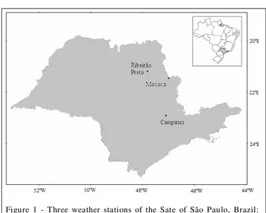
Annual extreme daily minimum air temperature data were used from the weather stations of Campinas (22º56’S; 46º54’W; 690m), Mococa (21º32’S; 46º59’W; 665m) and, Ribeirão Preto (21º11’S; 47º48’W; 621m), between 1951 and 2010. These weather stations are situated in the State of São Paulo-Brazil (Figure 1). The data sample was obtained from the Instituto Agronômico (IAC/APTA/SAA).
The Mann-Kendall trend test (MK; KENDALL & STUART, 1967) and the Pettitt test (PETTITT, 1979) were used in order to evaluate the presence of trends components in each one of the Tminabs series. The null hypothesis (Ho) associated with these both tests, assumes that the sample is free from trends (the absence of significant serial correlation is also assumed). The Ho is usually rejected if the probability of occurrence of type I error (p-value) is less than or equal to 0.05. Positive (negative) MK values are representative of increasing (decreasing) trends. Following BLAIN (2011), the Pettitt test was used to detect the initial year of the climate trends observed in each one of the Tminabs series. The p-value associated with this test was also estimated. The Durbin-Watson test was used in order to evaluate the presence of significant correlation in the Tminabs series. P-values (associated with this former test) greater than 0.05, were taken as an evidence that the absence of significant serial correlation may be assumed. Following COLES (2001), EL ADLOUNI et al. (2007), CANON (2010) and, FURIÓ & MENEU (2010), a non-stationary GEV model may be described by the following probability density function:
only if > 0...(1). In order to incorporate the presence of climate trends in the modeling of the Tminabs series, the following GEV models are proposed. Model 1 (The stationary model): GEV(µt=µ, t= , t= ); Model 2 (Non
stationary model with µo and ß being, respectively, the
intercept and the rate of change): GEV(µt=µo + ßt,
t= , t= ); Model 3 (Non stationary model with µ’o,
o, and, ß’ being, respectively, the intercept and the
rate of change of each time-dependent parameter). The exponential function is used to ensure a positive value for the scale parameter: GEV(µt=µ’o + ß’t, t= exp ( o + t),
ξ ξ
t= ); Model 4 (Non stationary model with µ”o, ’o,
o and ß”, ’, being, respectively, the intercept and the
rate of change of each time-dependent parameter): GEV(µt=µ”o + ß”t, ’t= exp( ’o + ’t), t = o + t). It is
worth emphasizing that model 1 can be seen as a particular case of model 2. Consequently, models 1 and 2 are particular cases of model 3. Finally, these three models can be seen as particular cases of model 4. Following COLES (2001) the parameters of equation 1 were estimated by using the method of maximum likelihood (hereafter, these estimative will be represented by the italic form of each parameter; µ, , ). In addition,
it is worth emphasizing that according to COLES (2001), although the TVE is often related to the description of the behavior of the maximum values observed in a data sample, its approach is equally applicable to the evaluation of the smallest values observed in a data sample. In this case, it is only necessary to transform the variables x into –x and, consequently, –µ into µ.
Following BURNHAM & ANDERSON (2004), the model selection (equations 2 and 3) was initially based on ‘Akaike’s information criteria’. AIC(Modeli)= -21(Modeli) + 2K for i=1 to 4...(2)
(Modeli)=AIC(Modeli)= minimumAIC(Modeli)...(3)
Where k is the number of parameters of each (i) Model and, l(.) is the maximized log likelihood function of Modeli.
As described in FELICI et al. (2007), all models with (.) 2 were initially selected. After this initial step, it is worth emphasizing that according to EL ADLOUNI et al. (2007), the most general model is frequently the best to represent the data sample under analysis. However, since the uncertainty in quantiles
estimate increases as the number of parameters to be estimated increases, these authors also indicates that when the differences between two GEV models are not significant, it is better to use the simplest one. Following FELICI et al. (2007), it was applied equation 4 (the deviance statistic; D) in order to evaluate the differences between the models selected by equations 2 and 3.
D= 2(11(Modelj)-10(Modeli)) for j>i; Mi Mj ...(4)
The statistical significance of D can be evaluated by the chi-square distribution with degrees-of-freedom equal to the difference in the dimensionality of the modelsp-values equal or less than 0.05 were seen as an evidence that Modelj is better than Modeli
in explaining the data variation (COLES, 2001 and EL ADLOUNI et al., 2007). Finally, the adequacy of the selected model was evaluated from goodness-of-fit procedures that give special focus for the lower tail of the distributions. In this view, the quantil-quantil plot (QQ) and the percentil-percentil plot (PP) were used in order to compare the observed data and the fitted GEV model. However, a natural consequence of adopting a time-dependent model is that the data cannot be considerate as independent and identically distributed. Thus, before plotting the QQ and PP, the data were transformed in order to ensure that each point has the same joint distribution. This transformation was achieved by adopting the procedure described in COLES (2001), considering a standardized variable (Xt)
defined in equation 5 (with a distribution given by equation 6).
……….(5)
Figure 1 - Three weather stations of the Sate of São Paulo, Brazil: Campinas (22°54’S, 47°05’, 669m), Mococa (21°28’S, 47°01’, 665m) and, Ribeirão Preto (21°11’S, 47°48’, 620m).
ξ ξ
ξ
ξ
) (
) ( ) ( 1 log ) ( 1
t t X t t
X t
t
ξ
Pr{X(t) x} = exp{-exp(-x)}………...(6) Denoting the ordered values of xtby
x(1)….x(m), a PP plot may be build by the pairs {i/(m+1),
exp(-(exp(-x(i))); i=1,…m}, while the QQ plot may consist
of the pairs { x(i), -log(-log(i/(m+1)))); i=1,…m}. Further
information related to the PP and QQ plots can be found in COLES (2001) and FELICI et al. (2007). The parameters of equation 1 were estimated by using the R software. All other procedures were calculated by using the Matlab software.
RESULTS AND DISCUSSION
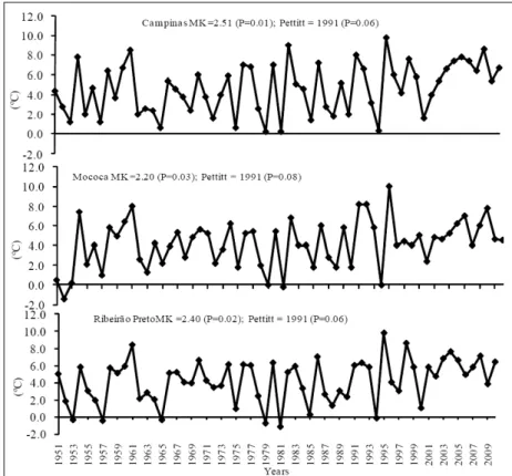
The Durbin-Watson test indicated the absence of significant serial correlation in the three series. The P-values associated with this test were always greater than 0.05. The MK test indicates the presence of significant increasing trends in all analyzed series (Figure 2). In addition, it is worth emphasizing that, according to the Pettitt test, 1991 is the initial year of these trends (in the three locations; Figure 2). Thus, based on the results of both tests, there were enough evidences to support the hypothesis that the presence of climate trends in the Tminabs series may no longer be neglected. Under a statistical framework, we may
not assume that the Tminabs data are independent and identically distributed. The probabilistic structure of this variable does change with time. Future studies should investigate if the results shown in figure 2 (especially the initial year of the trend) can be verified in others weather stations or regions (if available) of the State of São Paulo.
The results depicted in figure 2 associated with the IPCC (2007) statements (previously described), support the hypothesis that adopting a GEV non-stationary model will result in a more feasible description (compared with the stationary approach) of the probability of occurrence associated with future Tminabs values. This last consideration is supported by equations 2 and 3, since the quantities , estimated under the stationary approach (Model 1), were always greater than 2 ( =4.05 – Campinas, =4.07 – Mococa and, =3.36 – Ribeirão Preto). Under the non-stationary approach (Models 2, 3 and 4), values of <2 were obtained by the Models 2 and 4 (Campinas) and Models 2 and 3 (Mococa and Ribeirão Preto). Thus, these last models were subjected to the analysis based on equation 4. As indicated by the deviance statistic, no significant improvement was achieved when the most general models were used in the three series under evaluation.
Figure 2 - Extreme minimum air temperature series available from three locations of the State of São Paulo, Brazil (1951-2010). The Mann-Kendall (MK) trend test and Pettitt (changing point) test are also shown.
The p-values associated with the quantity D (Models 4-2; Campinas and, Models 3-2; Mococa and Ribeirão Preto) were always much greater than 0.05. Thus, under the principle of parsimony (‘obtaining the simplest model possible’; COLES, 2001) the Model 2 was chosen for building the Y-axis of the PP and QQ plots.
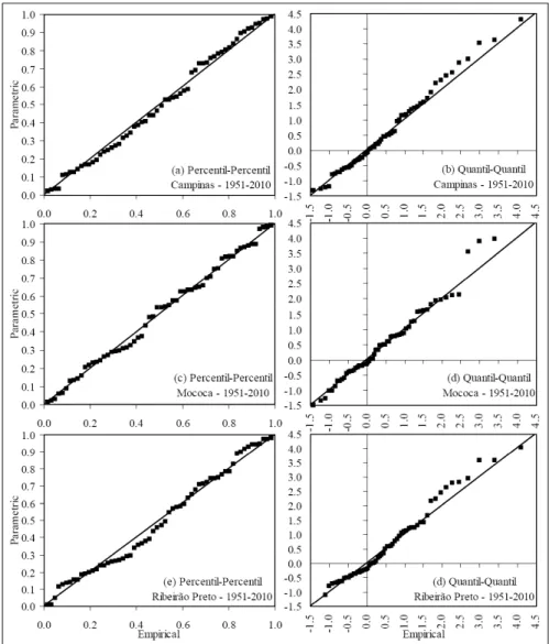
The small displacement of the Cartesian points in both PP and QQ plots (Figure 3) supports the decision of using Model 2 to assess the probability of occurrence associated with the Tminabs values in the three analyzed series. The parameters of this model are:
µt=4.08 + 0.044t, t= =2.394, t= = -0.306 (Campinas;
the standard errors are, respectively, 0.645, 0.018, 0.250 and, 0.109); µt=3.62+0.043t, t= =2.305, t= = -0.325
(Mococa; the standard errors are, respectively, 0.620, 0.017, 0.237 and, 0.090) and, µt=3.89+0.041t, t= =2.260,
t= = -0.190 (Ribeirão Preto; the standard errors are,
respectively, 0.630, 0.017, 0.235 and, 0.102). It is worth emphasizing that the annual rate of change of the location parameter is practically the same for the three locations (+0.04 per year; approximately). This last consideration is consistent with the results obtained by VINCENT at al. (2005) in the sense that the coldest night of the year is getting warmer throughout the South America. In order to evaluate a possible use of Model 2, it was estimated the cumulative probability associated with Tminabs values equal or lower than 3, 2 and 1ºC. For more information about the relationship between Tminabs values and frost occurrence see SENTELHAS et al. (1995).
As expected, the probabilities of occurrence associated with the values shown in table 1 tend to
Figure 3 - Evaluating the use of a nonstationary GEV model (the location parameter depends on time) for describing the probabilistic structure of extreme minimum air temperature series available from three locations of the State of São Paulo, Brazil.
ξ
ξ ξ
ξ
decrease over the years 2020-2050. In this view, it is worth emphasizing that the period of 2001-2010 is the only one 10-year time span (considering the years of 1951-2010) in which no value lower than 3ºC was observed (Figure 1). In fact, the lowest air temperature value observed during these last 10 years was 3.8ºC (2009; Ribeirão Preto). Furthermore, the results presented in this study, have given us enough (statistical) evidences to support the hypothesis that the risk of crop damage caused by frosts in these three regions is declining over the years. After verifying this last feature, it becomes interesting to recall that according to ALEXANDER et al. (2006), there is a positive shift in the distributions of daily minimum air temperature throughout the globe.
Finally, it is worth mentioning that since the presence of climate trends were detected in the analyzed series, the non-stationary approach proposed in this study, can be seen as an evolution in the stochastic modeling of these datasets. However, it is also worth emphasizing that all proposed models are linear or log-linear equations in which the dependence of the parameters on the covariates had to be specified
a priori (CANNON, 2010). Although several authors
also adopt this approach (COLES, 2001; El ADLOUNI et al., 2007; FELICI et al., 2007 and, FURIÓ & MENEU, 2010), CANNON (2010) specifies the parameters of the GEV based on a probabilistic extension of the multilayer perceptron neural network. Consequently, the framework, proposed by CANNON (2010), can be seen
as an important future alternative to overcome this linear approach, improving the results achieved in this study.
CONCLUSION
A nonstationary GEV model in which the location parameter is estimated as a function of time is recommended to describe the probabilistic structure of extreme minimum air temperature series available from three weather station of the State of São Paulo (Campinas, Mococa and, Ribeirão Preto). The need of using this non-stationary approach is a consequence of the presence of increasing trends in these three meteorological data samples.
The detected trends in the climate conditions of these locations have shown the same rate of change (0.04ºC per year). This coherence was also observed in the initial year of the trends (1991).
REFERENCES
ALEXANDER, L.V. et al. Global observed changes in daily climate extremes of temperature and precipitation. Journal of Geophysical Research, v.111, 2006. Available from: <http://www.agu.org/journals/jd/jd0605/2005JD006290/>. Accessed: Jan 12, 2011. doi: 10.1029/2005JD006290. ASTOLPHO, F. et al. Probabilidades mensais e anuais de ocorrência de temperaturas mínimas do ar adversas à agricultura na região de Campinas (SP) de 1891 a 2000. Bragantia, v.63, p.141-147, 2004. Available from: <http://www.scielo.br/ s c i e l o . p h p ? s c r i p t = s c i _ a r t t e x t & p i d = S 0 0 0 6 -87052004000100014&lng=en&nrm=iso>. Accessed: Jan 12, 2011. doi: 10.1590/S0006-87052004000100014.
BLAIN, G.C. Detecção de tendências monótonas em séries mensais de precipitação pluvial do estado de São Paulo. Bragantia, v.63, p.1027-1033, 2011. Available from: <http:/ /www.scielo.br/scielo.php?script=sci_arttext&pid=S0006-87052010000400031&lng=en&nrm=iso>. Accessed: Jan 12, 2011. doi: 10.1590/S0006-87052010000400031.
BLAIN, G.C. Precipitação pluvial e temperatura do ar no Estado de São Paulo: periodicidades, probabilidades associadas, tendências e variações climáticas. 2010. 194f. Tese (Doutorado em ciências) – Universidade de São Paulo, Piracicaba, SP.
BURNHAM, K.P.; ANDERSON, D.R. Multimodel inference: understanding AIC and BIC in model selection. Sociological Methods Research, v.33, p.261-304, 2004. Available from: <http://smr.sagepub.com/content/33/2/261>. Accessed: Jan 12, 2011. doi: 10.1177/0049124104268644.
CANNON, A.J. A flexible nonlinear modeling framework for nonstationary generalized extreme value analysis in hydroclimatology. Hydrological Process, v.24, p.673-685, 2010. Available from: <http://www.eos.ubc.ca/~acannon/ GEVcdn/GEVcdn-paper.pdf>. Accessed: Jan 12, 2011. doi: 10.1002/hyp.7506.
Table 1 - Probabilities of occurrence associated with extreme minimum air temperature values in three locations of the State of São Paulo, Brazil. The values were estimated by using the nonstationary model GEV (xt;
μt, σ, ξ), considering the 95% confidence interval.
---Campinas---Year
3ºC 2ºC 1ºC
COLES, S. An introduction to statistical modeling of extreme value. London: Springer 2001. 208p.
EL ADLOUNI, S. et al. Generalized maximum likelihood estimators for the nonstationary generalized extreme value model. Water Resources Research, v.43, 2007. Available from: <http:/ /www.agu.org/journals/ABS/2007/2005WR004545.shtml>. Accessed: Jan. 12, 2011. doi: 10.1029/2005WR004545. FELICI, M. et al. Extreme value statistics of the total energy in an intermediate-complexity model of the midlatitude atmospheric jet. Part II: trend detection and assessment. Journal of the Atmospheric Science, v.64, p.2159-2175, 2007. Available from: <http://journals.ametsoc.org/doi/pdf/ 10.1175/JAS4043.1>. Accessed: Jan 12, 2011. doi: 10.1175/ JAS4043.1.
FURIÓ, D.; MENEU, V. Analysis of extreme temperatures for four sites across Peninsular Spain. Theoretical Applied Climatology, v.24, p 83-99 2010. Available from: <http:// www.spr i ngerl i nk . com/ cont ent/ q6 v7 l 1 85 4 2 5 4 0 3 70 / > . Accessed: Jan 12, 2011. doi: 10.1007/s00704-010-0324-5. IPCC. Climate change 2007: the physical science basis, contribution of working group I to the Fourth Assessment Report of the Intergovernmental Panel on Climate Change. HOUGHTON, J.T. (Ed.). Geneva: Cambridge University, 2007. 996p.
KENDALL, M.G.; STUART, G. The advanced theory of statistics. 2.ed. Londres: Charles Griffin & Company, 1967. V.2, 690p.
NADARAJAH, S.; CHOI, D. Maximum daily rainfall in South Korea. Journal of Earth System Science, v.116, p.311-320, 2007.
PETTITT, A.N. A non-parametric approach to the change-point problem. Journal of the Royal Statistical Society, v.28, p.126-135, 1979. Disponível em: <http://www.jstor.org/pss/2346729>. Acesso em: 19 nov. 2010.
SENTELHAS, P.C. et al. Estimativa da temperatura mínima de relva e da diferença de temperatura entre o abrigo e a relva em noites de geada. Bragantia, v.54, p.437-445, 1995. Available from: <http://www.scielo.br/scielo.php?script=sci_arttext&pid=S0006-87051995000200023&lng=en&nrm=iso>. Accessed: Jan 12, 2011. doi: 10.1590/S0006-87051995000200023.