Atmospheric dynamics of Venus using space based observations and cloud tracking techniques

(1)

UNIVERSIDADE DE LISBOA

FACULDADE DE CIÊNCIAS

DEPARTAMENTO DE FÍSICA

Atmospheric Dynamics of Venus using Space based

observations and cloud tracking techniques

Daniela Cortes Espadinha

Mestrado em Física

Especialização em Astrofísica e Cosmologia

Dissertação orientada por:

Doutor Pedro Machado

(2)

Acknowledgments

Astronomy and Astrophysics were a passion and a dream since I first got a book on the Solar System when I was at the very young age of three. My first memories of space came from that little book, which I requested my parents to read to me over and over again. For five years now, and especially since I began my Master’s degree on Astrophysics and Cosmology, that dream of working on what I loved the most progressively became a reality. The support of many people along the way was a crucial factor for my success and for all the work that I have done throughout this time.

Firstly, I would like to thank my parents, Clarinda Margarida Morais Cortes and Jos´e Jo˜ao Mendes Espadinha. They always supported my decision of following my dreams, even if we some time did not see eye to eye, but I know they always had my best interest in mind. In fact, they were the ones that opened many doors in my way and that made continuous efforts to raise and teach me the basics of a fulfilling life. They were the ones who still offered me all the support I needed when I left my small town’s home and travelled to the capital of Lisbon to study. I only hope I can make them proud.

I also want to thank my sister Adelaide, for her endless support and for coming with me to the bustling Lisbon. I never felt alone in my endeavours and surely I had someone always by my side whom I could trust and who was a shoulder to cry on if needed. And when those moments when all we think is giving up and that continuing is impossible, I want to thank my boyfriend, Joseph Wilkinson, for making me realise that I should keep giving my dream a chance and rely more on myself and my decisions.

I will always thank my friends Ana Carvalho and Inˆes Costa, for all their support, the way they helped me grow and all they taught me. Because of them I am a much better person today and I just hope that I also contributed somehow to their lives so that our relationship can last. I cannot leave unsaid a special thanks to the team working with me at IA (Institute of Astrophysics and Space Sciences) for welcoming me with open arms, and for all the advice and help given since I started my career.

And last but not the least, I am grateful to my supervisor Pedro Mota Machado, he was not only a teacher but also a guide and a friend. I could never imagine to have such a generous and helpful person so early in my career. He trusted in my abilities and competence, gave me opportunities to start fulfilling my research and, most important of all, taught me the beauty of being a scientist and the value of teamwork.

(3)

Resumo

O planeta mais próximo da Terra e o segundo objecto mais brilhante no céu nocturno é Vénus. Nomeado em honra da deusa romana do amor e da beleza, o nosso vizinho e planeta “irmão” partilha muitas caracter´ısticas semelhantes às da Terra, nomeadamente a massa, a densidade e o tamanho. No entanto, Vénus e a Terra não podiam ser planetas mais diferentes. As condi¸cões prop´ıcias à vida, como esta é conhecida na Terra, contrastam fortemente com as condi¸cões hostis que Vénus apresenta. Exemplos destas caracter´ısticas incluem a temperatura superficial: no nosso planeta a temperatura ronda os 15◦C mas em Vénus chega aos 460◦C,

uma temperatura capaz de derreter chumbo na superf´ıcie Venusiana. Em Vénus, a pressão atmosférica chega a ser aproximadamente 90 bar, ou seja, a pressão correspondente à verificada a 1 km de profundidade nos oceanos terrestres e a sua massa atmosférica é cerca de 92 vezes a massa da atmosfera terrestre. O efeito de estufa descontrolado existente em Vénus é outra caracter´ıstica que distingue os dois planetas. Este fenómeno é causado principalmente devido à quantidade de CO2 que, em Vénus, representa 96% da totalidade da atmosfera ao invés de que, na Terra, esta quantidade n˜ao ultrapassa os 0.034%. Estas caracter´ısticas s˜ao consequências directas das diferentes composi¸cões qu´ımicas, massas atmosféricas e moléculas condensáveis. Todo este cenário contrasta com a hipótese de que ambos os planetas se formaram na mesma altura de evolu¸cão do sistema solar, com as mesmas condi¸cões iniciais, e a partir da mesma nuvem proto-estelar mas, como é poss´ıvel concluir, seguiram evolu¸cões diferentes entre si. Além das condi¸cões superficiais e atmosféricas já referidas, existem ainda outras caracter´ısticas que tornam a Terra e Vénus tão diferentes. Vénus é um planeta com rota¸cão retrógada cujo per´ıodo ´

e de 243 dias terrestres o que, leva a que um dia solar em Vénus seja de 117 dias terrestres. Seria de esperar que a atmosfera Venusiana acompanhasse este per´ıodos de rota¸cão, o que não se verifica.

A atmosfera de Vénus está num estado denominado de super-rota¸cão. Isto advém do facto de que esta apresenta um per´ıodo de rota¸cão de cerca de 4.4 dias terrestres, onde o seu movimento acompanha o movimento de rota¸cão retrógado do planeta. Na região equatorial, os ventos podem alcan¸car velocidades superiores a 100 m/s, ou seja, velocidades superiores a 360 km/h. A caracteriza¸cão completa e pormenorizada deste fenómeno torna-se então um factor de alta importância na compreensão dos mecanismos que criam e regem as atmosferas planetárias.

A densa camada de nuvens que envolve a atmosfera Venusiana é composta na sua maior parte por got´ıculas de ácido sulfúrico e um composto ainda por identificar mas que absorve fortemente a radia¸cão ultravioleta no topo da mesma. Os contrastes resultantes da interaçcão da radia¸cão solar e estes constituintes criam padrões nas nuvens, tornando-se marcadores ideais para seguir o movimento das camadas atmosféricas. Através da observa¸cão e análise de imagens sucessivas destes padrões é poss´ıvel, utilizando uma técnica de seguimento de nuvens (“cloud tracking”) abordada neste trabalho, determinar as velocidades dos ventos na atmosfera de Vénus

(4)

e, posteriormente, construir perfis latitudinais do vento zonal (vento com direçcão paralela ao equador). Com observa¸cões obtidas pelo instrumento VMC e VIRTIS da missão Venus Express da Agência Espacial Europeia, foi poss´ıvel observar o topo e a base da camada de nuvens que envolve Vénus, nos comprimentos de onda situados no Ultravioleta e no Infravermelho respectivamente. Os resultados destes instrumentos permitiram ainda detectar e caracterizar, embora de uma forma preliminar, ondas atmosféricas de gravidade. Estas ondas são observadas geralmente na estratosfera e tratam-se de perturba¸cões periódicas cuja for¸ca de restauro é a impulsão. Estas são responsáveis pelo transporte de energia, momento e espécies qu´ımicas na atmosfera possuindo um papel importante na dinâmica atmosférica de um planeta uma vez que estas ondas apenas se propagam em zonas onde o equil´ıbrio estático da atmosfera é positivo.

Nesta disserta¸cão foram também analisadas imagens provenientes do instrumento UVI a bordo da Akatsuki, ou Venus Climate Orbiter (VCO), pertencente à JAXA, com dois filtros centrados em dois comprimentos de onda do ultravioleta (365 nm e 283 nm). Estes compri-mentos de onda são considerados relevantes pois são bandas de absor¸cão do dióxido de enxofre e do composto desconhecido. Esta imagens permitiram determinar velocidades de vento zonal e meridional no topo da camada de nuvens seguindo os trabalhos de Peralta et al. (2008) e Horinouchi et al. (2018) para construir os perfis de velocidade de vento em fun¸cão da latitude onde se pode comparar os dois filtros.

As imagens de Vénus captadas pelo instrumento VIRTIS e seleccionadas neste trabalho foram obtidas directamente através dos arquivos públicos PSA (Planetary Science Archive) pertencentes à ESA da missão Venus Express. As restantes imagens usadas foram sempre fornecidas pelo orientador Doutor Pedro Machado.

Para realizar seguimento de nuvens, todas as imagens seleccionadas foram sujeitas a um processo de tratamento de imagem com a ajuda de dois softwares distintos: PLIA (Planetary Laboratory for Image Analysis) foi utilizado para processar imagens do instrumento VIRTIS e foi fornecido pela equipa de ciências planetárias de Bilbau enquanto que o software ACT (Automatic Cloud Tracking) foi utilizado para processar as imagens da sonda japonesa Akatsuki tendo sido fornecido pelo Javier Peralta da JAXA. Este tratamento foi necessário de modo a fazer sobressair os padrões existentes nas nuvens para posteriormente se aplicar o método de seguimento de nuvens.

No caso das imagens dos VIRTIS e VMC, o método de seguimento de nuvens foi empregue utilizando uma ferramenta auxiliar do PLIA denominada PICV2 (Planetary Image Correlation Velocimetry) que faz uso de um algoritmo de correla¸cão de imagem que identifica os padrões de nuvens contrastantes e semelhantes entre duas imagens, espa¸cadas por um intervalo de tempo conhecido. Com esta identifica¸cão realizada, o programa calcula o desfasamento, em pixéis, de cada padrão. Para tal, é imperativo que as imagens em utiliza¸cão estejam correctamente navegadas. Assim é poss´ıvel calcular a velocidade de cada padrão de nuvens e obter vectores de ventos para os perfis latitudinais de vento zonal. Para as imagens dos dois filtros da Akatsuki o processo foi semelhante, mas inteiramente realizado com o software ACT. Entre os dois softwares, PICV2 e ACT, a mais relevante diferen¸ca está no n´ıvel de automa¸cão do método de seguimento de nuvens. No caso do PICV2 o método é aplicado de forma semi-automática onde o utilizador apenas aceita ou rejeita os vectores determinados enquanto que, no caso do ACT, todo o método ´

e realizado de forma manual, desde a sele¸cão dos padrões nas nuvens à decisão de manter ou não os vectores e tracers calculados.

(5)

através dos vectores obtidos das imagens Akatsuki. Ao comparar os perfis de vento nos dois filtros é poss´ıvel verificar que o filtro de 283 nm (com uma velocidade média de vento zonal de 110 m/s na zonas de baixa e média latitude) apresenta velocidades de vento zonal superiores às do filtro de 365 nm (com uma velocidade média de vento zonal de 102 m/s na zonas de baixa e média latitude), no entanto, o mesmo não se verifica nos perfis de vento meriodional. Utilizando alguns argumentos dinâmicos foi poss´ıvel colocar como hipótese que estes filtros penetram a atmosfera até chegar a altitudes distintas estudando camadas com cerca de 2 a 3 km de diferen¸ca em altitude.

Palavras-chave:

V´enus, Atmosfera, Seguimento de Nuvens, Ondas Atmosf´ericas de Gravidade , Vento Zonal

(6)

(7)

Abstract

General circulation models for planetary atmospheres are one of the most important bases and tools of atmosphere dynamics in planetary sciences. Such models are often the result of the analysis of great amounts of observations, so they can be accurate enough to properly describe atmospheric circulation on our target planets. In addition, there is also the interesting and promising possibility of application of these models to other celestial bodies outside of our own solar system.

Essential to this understanding of planetary atmospheres, the cloud-tracking is without doubt a key element. This method makes use of image sequences of the atmosphere of a planet to infer and measure wind characteristics as, for example, velocity. This method yields important results that can be crucial for better understanding the cloud circulation on Venus and, consequently, one of its most fascinating characteristics: the superrotation of its atmosphere.

To achieve the ambitious goals set for planetary sciences, there is no doubt that space missions also play an important role paving the road to knowledge. Highlighting the first discoveries by Mariner 2, followed by Venera, Pioneer and Venus Express as well as the more recent Akatsuki or Venus Climate Orbiter (VCO), we could be spectators of new revolutionary discoveries that could change our perception of the hostile world that Venus is.

The fundamental aim of this thesis is to use this cloud tracking method to explore Venus Express observations in VIRTIS and VMC and Akatsuki’s UVI instruments. One of the goals was to build wind profiles in different wavelengths which allow us to analyse several layers of the Venusian atmosphere. This work makes use of specialised software (Hueso et al., 2010) to follow the works of S´anchez-Lavega et al. (2008), Hueso et al. (2013) and Horinouchi et al. (2018).

Complementary work on atmospheric gravity waves was also carried out, characterisation and detection of these waves was done as part of an effort to understand these features of the Venusian atmosphere.

Keywords:

Venus, Atmosphere, Cloud Tracking Atmospheric Gravity Waves, Zonal Wind

(8)

(9)

List of Figures

1.1 Venus and Earth sizes compared.. . . 2

1.2 Venus’ and Earth’s Magnetospheres. . . 4

1.3 Venus’ Greenhouse Effect. . . 5

1.4 Venus’ Greenhouse Effect. . . 6

1.5 Processes of atmospheric gain and loss of gases. . . 7

1.6 Venus’ Atmosphere Composition . . . 8

1.7 Venus’ Vertical Temperature Profile . . . 10

1.8 Venus’ and Earth’s Atmosphere Profiles . . . 11

1.9 Venus Cloud Deck . . . 11

1.10 Venus and Earth atmospheric circulation . . . 12

1.11 Venus global atmospheric circulation . . . 13

1.12 Venus South Pole . . . 14

1.13 Venera Missions . . . 16

1.14 Mariner 2 . . . 17

1.15 Radar image of Venus’ surface . . . 18

1.16 Venus Express ready for shipping to Baikonur . . . 19

1.17 Cutaway diagram showing size and location of instruments . . . 19

1.18 VMC filter parameters . . . 20

1.19 VIRTIS characteristics . . . 21

1.20 Akatsuki Instruments Schematic . . . 22

1.21 Akatsuki’s Measurements . . . 23

1.22 Atmospheric Gravity Waves on Earth . . . 24

2.1 VIRTIS calibrated unprocessed and processed images . . . 29

2.2 PICV2 interface options . . . 30

2.3 Incorrect navigation. . . 33

2.4 Grid fitting process. . . 34

2.5 Processed UVI image pair. . . 34

2.6 ACT Interface Options . . . 35

2.7 Wind tracer validation. . . 35

2.8 Tracer for wind measurements . . . 36

2.9 Atmospheric gravity waves on VMC images . . . 37

2.10 VMC image with no noticeable defections or aberrations. . . 38

2.11 VMC image with Mild defections or aberrations. . . 38

2.12 VMC image with Moderate defections or aberrations. . . 38

(12)

2.14 Wind tracer validation. . . 39

4.1 VMC atmospheric gravity waves database. . . 44

4.2 Zonal wind on VMC images. . . 45

4.3 Atmospheric gravity wave on VIRTIS image . . . 45

4.4 Zonal wind on VIRTIS images. . . 46

4.5 Zonal wind on VIRTIS images. . . 47

4.6 Wind vectors corresponding to ground based observations. . . 48

4.7 Cloud tracking on ground based observations. . . 48

4.8 Zonal and meridional wind daily profiles for 365 nm filter . . . 49

4.9 [Zonal and meridional wind daily profiles for 283 nm filter . . . 50

4.10 Mean zonal and meridional wind profiles for both Akatsuki’s filters . . . 50

5.1 VIRTIS cloud tracking comparison with S´anchez-Lavega et al. (2008) . . . 51

5.2 VIRTIS cloud tracking comparison with Hueso et al. (2013) . . . 52

5.3 Vex/VIRTIS and ground based results comparison . . . 53

5.4 Tracer values for the ground based observations . . . 53

5.5 Wind profiles for the 365 nm by (Horinouchi et al., 2018) . . . 54

5.6 Wind profiles for the 283 nm by (Horinouchi et al., 2018) . . . 55

5.7 Mean differences in winds (Horinouchi et al., 2018) . . . 56

5.8 Comparative Akatsuki’s results . . . 56

5.9 Mean differences in winds (this work) . . . 57

(13)

List of Tables

1.1 Venus and Earth properties . . . 2

1.2 Composition of Venus’ and Earth’s atmospheres . . . 8

2.1 VCO/UVI characteristics . . . 28

3.1 VEx/VMC observations . . . 40

3.2 VEx/VIRTIS observations . . . 41

3.3 Akatsuki observations . . . 42

(14)

(15)

Chapter 1

Introduction

1.1 Motivation

Venus is the closest planet to Earth and, as described in the following chapter, is the most Earth-like planet we know so far. Both planets share similar size, mass and density, they both were formed around the same time and place and from the same list of ingredients. Even so, Venus has ended up with an extreme climate, making the possibility of sheltering life as we know it very unlikely. It is clear that the evolution path that Venus followed at some point of its evolution became very distinct from Earth’s own path. However, it is because of the paradoxical differences and similarities that exist between Venus and Earth that Venus becomes a key element in understanding Earth’s evolution. Two similar planets with similar births had different evolution paths and destinies. If we fail to fully understand the conditions that led to this, it is possible that we can never fully understand how life appeared on Earth, or be able to tell if an exoplanet is more Venus-like or Earth-like. There are a few major key aspects/reasons for studying Venus and, particularly, its atmosphere. Firstly, the study of Venus runaway greenhouse effect should improve the understanding of Earth’s present climate change process that is currently taking place. Secondly, understanding Venus’ climatology can help constraining the concept of Habitable Zone (HZ) which will surely be of extreme importance to the exoplanet community. Finally, by comparing Venus and Earth’s atmospheric physics and dynamics, one can understand the differences that led to such distinct planetary evolution histories and also predict their long-term atmospheric transformations.

1.2 Venus - Earth’s ”Twin” Sister

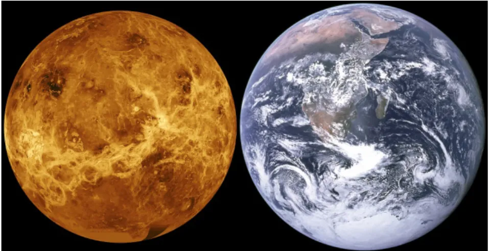
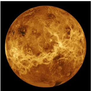
Shining visibly in the night sky, the second planet from the sun is a key piece to understand so many mysteries and answering the numerous questions that the universe can offer us. Also known as Earth’s twin, Venus (Fig. 1.1) is similar to our planet in radius, mass, density and overall bulk composition (Table 1.1) (Svedhem et al., 2007) . Both planets evolved from the same proto-solar nebula, and were formed (cooled down) at nearly the same time.

(16)

Figure 1.1: Venus and Earth sizes compared. Credit: NASA/JPL/Magellan

Earth Venus

Mass (kg) 5.98×1024 4.87×1024

Radius (km) 6378 6051

Density (g/cm3) 5.5 5.3

Distance to Sun (UA) 1 0.72

Sidereal Year (Earth days) 365 226 (0.26 year) Rotacional Period (Earth days) 1 243 (retrograde)

Obliquity (◦) 23.5 177

Solar Constant 1380 2610

Albedo 0.3 0.75

Equilibrium Temperature (◦C) -15 15

Surface Tempearture (◦C) 15 460

Surface Pressure (atm) 1 92

Atmospheric Composition 78.1% N₂ 20.9% O2 0.034% CO2 96% CO2 3% N2 Atmospheric Condensables H₂O H₂SO4

Table 1.1: Venus’ and Earth’s physical and atmospheric properties. Credit: Gon¸calves (2016)

However, if a closer look is taken at these “twins”, one can uncover the proof of the striking present contrasts between them. In spite of the existing solar system’s formation arguments that support the similar initial atmospheric conditions for both Venus and Earth, the two planets developed in fundamentally different ways. (Ringwood and Anderson, 1977) In the end, Venus presents us with conditions so different from Earth that we are left wondering how two planets could reach such contrasting states.

(17)

The motion of this planet is certainly one of the best examples of its peculiarities. Venus is the only terrestrial planet with a retrograde rotation in the whole Solar System. In addition, its obliquity, or axis tilt, is of 177◦, which means that Venus’ rotational axis is almost perpendicular to the ecliptic. Because of this, both of the planet’s hemispheres receive approximately the same amount of radiation throughout the year making seasonal variations negligible. (Bougher et al., 1997)

It is also worth mentioning that Venus is the slowest rotating planet of the Solar System. It takes about 243 Earth days (de Pater and Lissauer, 2007) to spin around (one day in Venus, 243 Earth days, is actually longer than a venusian year which is approximately 226 Earth days). If its retrograde rotation is considered, a solar day (the time it takes for Venus to rotate about its axis so that the Sun appears in the same position in the sky) is about 117 Earth days in total. (Grinspoon, 1997) It should also be expected that Venus’ atmosphere to keep up with this rotation speed, however the rotation of the solid planet contrasts dramatically with the much faster clouds’ rotation, which can circle Venus in only 4.4 days at 70 km of altitude and about 6 days at 48 km. This phenomena is widely known as superrotation and its driving mechanisms still lack a proper description and understanding. (Machado, 2013)

The surface conditions are also worthy of attention. For example, the extremely high pressure on the surface of Venus amounts to 90 times the atmospheric pressure on Earth’s surface, which is very close to 1 km depth at a terrestrial ocean. Furthermore, the 460◦C (730K) temperatures caused by the high CO2 concentration in the atmosphere and consequent runaway greenhouse effect mean that lead can melt on Venus’ surface. These aggressive conditions turn Venus’ surface into a hostile environment with a visual horizon that does not extend beyond 400 meters in a yellowish desolated world (probably due to sulphur compounds). (Grinspoon and Bullock, 2007) For Venus, thermodynamically speaking, the pressure and temperature at surface lead the atmospheric properties to be much closer to the liquid phase than a gaseous one.

1.2.1 Magnetic Field and Magnetosphere

Most planets and comets explored to date are encased in a strong magnetic field or magne-tosphere. These magnetic fields protect a planet from the charged particles streaming out from the Sun in the form of the solar wind that flows radially outward from the Sun at supersonic speeds, acting as a protective shield around the planet.

Venus is a rarity among planets. It is a world that does not internally generate a magnetic field. In part because of its slow rotation and its predicted lack of internal thermal convection, any liquid metallic portion of its core could not be rotating fast enough to generate a measurable global magnetic field (Russell, 2001).

This absence of an internal magnetic field and of a relevant magnetosphere leads to a direct interaction of the solar wind with the upper atmosphere, affecting the distribution of plasma particles and atoms in the excited state. Although, the evidence of a weak magnetic field around the planet suggests the hypothesis of a magnetosphere generated, not by a dynamo effect, as on Earth, but rather by the interaction of solar wind with the charged particles of the ionosphere (Goody and Walker, 1975). This is known as induced magnetic field or magnetosphere. Venus, Mars and Titan are examples of induced magnetospheres (Russell, 2001). Venus’ magnetosphere is far weaker than Earth’s and closer to the planet (Fig. 1.2).

(18)

Figure 1.2: Bow shock of the interaction between the plasma particles of solar wind and the induced Venus’ magnetosphere (upper part) and Earth’s intrinsic magnetosphere (lower part). Credit: Titov, D., in ”Planetary Atmospheres”

1.2.2 Geological Structure and Vulcanism

The fact that the density of Venus and Earth is so similar suggests that both these planets had a similar thermal history controlled by core differentiation. Since the two are approximately the same size and formed from similar primordial materials it is assumed that, in the beginning of planetary history (about 4.5 billion years), they had equal amounts of radioactive materials and consequently, produced roughly equal amounts of internal heat (Machado, 2013). Most thermal models suggest that Venus was initially mostly composed by chondritic (non-metallic) material. Its core might have accumulated most of it radioactive reservoir leading to a gradual rise of the planet’s temperature over time. Some of this internal heat escapes through molten crust rocks at hot spots. (Phillips and Malin, 1983) On Venus, these hot spots are not randomly scattered but rather concentrated in defined areas which are believed to be mantle plumes (Smrekar et al., 2010).

Venus’ internal structure is very much alike Earth’s and is composed by a thin silicate crust, a thick mantle and a heavy metallic core (nickel and iron). The major difference is that Venus’

(19)

core shows evidence of being solid and much colder than Earth’s. (Lewis, 2004) Although Venus does not show sign of active tectonic plates as on Earth, there are evident remains of deep gorges and canyons which can lead to a possibility of significant tectonic activity in the past (Machado, 2013). In Earth’s case, the plate tectonics mechanism is closely linked to the carbon dioxide cycle, burying large amounts of it at subduction zones, stabilising in this way the atmospheric amount of CO₂. Such process could not occur in the single plate Venus’ crust.

Figure 1.3: The hemispheric view of Venus, as revealed by more than a decade of radar investigations culminating in the 1990-1994 Magellan mission, is centered at 180 degrees east longitude. Credit: NASA/JPL/USGS

Venus’ surface is coated with volcanoes, lava flows and signs of impact craters. The low density of impact craters randomly scattered and almost pristine condition of the surface point to an age of 600-1100 million years (Schaber et al., 1992) and strongly suggests that an older surface was swept away and submerged by a large scale resurfacing process. A cataclysmic event capable of this would entirely disrupt the crust and consequently release a large amount of volatile components into the atmosphere. These impact craters found on Venus’ surface are generally quite large, since the thick atmosphere protects the planet against most impacts of smaller objects.

Regarding vulcanism, Venus does not have a thermal escape valve working in continuous mode as it happens on Earth, and consequently, the energy is accumulated and warms up the entire surface until lava erupts through thousands of volcanoes of all sizes. Periodically (on a scale of billions of years) the planet endures successive eras of intense vulcanism across the surface, erasing old craters and transfiguring the planet’s surface in enormous resurface processes. The past massive vulcanism and resurfacing episodes led to vulcanic outgassing of sulphur dioxide and water which was responsible for the formation of extensive sulphuric acid and water clouds, and the increasing albedo contributed to a cooling of the surface. Afterwards, a cloud differentiation process might have happened, which sank the heavier sulphuric acid droplets. The remaining thin high water vapour cloud layer endured photolysis under the upper atmosphere intense solar radiation, which caused the loss of atmospheric water. (Machado, 2013)

1.2.3 Runaway Greenhouse Effect

Despite having a solar constant of almost twice the Earth constant, Venus absorbs much less sunlight than our planet mainly due to the highly reflective cloud layer which completely envelops it, leading to an extremely high albedo of roughly 75%. This is one of the reasons that

(20)

Venus shines so brightly in the sky (reaching the apparent magnitude of −4.6), the brightest after the Sun and the Moon.

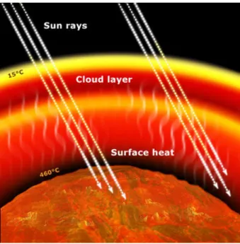
Figure 1.4: Schematic of Venus’ Runaway Greenhouse Effect. Credit: ESA website

If we consider Venus as a black body and also take into account its albedo, Venus would be cooler than Earth. So it appears that the major contribution for the high surface temperature in Venus is its atmosphere. By Wien’s displacement law (Eq. 1.1) the maximum of the wavelength radiation emitted (approximating Venus to a blackbody) is in the infrared range. The high concentration of CO₂ traps this planet’s infrared radiation causing it to be reabsorbed which leads to an uncontrolled greenhouse effect (Fig. 1.4), causing Venus to have the highest surface temperature among the planets of the solar system.

λmaxT = 2.898 × 10−3mK (1.1)

It is still unknown if the surface temperature has ever been low enough to allow condensation of water, even in possibly reduced solar illumination conditions in the early solar system which is a crucial question to answer regarding the complex evolution of the planet. (Chassefi`ere et al., 2012)

1.2.4 Venus’ Atmosphere Origin

It was during the formation of the solar system that planetesimals, orbiting in primitive orbit paths, swept through space collecting debris, dust and later gas, in a process denominated accretion. During this process there was a gravitational energy release, which added to the energy that comes from unstable radioactive isotopes. After this, because of the protoplanet rotation, which acts as a huge centrifuge, the planet suffers an internal differentiation process in layers (mantle and crust) depending on its constituents density. (Turcotte, 1995) It is during this phase that volatiles start to migrate to the surface where they can remain in liquid form

(21)

(like the oceans on Earth) or in gaseous form, which provides the planet with its own gaseous layer called atmosphere. There are other processes that can contribute to the formation of the atmosphere or its alteration (Fig. 1.5) but in short, the genesis of Venus’ atmosphere was, most likely, a process of accretion followed by a continuous degassing of volatiles from an intense mantle outgassing, as well, amplified by the overheating due to core differentiation processes. (Bullock and Grinspoon, 2001)

Atmosphere Alteration Processes

Processes by which the atmosphere gains gas: • Outgassing; • Cometary bombardment; • Accretion of planetesimals; • Evaporation/sublimation of deposited materials.

Processes by which the atmosphere loses gas:

• Thermal escape; • Chemical reactions; • Atmospheric impacts;

• Condensation onto the surface or clouds;

• Ionized particles bombardment.

Figure 1.5: Processes of atmospheric gain and loss of gases.

Composition

The telluric planets Venus, Earth and Mars had possibly similar atmospheres regarding primordial composition and relative abundances of its constituents. It was the evolutionary path that each planet followed that lead to extreme environments such as Mars and Venus or, in Earth’s case, a state where the existence of liquid water and life is possible. For example, although Earth’s and Venus’ atmospheres had roughly the same amount of carbon dioxide (CO₂), on Earth the major part of it is located in the crust (in the form of carbonated rocks) or dissolved in the vast oceans’ water. As for Venus, most of the carbon dioxide is present in the atmosphere leading to a massive greenhouse effect (Section 1.2.3). This makes Venus an interesting case to study the possible consequences of anthropogenic emissions of greenhouse gases and consequent climate changes on Earth.

The components of Venus’ atmosphere are in equilibrium with the rocks that cover the planet’s surface. Examples of these surface-atmosphere interactions include outgassing of vol-canic sulphur into the Venusian atmosphere and/or CO₂ absorption by the oceans on Earth. The analysis of the chemical reactions that affect atmospheric gases reveals that the chemical composition of Venus’ atmosphere is determined by surface properties. On Earth this is not the case. The reason for this different behaviour lies in two factors: On the one hand, desta-bilising processes such as photosynthesis perturbs CO2 levels affecting its concentration in the atmosphere. In the other hand, Venus’ surface temperatures lead to fast chemical reactions and consequently chemical equilibrium is reached quickly. (Machado, 2013)

Venus’ atmosphere is dominated by CO2 (Fig. 1.6) at the present stage of atmospheric evolution. However, it is the sulphur dioxide (SO₂) concentration along other minor components

(22)

Figure 1.6: Schematic of Venus atmosphere relative composition. Minor species relative abundances are given in the magnified portion of the left graph at the right side.. Credit: NASA website

that fine tunes its atmospheric balance. (Bullock and Grinspoon, 2001) This is one of the minor components of most importance regarding surface coupling. Also worth noting as a minor component is the carbon monoxide (CO) which is produced in the upper atmosphere due to the photolysis of CO2. In addition, it was also found evidence of the existence of H2O in the upper atmosphere, but only at trace level. (Beatty et al., 1999)

Venus loses its atmospheric CO₂ by photolysis in the upper part of the atmosphere, H₂O

is also lost by photolysis and by chemically reacting with SO₂ by forming sulphuric acid. Due to these losses, and to keep the dynamic atmospheric balance, it is necessary to have a source of replenishment.(Bullock and Grinspoon, 2001) Volcanic activity is the candidate for the re-plenishment process and abundance variability through time by injecting large amounts of these molecules during episodes of large-scale vulcanism.

Species Venus Earth Climate Significance

Carbon dioxide 0.96 0.0003 Major greenhouse gas

Nitrogen 0.035 0.770 Similar total amounts

Argon 0.00007 0.0093 Evolutionary clues

Neon 0.000005 0.000018 Evolutionary clues

Water Vapour 0.000030 ∼0.01 Volcanic, cloud, greenhouse Sulphur Dioxide 0.00015 0.2 ppb Volcanic, cloud, greenhouse Carbonyl Sulphide 0.000004 Volcanic, cloud, greenhouse Carbon Monoxide 0.00004 0.00000012 Deep circulation

Atomic Oxygen trace trace High circulation, escape processes Hydroxyl trace trace High circulation, escape processes

Atomic Hydrogen trace trace Escape processes

Table 1.2: Composition of the atmospheres of Venus and Earth as fractional abundances (percentages) except where parts per billion is stated (all except the noble gases argon and neon are observed by Venus Express instruments). (Credit: Taylor and Grinspoon, 2009)

(23)

Structure

The vertical stratification of the atmosphere is dictated by how gravity and pressure balance each other, represented in the hydrostatic equilibrium equation (Eq. 1.2)

dP

dz = −g(z)ρ(z) (1.2)

Here P represents the air pressure, z represents the altitude relative to the planet’s surface,

g(z) the gravitational acceleration and ρ(z) the density. (de Pater and Lissauer, 2007)

Since Venus is a planet which atmosphere is in equilibrium, its equation of state can be approximated by the ideal gas law (alternatively referred to as the perfect gas law):

P = N kT =ρRgasT µa

= ρkT

µamau

(1.3) Where N is the particle number density, µa the mean molecular weight(in atomic mass

units), Rgas is the universal gas constant and mau≈ 1.67 × 10−24 is the mass of an atomic

weight unit (slightly less than the mass of an hydrogen atom). (de Pater and Lissauer, 2007) Using both of the previous equations (1.2 and 1.3) one can find the equation to express pressure as function of altitude. Being H(r) the scale height:

P (z) = P0e−

Rz

0 dr/H(r) (1.4)

The variation of temperature with altitude divides Venus’ atmosphere into three distinct layers:

• Troposphere (0-65km): the densest part of Venus’ atmosphere which extends from the surface to the top of the clouds and where the temperature decreases with altitude with the thermal gradient ratio of about 9K · km−1 which is close to the adiabatic lapse rate (Γ_d=_Cq

p = 7.39 K · km

−1 _{). This shows that convection is not significant in this region;}

• Mesosphere (65-100km): characterised by a less pronounced vertical thermal gradient (Γ =∂T_∂Z) (Ahrens, 2003), being noticeable the relevant horizontal variability with latitude, increasing from the equator to the poles, which is consistent with the existence of a Hadley circulation cell (Taylor et al., 1980);

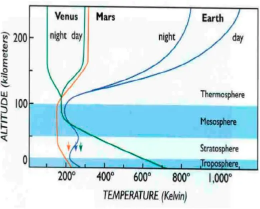
• Termosphere (100-200km): where the balance between the incident UV radiation and the thermal conductivity of the present molecules prevails. Here exists an asymmetry between the day and night hemispheres, as the daytime temperature tends to increase with altitude between 100 and 140 km, while at night it tends to decrease along the same altitude range, above 140 km the temperatures, at both hemispheres, becomes isothermal (Fig. 1.7).

(24)

Figure 1.7: Vertical temperature profiles of Venus’ atmosphere (green) compared with Mars’s (red) and Earth’s (blue) thermal profiles. Venus’ and Earth’s profiles are represented for both day and night.(Credit: B.Jakovsky).

The cloud deck on Venus has a determining influence on the planet’s albedo, thermal struc-ture and energy balance since most of the unidentified UV absorber abundance is at cloud layer. (Gon¸calves, 2016) It is responsible for half of the total absorbed energy coming from solar ir-radiation which efficiency is increased by scattering (ir-radiation travels longer paths). This way, the cloud medium, extending from 40 mbar (cloud top) until 1 bar (cloud base), see Fig. 1.8, absorbs roughly 92% of the incident solar flux (that is not reflected back to space due to the highly reflective albedo) and only the remaining 8% will actually reach the surface.

The cloud layer that covers the planet consists mainly of H₂SO4 droplets and a few other aerosols of unknown composition. It ranges from 48 km to 70 km of altitude (with about 22km of thickness) with hazes starting from the 30 km bellow the cloud deck and reaching up to 90 km above it. (Esposito et al., 1983) It can be divided into three layers (Fig. 1.9) when considering the average size of their aerosol particles: (Knollenberg and Hunten, 1980)

• Upper Layer (57-68 km): with an averaged particle radius of 0.3 µm, and a total optical depth of 7 at 0.63 µm;

• Middle Layer (51-56 km): with a predominance of 1 to 1.4 µm particle sizes, with an optical depth of about 9, at the same 0.63 µm wavelength;

• Lower Layer (48-50 km): with an optical depth of nearly 10 (at 0.63 µm wavelength), majorly due to 3.65 µm sized particles.

(25)

Figure 1.8: Pressure versus temperature profiles for Venus and Earth (Credit: Taylor and Grinspoon, 2009).

Figure 1.9: Venus’ sulphuric acid cloud deck and hazes extension in altitude. Regarding the averaged aerosol particles size, the cloud deck can be divided in the three layers shown in this scheme. (Figure: Titov,D.,private communication).

Several polarimetric and spectroscopic observations point to a general composition ratio of 25% H2O and 75% H2SO4 in terms of cloud particles. The sulphuric acid in the cloud tops is synthesised from photolysis and recombination process of H₂O and SO2 that reacts with CO2

(26)

according to the following chain reaction:

CO2+ SO2+ hν → CO + SO3 (1.5)

SO3+ H2O → H2SO4 (1.6)

Dynamics

Venus’ many fascinating characteristics and peculiarities are the root of its interesting at-mosphere dynamics, which differ from those observed on Earth, even though the two planets share a few similarities. As already stated (Section 1.2), the solid globe of Venus completes a full rotation once every 243 Earth days (de Pater and Lissauer, 2007) whereas its cloud system rotates much faster. The upper cloud layer has a rotation period of 4.4 days and the lower cloud layer of about 6 days. The atmosphere dynamics in Venus are mainly driven by its low rotation rate and thermal heating.

Figure 1.10: Large-scale motion of planetary atmospheres are dominated by various types of circulation patterns according to latitude, altitude and local time (left side: Earth and right side: Venus).

Three wind velocity components can be defined, being them:

− Zonal Wind (u) the component measured along the latitudinal lines; − Meridional Wind (v) the component measured along the meridians; − Vertical Wind (w) the upwards component of the winds.

We can also distinguish three main circulations processes that define Venus’ atmosphere dynamics:

(27)

1. Super-rotational retrograde zonal wind (RZW): where wind flows at great speed in quasi laminar bands parallel to the equator. This is the most relevant atmospheric motion in the mesospheric circulation (between the altitudes of 60-100 km and stretching between mid-latitudes). The RZW is also accompanied by a Hadley-type meridional circulation from the equator to poles and both converge into a unique polar vortex circulation. On the superrotating zonal retrograde circulation, two main non-asymmetric large scale features are super-imposed: the four-day planetary wave at low and mid-latitudes and a polar vortex in both the polar regions.

2. Subsolar to anti-solar circulation (SS-AS): which transports the overheated air from highly isolated regions towards the night side radiation deficit area above the 120 km of altitude. The greater exposure to solar radiation and lower density are the ones which drive this characteristic motion that highlights the contrast between the night and day sides of Venus when considering temperature and density.

3. Meridional Circulation (Hadley Cell): Characterised by one Hadley cell in each hemi-sphere which is responsible for the transport of heat excess from low latitudes, poleward to cooler latitude regions. The Hadley circulation cell consists of rising air near the equator and submersion at the poles (two equator-pole cells), converging in a polar vortex cir-culation. The net upward transport of angular momentum by the Hadley cell is able to maintain an excess of angular momentum in the upper part of the atmosphere, balanced by planetary waves equatorward transport. However this Hadley cell circulation is yet to be clearly characterised observationally and remains as more of a theoretical construct needing quantitative support. (Gon¸calves, 2016)

Figure 1.11: Venus global atmospheric circulation.(Credit: Taylor and Grinspoon, 2009)

Still regarding the dynamical aspects of the atmosphere of Venus, polar vortex motions, superrotation and atmospheric gravity waves (Section 1.3) will also be addressed for the purposes of this work.

(28)

Polar Vortex

The polar vortex (Fig 1.12), observed on both poles, is a three dimensional feature that is highly variable interchanging between a monopole, a dipole and a triple pole shape that has also been observed to change rather quickly (Luz et al., 2011). The vortex eye rotates around the polar axis faster than the RZW of the mid latitudinal range already discussed above in this section. The south pole vortex, observed recently, shows a period of about 2.7 terrestrial days and an exceptional variability in terms of shape (Luz et al. (2011); Garate-Lopez et al. (2013)). This means that the vortex eye rotates even faster than the super-rotating zonal winds of the mid latitudes range. It still remains to establish a relationship between the superrotation of the atmosphere and this phenomena which is a question regarded as a major theme in current scientific research.

Figure 1.12: (VMC images of Venus south polar vortex (left); Hurricane Frances on Earth (right). (Limaye et al., 2009)

Superrotation of Venus Atmosphere

There are still many open questions concerning the understanding of Venus’ atmospheric dynamics. One of them is how the superrotation process on Venus’ atmosphere is driven and how is it maintained over time.

This rotation of Venus’ atmosphere is not uniform, but depends on the latitude, a fact that can be seen by the relative motion of the cloud top layer, filleting the planet (Machado, 2013). The superrotation extends from the surface up to the cloud top ( ≈ 70 km altitude) with wind speeds of only few meters per second near the surface and reaching a maximum value of ≈ 100ms−1at the cloud top, corresponding to a rotation period of 4 Earth days ( ≈ 60 times faster than Venus itself) (Piccialli, 2010). It is indeed curious how an atmosphere of such a slow-rotating planet can be accelerated to such high speeds. Previous studies (Baker and Leovy (1987), Newman and Leovy (1992)) suggest that the superrotation is maintained by the transport of retrograde zonal momentum upward through thermal tides

(29)

at the equator and then poleward by a meridional cell. However, the attempts to model the zonal superrotation have only been partially successful so far which indicates that the mechanisms of this phenomenon are still unclear (Piccialli, 2010).

1.2.5 Venus Exploration

Many missions have departed from Earth, hoping to reach our neighbouring planet no more than a shining beacon in the sky with the name of a Goddess. Not all of them succeeded, but those which did have certainly returned a profound knowledge that still shapes our perception and understanding of space and the cosmos every single day. From the beginning of the space age, more than 30 different spacecrafts have been launched towards Venus making it the first successful planetary target for human space exploration with Mariner 2 in 1962.

The first attempts to reach Venus through robotic probes were made by the USSR. On February 1961, Tyazhely Sputnik and Venera 1 were launched, but both resulted in failures. It was only on the last month of the following year that Mariner 2 (NASA) made the first successful flyby to planet revealing that it was completely shrouded in an opaque atmosphere hiding the planet’s surface and deepening the mysteries it offered.

Venera Missions (1961-1984)

The Venera program collected the first images from the surface (Fig. 1.13) and gathered information about surface chemical and physical conditions. The mission had its beginning in 1961 but suffered some initial failures and its success only became apparent later with Venera 4 that collected and sent back to Earth the first atmospheric data in 1967. A few of the Venera probes successfully landed and survived long enough on the surface in order to transmit back to Earth the data they collected. Among many scientific contributions, the Venera missions produced high resolution radar surface mapping and confirmed the existence of the superrotation phenomenon on Venus’ atmosphere (Dollfus, 1975).

Mariner Program (1962-1973)

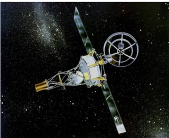
The Mariner program consisted of ten exploration probes designed by NASA which main aim was to investigate the planets. Mariner 1, 2, 5 and 10 were sent to Venus and Mariner 2 (Fig. 1.14) was the first probe to reach close contact (due to launch issues Mariner 1 ended up failing). The measurements made with its magnetometer confirmed the high surface temperatures of 460◦C (Sonett, 1963).

(30)

Figure 1.13: Surface images of Venus, taken from the Venera landers which were among the first images taken by mankind inside another planet. Credit:Hamilton (2005)

(31)

Figure 1.14: Mariner 2. Credit: NASA/JPL

Pioneer Mission (1978-1992)

The Pioneer Venus mission (NASA) consisted of two components launched separately: a Multiprobe and an Orbiter both launched in 1978. Due to its high elliptical orbit, the Pioneer allowed a global mapping of the cloud deck, ionosphere, upper atmosphere, surface mapping by radar, among many other experiments and contributions. The performed measurements of cloud and atmospheric properties were essential in the development of Venus atmospheric models (Collin and Hunten, 1977).

The mission was also the one responsible for the first measurements of Venus’ weak magnetic field by means of an on-board magnetometer which was later confirmed by ESA’s Venus Express. Another achievement was the discovery of the vast double vortex at the northern polar region of Venus.

On 1992, after running out of fuel, the Pioneer Mission came to its conclusion.

Vega (1984-1985)

As a continuation of the previous Venera program, this spacecraft mission combined a Comet Halley flyby and a Venus swingby and two identical spacecrafts, Vega 1 and Vega 2, were launched on December 1984 only a few days apart. The mission now included atmospheric balloons, besides the same basic probes and landers designs, as these could survive longer and measure the temperature, pressure and wind velocity (Blamont, 2008). The Vega and Pioneer missions were essential for the structured study of the atmospheric physical description and chemical behaviour since their measurements uncovered evidence of an active atmosphere, containing corrosive gases and also a thick cloud layer.

Magellan (1989-1994)

Named after the sixteenth-century Portuguese explorer Fern˜ao de Magalh˜aes, the Magellan spacecraft from NASA was launched on May 1989 and arrived at its destiny on August 1990. Magellan collected radar images of Venus’ surface with resolution ten times better than the earlier Soviet Venera 15 and 16 missions (around 200 meters). The surface topography and electrical characteristics were also measured using radiometry and altimetry data. Upon reaching

(32)

the end of its already extended mission, the probe was crashed into the planet in a controlled manner with the last aim of obtaining some atmospheric data along its descent (Saunders et al., 1992).

Figure 1.15: Venus’s surface obtained through radar data from the Magellan Orbiter in 1992. Credit: NASA/JPL. Magellan Project

Galileo (1989-2003)

On its way to Jupiter, the Galileo spacecraft made a Venus fly-by gravity assisted maneuver and made a few observations during its closest approach, taking advantage of Galileo’s high resolution infrared camera. The images taken contributed to deepen the knowledge about cloud properties and their variability (Carlson et al., 1993). Galileo ceased operations on September 2003 after observing Venus, the Moon, Jupiter, two asteroids (Gaspa and Ida) and the comet Shoemaker-Levy 9 fragments from the impact with Jupiter.

Venus Express (2005-2015)

Venus Express (VEx) (Fig. 1.16) wass a spacecraft lauched by the European Space Agency (ESA) on the 9thof November of 2005. Its main objective was to perform a global investigation of the venusian atmosphere breaking the long period without any space missions sent to this planet. Vex arrived at Venus on April 2006 and conducted studies under the general atmo-spheric circulation, cloud chemistry and escape processes for several distinct volatiles as well as interactions/connections between the surface and the atmosphere.

(33)

Figure 1.16: ESA’s Venus Express, being packed ready to leave INTESPACE, Toulouse, for its launch site in Baikonur, Kazakhstan. It is shown with high-gain antenna wrapped and solar arrays folded. Credit: ESA

The orbital design was elliptical and highly eccentric (250 km at pericenter and 66 000 km at apocenter), with a period of 24 hours. This allowed global large scale investigations and high spatial resolution detailed studies of localised phenomena. After years of gathering knowledge and providing amazing discoveries, VEx’s remaing fuel was exhausted and the contact with the spacecraft was lost. The mission reached its official end upon a declaration by ESA on the 16th of December of 2014.

Venus Express most relevant scientific discoveries included the possibility of recent vulcanism, the atmosphere’s superrotation speeding up, Venus’ spinning slowing down, confirmation of the existence of a magnetosphere, the shape-shifting polar vortices and that Venus is loosing water through escape processes.

ESA’s spacecraft carried on board some of the cutting-edge technology instruments at the time which included (Fig. 1.21):

Figure 1.17: A cutaway diagram showing size and locations of Venus Express instruments: MAG, VIRTIS, PFS, SPICAM/SOIR, VMC, VeRa and ASPERA. Credit: ESA

(34)

• ASPERA (Analyser of Space Plasma and Energetic Atoms): designed to study the interaction between the venusian atmosphere and the solar wind, measuring outflowing particles from Venus’ atmosphere and the ones that make up the solar wind and investi-gating how ions and molecules escape the planet;

• PFS (Planetary Fourier Spectometer): a high resolution instrument that measured the atmosphere’s temperature from 55 km to 100 km of altitude as well as the surface’s temperature, looked for vulcanic activity and made some composition measurements of the atmosphere;

• VeRa (Venus Radio Science Experiment): used the radio link between itself and Earth to investigate Venus’ ionosphere. In addition, it was used to study the atmosphere’s pressure, temperature and density (35 km up to 100 km of altitude) as well as electrical properties of the surface.

• MAG (Venus Express Magnetometer): studied the magnetic field generarted by the interaction between the atmosphere and the solar wind and its contribution to atmospheric escape processes;

• SPICAV/SOIR (Ultraviolet and Infrared Atmospheric Spectometer): searched for water in Venus’ atmosphere and helped in determining the density and tempearture between 80 km and 180 km of altitude;

• VMC (Venus Monitoring Camera): is a wide-angle multi-channel camera capable of taking images of the planet in near-infrared, ultraviolet and visible wavelengths. It was able to make global images and study the cloud dynamics as well as imaging the surface.

Figure 1.18: VMC filter parameters. Credit: ESA

• VIRTIS (Ultraviolet/Visible/Near-Infrared Mapping Spectometer): was an imag-ing spectrometer that combined three observimag-ing channels in a simag-ingle but powerful instru-ment. Its data can be used for cloud tracking (Section 2.5) in both infrared and ultraviolet wavelengths allowing the study of atmospheric dynamics at different altitudes.

(35)

Figure 1.19: Summary of VIRTIS characteristics. Credit: ESA website

Akatsuki or Venus Climate Orbiter

Akatsuki, meaning Dawn or Venus Climate Orbiter (VCO) is a Japanese (JAXA) space probe launched on 20 May 2010, but failed to enter orbit around Venus on 6 December 2010. After the craft orbited the Sun for five years, engineers successfully placed it into an alternative Venusian elliptic orbit on 7 December 2015 and Akatsuki could then begin its mission and it is still operational. Akatsuki’s current orbital path takes it as close as 400 km to Venus,and as far away as 44 0000 km and has aperiod of 10.8 days. The goal of the Akatsuki project is to clarify the three dimensional motion of Venusian atmosphere over time and establish a meteorology of Venus. In order to achieve the ambitious goal, Akatsuki was equipped with several instruments introduce bellow:

• LAC (Lightning and Airglow Camera): is a camera which can detect lightning dis-charge at small intervals wich can be used to solve the controversial topic of lightning occurrence in the venusian atmosphere. In addition to this, it captures airglow produced by oxygen in the higher atmosphere allowing the visualisation of atmospheric waves and circulation between nightside and dayside;

• IR1 (1 µm Camera): uses the bands around 1µm allowing the observation bellow the clouds and near the surface of the planet. It can also allow, by comparing different infrared bands, to investigate the cloud movement in the lower atmosphere, the distribution of water vapor, the surface’s mineral composition and look for the presence of volcanoes;

• IR2 (1 µm Camera): is used to observe the density and size of the cloud particles since the 2µm wavelengt is emmited from bellow the bottom of Venus’ clouds. This will make possible to gain insight into atmospheric circulation at lower altitudes and into the formation process of clouds.

• LIR (Long-wave infrared camera): uses the 10µm wavelength to measure the temper-ature at the cloud tops making possible to study convection within the upper cloud layer as well as wind speed distributions on the upper cloud tops of both dayside and nightside; • USO (Ultra-Stable Oscillator): When Akatsuki is concealed behind Venus as seen from the Earth, the radio waves transmitted by the USO graze the venusian atmosphere,

(36)

Figure 1.20: Akatsuki’s components and main instruments. Credit: JAXA

changing their frequency, and reach the Earth. Analysing those changes allows scientists to measure the vertical profiles of temperature and sulphuric acid vapour;

• UVI (Ultraviolet Imager): acquires ultraviolet images, allowing us to obtain the dis-tribution of sulphur dioxide, which is related to the cloud formation, and the disdis-tribution of unidentified chemical substances which absorbs the ultraviolet rays. Also, wind speeds at the cloud tops can be determined by tracing the dark-and-light pattern due to the scattering of ultraviolet rays in sunlight by Venusian clouds. This instrument operates in two different wavelengths:

1. Ultraviolet - 283 nm (dayside of Venus and targets sulphur dioxide at cloud top); 2. Ultraviolet - 365 nm (dayside of Venus and targets the unidentified absorbent

(37)

(38)

1.3 Atmospheric Gravity Waves

Atmospheric gravity waves play an essential role in the global circulation of a planet’s atmo-sphere. Generally observed in the stratosphere of most planets with atmosphere, these waves are periodic disturbances whose restoration force is buoyancy (Piccialli et al., 2014). They are responsible for very important dynamic phenomena such as, for example the vertical transfer of energy, momentum and chemical species (atmospheric gravity waves transport energy and momentum from the troposphere and deposit it in the thermosphere and mesosphere) and it is through its properties that one can draw conclusions about the static equilibrium of the at-mosphere since these waves can only propagate in stably stratified regions of the atat-mosphere (Nappo, 2012). On Venus, gravity waves at cloud level might be due to convective motions of a lower unstable layer beneath the stable layer where these waves form. In addition, they could also be excited by Kevin-Helmholtz instabilities produced by a strongly sheared flow when close to neutral static stability (S´anchez-Lavega, 2011).

On Earth, atmospheric gravity waves are frequently generated in the troposphere by the clash of two different weather fronts or by airflow over mountains. These waves have a tendency to propagate to higher altitudes where they suffer the influence of nonlinear effects and break, transferring the energy and momentum that they carry to the mean flow of the atmosphere (S´anchez-Lavega, 2011).

Figure 1.22: Atmospheric gravity waves on Earth’s atmosphere over the Arabian Sea. Credit: NASA

A recent study (Piccialli et al., 2014) involving high resolution images acquired by Venus Monitoring Camera (VMC), at the cloud tops at high latitudes in the Northern hemisphere, observed periodic structures that have been interpreted as atmospheric gravity waves. Wave properties do not seem to vary with local time or latitude but this information is biased since VMC could not observe latitudes lower than ≈ 45◦S and neither with enough resolution (to

observe these features clearly) on the nightside, considering the observations period in the pub-lished paper (Piccialli et al., 2014). The most wave activity was found between 60◦N and 80◦N

(cold collar region) and was also concentrated above a continental highland in Venus (Piccialli et al., 2014).

(39)

Another systematic search for gravity waves was also carried out by (Peralta et al., 2008) but with the Visible and InfraRed Thermal Imaging Spectometer (VIRTIS) observations. Mesoscale gravity waves were detected in the upper cloud tops at about 66 km of altitude (using reflected ultraviolet light at 380 nm) on the dayside hemisphere and in the lower cloud layer at about 47 km of altitude (using 1.74µm thermal radiation) from the nightside hemisphere. The wave properties that were also measured included packet length, width, orientation and geographical position on Venus.

(40)

Chapter 2

Methods and Tools

2.1 Vex/VIRTIS-M

The VIRTIS imaging spectrometer is an instrument directly inherited from ESA’s Rosetta cometary mission. It is composed by two separate telescopes that supply two different channels: VIRTIS-M, which is a mapping spectrometer working in the infrared and visible wavelengths (Fig. 1.19) and VIRTIS-H, a high resolution spectrometer that operates in the Infrared. With its unique combination of mapping capabilities at low spectral resolution (VIRTIS-M) and high spectral resolution slit spectroscopy (VIRTIS-H), the instrument is ideal for making extensive infrared and visible spectral images of planet Venus (Piccioni et al., 2007).

VIRTIS-M has also a noteworthy capability of capturing images simultaneously at differ-ent wavelengths, compressing this information into a three dimensional structure called “data cube”. Using this we are provided with a vertical profile of Venus’ cloud structure at different wavelengths and we are capable of studying the cloud dynamics at different altitudes. VIRTIS data is gathered and stored in the Planetary Science Archive (PSA) of ESA, where it appears divided into three types: RAW, GEOMETRY and CALIBRATED.

- RAW: are the non-navigated VIRTIS images. These have only been subjected to prelimi-nary processing from telemetry data, which comes from the spacecraft, that is analysed by VEx’s ground segment tasked with writing the data files. These data files are then made available in ESA’s archive as Planetary Data System (PDS) files;

- GEOMETRY: is the data which comprises all the geometrical information of a specific image. It is basically the file that stores information on navigation measurements and geometrical calculations performed during calibration;

- CALIBRATED: are image files that have been processed. This means that these images are navigated and corrected in terms of instrument defects. The data in calibrated images is in physical units (radiance) and provides a description of viewing configurations (location, local time, viewing angles and season).

Regarding the contents of this work, the CALIBRATED data was the one used since it already possessed the geographical information of geometry data and is mostly corrected for defects present in RAW images. In short, the CALIBRATED images are the most suitable for both cloud tracking and gravity wave detection and characterisation.

(41)

2.2 Vex/VMC

The images captured through the VMC instrument on board Venus Express have allowed a complementary investigation of phenomena observed with VIRTIS. Despite this, VMC is better tuned for wavelengths in the visible light part of the spectrum, therefore, it was mostly used to analyse the upper clouds of Venus. In particular, UV-absorption of the top cloud layers produces noticeable features which can be tracked for wind velocity measurements. These absorptions are mainly due to the presence of sulphur dioxide and a still unidentified and unknown absorber (Markiewicz et al., 2007).

VMC images also allow search and visualisation of atmospheric mesoscale gravity waves (Section 1.3). The images with positive detections of these waves allow a certain degree of characterisation by measuring width, length, wavelength and altitude (Piccialli et al., 2014).

Unfortunately, the analysis of VMC images with PLIA (Section 2.4) was limited since the built-in navigation algorithm in PLIA was, at the time of study, not able to compute latitude-longitude coordinates for each of the image’s pixels. Nevertheless , some information can still be extracted, namely the time associated with each image as well as the date. For cloud tracking purposes (explained bellow in this chapter) this can be troublesome since image navigation is required for the image correlation software to function. As such, navigated images were provided through contact with Ricardo Hueso and Javier Peralta so that this study could be performed with several different instruments and a more in depth exploration of the software could be made.

2.3 Akatsuki/UVI

The UVI instrument carried by the still operational Akatsuki takes ultraviolet (UV) images of the solar radiation reflected by the Venusian clouds, with narrow bandpass filters centered at the 283 nm and 365 nm wavelengths. These wavelengths are considerably relevant since there are absorption bands of sulphur dioxide (SO2 which has an absorption band in the wavelengths 210–320 nm) and unknown absorber (which maximum absorption is around 400 nm) in these cloud regions (Pollack et al. (1980) and Esposito et al. (1997)). UVI takes nominal sequential images every 2 hours considering that higher observation frequencies are inhibited to maintain the thermal condition of the instrument.

The UV images are able to provide the spatial distribution of SO₂and the unknown absorber around cloud top altitudes. In addition, these images are used to estimate the horizontal winds by tracking cloud features. The images also allow a better understanding of the cloud top mor-phology and haze properties. UVI data, combined with data from other onboard instruments, is also used for the investigation of the generation mechanism of superrotation in the Venus’ atmosphere (Yamazaki et al., 2018).

(42)

Observation target Solar radiation scattered at cloud top Optics design Camera with off-axial catadioptric optics

Observational wavelength 283 and 365 nm

Field-of-view 12◦

FOV per pixel 0.20 mrads

Spatial resolution ∼200 m (periapsis)–76 km (60Rv)

Optics

F-number 16

Focal length 63.3 mm

Aperture size 39.89 mm (hood entrance)

Bandpass widths of the filters 14 nm

Detector

CCD SiCCD (back-illuminated and full-frame transfer)

Pixel number 1024 × 1024 pixels

CCD control

Exposure time 4 ms–11 s

Data depth 12 bit

Table 2.1: Characteristics of UVI from VCO where RV is Venus’ radius. Credit: Yamazaki et al. (2018)

2.4 PLIA - Planetary Laboratory Image Analysis

PLIA is an integrated set of programs written in Interactive Data Language (IDL) that possesses a fully operational and practical Graphic User Interface (GUI). PLIA was developed at the University of the Basque Country and was shared wit the research group in Lisbon by the Bilbao team in a shared study collaboration opportunity.

PLIA’s software aims to aid in the study of atmosphere dynamics by allowing the processing of astronomical images. This includes, to some extent, planetary navigation which is essentially the assignment of longitude and latitude values to each one of the pixels in an image. Such nav-igation is imperative and crucial to most of scientific measurements in planetary sciences since it becomes possible to ascertain the position, displacement and velocity of surface and atmo-spheric features present on planets and moons. PLIA also incorporates a wide range of numerous image correction tools, some dedicated to certain instruments like VEx/VIRTIS, photometric scans and is also capable to compute geometric projections of images into cylindrical and polar maps, which are useful for cloud-tracking procedures. These geometrical projections show only small sections of the complete Venus’ map, where the size is inherited from the original limits of the unprocessed image. This a crucial step for cloud tracking which is performed by auxiliary software to PLIA described in later sections.

One of PLIA’s most important and useful features is the possibility of performing image corrections, exemplified by Figure 2.1. Even on already calibrated data, this element is helpful for extracting features for our study. Most “original” images, untouched by the software, are not appropriate for the identification of more subtle features such as cloud formation hence some treatment is required before proceeding to the analysis. Additionally, images may contain artificial features of the detector that can be diminished and removed with the software when possible.