www.atmos-chem-phys.net/17/1847/2017/ doi:10.5194/acp-17-1847-2017
© Author(s) 2017. CC Attribution 3.0 License.
Effects of atmospheric dynamics and aerosols on the fraction of
supercooled water clouds
Jiming Li1, Qiaoyi Lv1, Min Zhang1, Tianhe Wang1, Kazuaki Kawamoto2, Siyu Chen1, and Beidou Zhang1
1Key Laboratory for Semi-Arid Climate Change of the Ministry of Education, College of Atmospheric Sciences,
Lanzhou University, Lanzhou, China
2Graduate School of Fisheries Science and Environmental Studies, Nagasaki University, Nagasaki, Japan Correspondence to:Jiming Li ([email protected])
Received: 16 February 2016 – Discussion started: 25 February 2016
Revised: 27 December 2016 – Accepted: 19 January 2017 – Published: 8 February 2017
Abstract. Based on 8 years of (January 2008– December 2015) cloud phase information from the GCM-Oriented Cloud-Aerosol Lidar and Infrared Pathfinder Satellite Observation (CALIPSO) Cloud Product (GOCCP), aerosol products from CALIPSO and meteorological pa-rameters from the ERA-Interim products, the present study investigates the effects of atmospheric dynamics on the supercooled liquid cloud fraction (SCF) during nighttime under different aerosol loadings at global scale to better understand the conditions of supercooled liquid water gradually transforming to ice phase.
Statistical results indicate that aerosols’ effect on nucle-ation cannot fully explain all SCF changes, especially in those regions where aerosols’ effect on nucleation is not a first-order influence (e.g., due to low ice nuclei aerosol fre-quency). By performing the temporal and spatial correla-tions between SCFs and different meteorological factors, this study presents specifically the relationship between SCF and different meteorological parameters under different aerosol loadings on a global scale. We find that the SCFs almost decrease with increasing of aerosol loading, and the SCF variation is closely related to the meteorological parameters but their temporal relationship is not stable and varies with the different regions, seasons and isotherm levels. Obviously negative temporal correlations between SCFs versus vertical velocity and relative humidity indicate that the higher vertical velocity and relative humidity the smaller SCFs. However, the patterns of temporal correlation for lower-tropospheric static stability, skin temperature and horizontal wind are rel-atively more complex than those of vertical velocity and hu-midity. For example, their close correlations are
predomi-nantly located in middle and high latitudes and vary with lat-itude or surface type. Although these statistical correlations have not been used to establish a certain causal relationship, our results may provide a unique point of view on the phase change of mixed-phase cloud and have potential implications for further improving the parameterization of the cloud phase and determining the climate feedbacks.
1 Introduction
Cloud feedbacks are recognized as the greatest source of un-certainty in the climate change predictions projected by cli-mate models (Boucher et al., 2013). One of the outstanding challenges to better understanding the role of clouds in fu-ture climate change involves how to more accurately deter-mine the cloud phase composition between 0 and −40◦C (Tsushima et al., 2006; McCoy et al., 2015; Tan et al., 2016). As we know, clouds are composed entirely of liquid or ice particles when temperatures are above the freezing (0◦C) or below homogeneous freezing (approximately −40◦C),
respectively (Pruppacher and Klett, 1997). Between 0 and −40◦C, clouds may consist of pure ice, liquid particles or
1848 J. Li et al.: Effects of dynamics and aerosols on the cold cloud phase
the total cloud radiative impact of mixed-phase clouds de-creases as supercooled clouds glaciate. In addition, the phase composition also has an important impact on the cloud pre-cipitation efficiency and lifetime (Pinto, 1998; Jiang et al., 2000).
Generally speaking, the changes of cloud phase compo-sition in mixed-phase clouds is complicatedly controlled by several factors other than temperature, e.g., ice nuclei (IN) (Choi et al., 2010; Tan et al., 2014; Zhang et al., 2015) or dynamical processes (Trembly et al., 1996; Shupe et al., 2008). Some special aerosols suspended in the atmosphere can change the cloud phase by acting as IN in the heteroge-neous ice nucleation process of mixed-phase clouds via dif-ferent nucleation modes (e.g., deposition, immersion freez-ing, contact and condensation freezing) (Lohmann and Fe-ichter, 2005). For example, based on laboratory experiments and field measurements, mineral dust from arid regions has been widely recognized as an important source of IN in mixed-phase clouds because of its nucleation efficiency and abundance in the atmosphere. In addition to dust, some stud-ies have also verified the potential ice nucleation ability of polluted dust and smoke at cold temperatures (Niedermeier et al., 2011; Cziczo et al., 2013; Tan et al., 2014; Zhang et al., 2015). For dynamical process, Naud et al. (2006) assessed the impact of large-scale ascent on the cloud phase and found that the areas of greatest large-scale ascent are not glaciated at cloud top as much as areas of moderate ascent. If large-or meso-scale models are unable to appropriately resolve these microphysical and dynamical processes, they will fail to accurately separate the cloud phase composition, which further affect the major climate feedbacks of global climate models by changing cloud, water vapor, lapse rate and sur-face albedo (Choi et al., 2014). For example, by conducting a multi-model intercomparison of cloud-water in five state-of-the-art atmospheric general circulation models (AGCMs), Tsushima et al. (2006) found that the difference in mixed-phase cloud algorithms among different models can result in different poleward redistribution of cloud liquid water, there-fore causing the difference in albedo feedback in the models. Those models which have less cloud ice in the mixed-phase layer will lead to higher climate sensitivity due to the posi-tive solar cloud feedback. It is therefore of fundamental im-portance to know the spatiotemporal distributions of different cloud phases, especially supercooled liquid clouds, and their variation with the IN or environmental conditions changing to improve the simulation of mixed-phase clouds in the cur-rent climate models and reduce uncertainties in-cloud feed-back within models.
Compared with the passive remote sensing (Huang et al., 2005, 2006a), the millimeter-wavelength cloud-profiling radar (CPR) on CloudSat (Stephens et al., 2002) and the Cloud-Aerosol Lidar with Orthogonal Polarization (CALIOP) (Winker et al., 2007) on Cloud-Aerosol Lidar and Infrared Pathfinder Satellite Observation (CALIPSO) can provide more detailed data regarding the vertical structure
of clouds, along with cloud phase information on a global scale (Hu et al., 2010; Li et al., 2010, 2015; Lv et al., 2015). The depolarization ratio and layer-integrated backscatter in-tensity measurements from CALIOP can help distinguish cloud phases (Hu et al., 2007, 2009). For example, by us-ing combined cloud phase information from CALIOP and temperature measurement from Imaging Infrared Radiome-ter (IIR), Hu et al. (2010) compiled the global statistics re-garding the occurrence, liquid water content and fraction of supercooled liquid clouds. Based on the vertically resolved observations of clouds and aerosols from CALIOP, Choi et al. (2010) and Tan et al. (2014) analyzed the variation of su-percooled water cloud fraction and possible dust aerosol im-pacts at given temperatures. For dynamic processes, although some studies have focused on the impacts of large-scale me-teorological parameters on supercooled water cloud fraction at regional scale based on observation (Naud et al., 2006) or global scale in observations and models (Cesana et al., 2015), related studies of the statistical relationship between cloud phase changes and meteorological parameters under different aerosol loadings have received far less attention. For the above reasons, this study combines cloud phase in-formation from the GCM-Oriented CALIPSO Cloud Product (GOCCP) (Chepfer et al., 2010), meteorological parameters from ERA-Interim reanalysis datasets and the aerosol prod-uct from CALIPSO to investigate the correlations between supercooled liquid cloud fraction (SCF) and meteorological parameters under different aerosol loadings at a global scale. This paper is organized as follows: a brief introduction to all datasets used in this study is given in Sect. 2. Section 3.1 outlines the global distributions and seasonal variations of SCFs and IN aerosol (here, dust, polluted dust and smoke). Further analyses regarding the temporal and spatial correla-tions between SCFs and meteorological parameters are pro-vided in Sects. 3.2 and 3.3. Important conclusions and dis-cussions are presented in Sect. 4.
2 Datasets and methods
In the current study, 8 years (January 2008–December 2015) of data from CALIPSO-GOCCP, the ERA-Interim daily product (Dee et al., 2011) and the CALIPSO level 2 5 km aerosol layer product are collected to analyze the effects of meteorological parameters on the SCFs under different aerosol loadings at a global scale.
2.1 Cloud phase product
backscatter and radar reflectivity to distinguish ice clouds, typical mixed-phase clouds, where a liquid top overlies the ice, and liquid clouds. However, the lidar-only method dis-criminates cloud phase based on the following physical basis. That is, nonspherical particles (e.g., ice crystal) can change the state of polarization of the laser light backscattered and result in large values of the cross-polarization component (ATB⊥)of attenuated backscattered signal (ATB), whereas spherical particles (e.g., liquid droplets) do not if the effects of multiple scattering are neglected.
As a lidar-only cloud climatology, the main goal of CALIPSO-GOCCP climatology is to facilitate the evalua-tion of clouds in climate models (e.g., Cesana and Chepfer, 2012; Cesana et al., 2015) with the joint use of the CALIPSO simulator (Chepfer et al., 2008). Thus, GOCCP has been de-signed to diagnose cloud properties from CALIPSO observa-tions in same way (e.g., similar spatial resolution, same cri-teria for cloud detection and statistical cloud diagnostics) as in the CALIPSO simulator included in the Cloud Feedback Model Intercomparison Project (CFMIP, http://www.cfmip. net) Observation Simulator Package (COSP) used within version 2 of the CFMIP (CFMIP-2) experiment (Bodas-Salcedo et al., 2011). This ensures the differences of the observations and the “model+simulator” ensemble outputs are mostly attributed to model biases (e.g., Cesana et al., 2012; Cesana and Chepfer, 2012). The CALIPSO-GOCCP cloud algorithm includes following steps. First, the instan-taneous profile of the lidar attenuated scattering ratio (SR) at a vertical resolution of 480 m is generated from ev-ery CALIPSO level 1 lidar profile (horizontal resolution of 333 m). Here, SR is the ratio of the total ATB to the com-puted molecular attenuated backscattered signal (ATBmol,
only molecules). Then, each atmospheric layer is labeled as cloudy (SR≥5 and ATB–ATBmol> 2.5×10⁻³km−1sr−1),
clear (0.01≤SR < 1.2), fully attenuated (SR < 0.01) or uncer-tain pixel (1.2≤SR < 5) to construct the three-dimensional cloud fraction. However, it is worth noting that a threshold of 5 for SR in CALIPSO-GOCCP cloud algorithm may miss some subvisible clouds (optical depth < 0.03) and result in the underestimation of optical thin cloud layers (e.g., Chep-fer et al., 2013). Some dense dust or smoke layers also can be misclassified as cloudy pixels (Chepfer et al., 2010). For every cloudy pixel, CALIPSO-GOCCP product further clas-sifies as “ice”, “liquid” or “undefined” sample by using the 2-D histograms of ATB, ATB⊥ and a phase discrimination line (Cesana and Chepfer , 2013). Those “undefined” sam-ples include three ambiguous parts: (1) cloudy pixels located at lower altitudes than a cloudy pixel with SR > 30, (2) cloudy pixels with abnormal value of depolarization (e.g., ATB⊥< 0 or ATB⊥/(ATB–ATB⊥)> 1) and (3) horizontally oriented ice particles. Cesana and Chepfer (2013) indicated that these “undefined” samples account for about 10.3 % of cloudy pix-els in 15 months of global statistics. In addition, because li-dar cannot penetrate optically thick clouds (optical depth > 3, such as the supercooled liquid layer in the polar region) to
de-tect ice crystals (Zhang et al., 2010), the CALIPSO-GOCCP cloud phase products possibly lead to a slight underestima-tion of ice clouds at the lowest levels at Arctic (Cesana et al., 2016).
In the present analysis, the cloud phase infor-mation during nighttime is derived from the 3-D_CloudFraction_Phase_temp monthly average dataset in the CALIPSO-GOCCP v2.9 cloud product. This dataset includes cloud fractions for all clouds (“cltemp”), liquid (“cltemp_liq”), ice clouds (“cltemp_ice”) and undefined clouds (“cltemp_un”) as a function of the temperature in each longitude–latitude grid box (2◦×2◦). In addi-tion, the temperature used here is obtained from GMAO (Global Modeling and Assimilation Office; Bey et al., 2001), which is part of the CALIPSO level 1 ancillary data. For each CALIOP level 1 profile, the GMAO tem-perature is interpolated over the 480 m vertical levels of CALIPSO-GOCCP as the cloudy pixel temperature. That is, the temperature bins are ranged every 3◦C and 38 temperature bins are provided for each parameter. Those liquid phase clouds whose high bounds of temperature bins are lower than 0◦C are considered as supercooled water phase clouds. Similar to the definition of SCF from Choi et al. (2010) and Tan et al. (2014), we calculate the SCF at a given temperature bin (or isotherm) as the ratio of the
cltemp_liq/(cltemp_liq+cltemp_ice) in a 2◦×2◦ grid box. Because there are no−10,−20 and−30◦C isotherms in the CALIPSO-GOCCP product, the present study uti-lizes the 22nd (from−27 to −30◦C), 25th (from −18 to −21◦C) and 28th (from −9 to −12◦C) temperature bins
to represent−30,−20 and−10◦C isotherms, respectively.
Choi et al. (2010) has pointed out that this definition may lead to some overestimation of SCFs without considering horizontally oriented ice particles, which account for about 10 % of the uncertainty in their study. However, the impact of the oriented ice crystals on the determination of cloud phase is negligible after tilting the CALIOP to 3◦off-nadir (November 2007) (Hu et al., 2009; Cesana et al., 2016). 2.2 Meteorological reanalysis dataset
Hart-1850 J. Li et al.: Effects of dynamics and aerosols on the cold cloud phase
Figure 1.The global and seasonal variations of supercooled water cloud fractions (SCFs) and relative aerosol frequencies (RAFs) during nighttime at−10◦C isotherm over 2◦×2◦grid boxes.
mann, 1993), as described below:
1θ=T700
1000 p700
R/Cp −Tsfc
1000 psfc
R/Cp
, (1)
whereppresents pressure,T is temperature andR andCp denote the gas constant of air and the specific heat capacity at a constant pressure, respectively. Note that a high LTSS value represents a stable atmosphere and the positive vertical velocity implies updraft in this study, and vice versa. In ad-dition, it needs further noting that the vertical velocity used in this investigation is referred to the large-scale vertical mo-tion and is different from the in-cloud updrafts velocity men-tioned in previous studies (Rauber and Tokay, 1991; Trem-blay et al., 1996; Shupe at al., 2006).
2.3 Aerosol types and relative frequency
Aerosol data are obtained from the CALIPSO level 2 5 km aerosol layer product. Using scene classification algorithms, CALIPSO first classifies the atmospheric feature layer as either a cloud or aerosol by using the mean attenuated
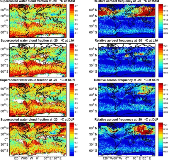
Figure 2.The global and seasonal variations of supercooled water cloud fractions (SCFs) and relative aerosol frequencies (RAFs) during nighttime at−20◦C isotherm over 2◦×2◦grid boxes.
in aerosol product) are removed from the dataset (approxi-mately 6 % of all aerosol layers). Meanwhile, GMAO tem-perature of aerosol layer top is also used here to select con-sistent temperature bins with the CALIPSO-GOCCP cloud product. For every IN aerosol sample, we arrange a tempera-ture bin based on its layer-top temperatempera-ture. Then, we define the frequency of IN aerosols at a given temperature bin as the ratio of the number of IN aerosol samples to the total num-ber of observation profiles for the same temperature bin and grid (Choi et al., 2010). Finally, the relative occurrence fre-quencies of IN aerosols are calculated by normalizing aerosol frequencies. That is, aerosol frequencies are divided by the highest aerosol frequency at a given isotherm (that is, tem-perature bin). The RAF is thus indicative of the temporal and spatial variability of IN aerosols compared to the maximum occurrence frequency (Choi et al., 2010).
Furthermore, considering the sparse sample data for the narrow CALIOP orbit, we reduce the horizontal resolution from 2 to 6◦ for ensuring enough samples in each grid
box when analyzing the relationship between SCFs and meteorological parameters under different aerosol loadings
(Sect. 3.2). To avoid artifacts due to noise from scattering of sunlight, only the nighttime datasets of cloud phase, meteoro-logical parameters and aerosol are used to perform following analysis.
3 Results
3.1 Global and seasonal distributions of 8-year average SCFs and RAFs
1852 J. Li et al.: Effects of dynamics and aerosols on the cold cloud phase
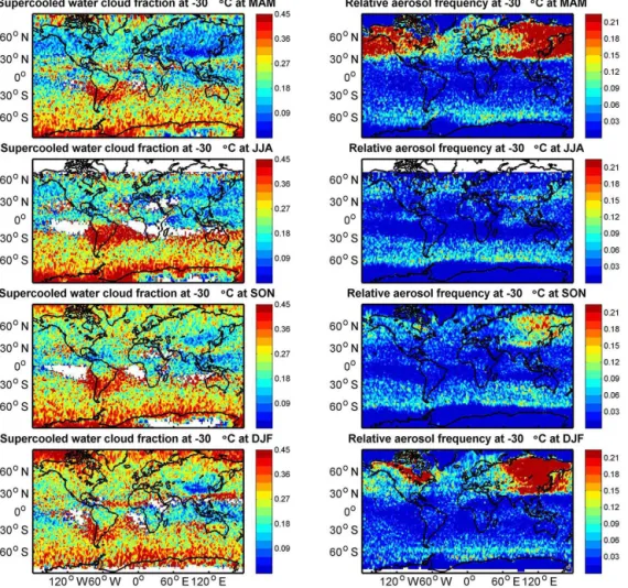
Figure 3.The global and seasonal variations of supercooled water cloud fractions (SCFs) and relative aerosol frequencies (RAFs) during nighttime at−30◦C isotherm over 2◦×2◦grid boxes.
Greenland. The SCFs between 30◦N and 30◦S range from approximately 55 to 75 %; the lowest SCFs (< 40 %) are pre-dominantly located in mainland China during boreal win-ter season, mostly in northweswin-tern and northeaswin-tern parts of China. For relative aerosol frequency at the−10◦C isotherm, its global distributions are expected and large RAFs are pre-dominantly located in the dust source regions, i.e., Saharan and Taklamakan deserts, where dust relative frequencies are greater than 20 % during boreal summer and spring, respec-tively. The “aerosol belt” near the US (between 30 and 60◦N)
during boreal spring is mostly from the long-range transport of dust from the Taklamakan Desert, which travels across the Pacific Ocean to the US via westerlies (Huang et al., 2008). In addition, Saharan dust can also be transported by trade winds across the Atlantic to the US and the Caribbean. At the −20 and−30◦C isotherms, the spatial patterns of SCFs are similar to those results at−10◦C and SCFs are lower at−20 and−30◦C than at−10◦C. However, the seasonal variation of SCFs at−20 and−30◦C is more obvious compared with those results at −10◦C, especially at high latitudes of the Northern Hemisphere. For RAFs, however, the comparison
between different isotherms is not meaningful because the RAFs are normalized relative to each fixed isotherm. Thus, larger RAF at−20 or−30◦C than at−10◦C does not mean that the true aerosol frequency at−20 or −30◦C is really higher than values at−10◦C. Compared with the RAFs at the−10◦C isotherms, the “aerosol belt” between 30 and 60◦ for two hemispheres at the−20 or−30◦C isotherms is more
apparent. Previous studies have verified that the regional dif-ferences in the SCFs at−20◦C or other isotherms are highly
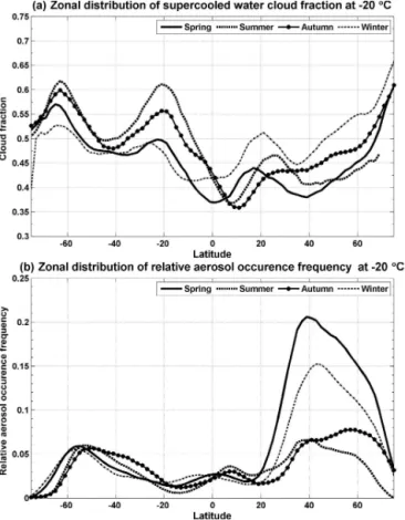
ex-Figure 4.The zonal and seasonal variations of SCFs and RAFs dur-ing nighttime at−20◦C isotherm.
plain all changes of the supercooled liquid cloud fraction in our study, especially its regional and seasonal variations. In other words, there is no evidence to suggest that the aerosol effect is always dominant at each isotherm or region. Then, can these variations of SCF attribute to the meteorological ef-fect? If yes, what is the role of meteorological parameters on the cloud phase change, especially at those regions in which the aerosol effect on nucleation is not first-order due to low IN aerosol frequency? In the following section, temporal and spatial correlation analysis between SCFs and meteorologi-cal parameters is conducted to help discuss these questions. 3.2 Temporal correlations between SCFs and
meteorological parameters
The synoptical-scale dynamics is the first-order variable driv-ing the formation of clouds and their properties (Noel et al., 2010). Aside from temperature, some past theoretical studies and observations already verified that the in-cloud updraft motions can supply a plentiful of water vapor for the persis-tence of cloud liquid, thus playing an important role in the cloud phase partitioning in mixed-phase clouds (Rauber and Tokay, 1991; Tremblay et al., 1996; Shupe at al., 2006). A sufficient updraft can be sourced by cloud top entrainment of dry air, radiative cooling, wing shear, larger-scale
insta-bilities and surface turbulent heat fluxes (Pinto, 1998; Mo-eng, 2000). In addition, Naud et al. (2006) also indicated that glaciation of supercooled water drops may be a func-tion of the large-scale vertical mofunc-tions, precipitafunc-tion, devel-opment stage of cloud and concentration of IN. In this sec-tion, we investigate the potential correlations between large-scale meteorological parameters and SCFs over the 8-year period (96 months). Although these statistical correlations do not imply complete causation, we expect that these results may provide a unique point of view on the phase change of mixed-phase cloud.
In view of the issue of a sparse dataset caused by the nar-row orbit of CALIOP, we perform the correlation analysis at 6◦latitude by 6◦longitude grid boxes. Firstly, we calcu-late the monthly averages of SCF, meteorological parameters and RAFs at different isotherms (or pressure levels) in each 6◦latitude by 6◦longitude grid box by using the following
equation:
M=
9 X i=1
wi ×Mi
! , 9
X i=1
wi,
whereMi is the averaged SCF or meteorological parameter of theith 2◦×2◦grid box in this 6◦×6◦geographic region, andwi=cos(θi×π/180.0); hereθi is the mean latitude of the ith 2◦×2◦ grid. Then, temporal correlations between monthly averaged SCFs and meteorological parameters are performed in each 6◦ latitude by 6◦ longitude grid box. It is worth noting that only those grid boxes whose temporal correlations are at the 90 % confidence level are displayed in the following global maps and are used further to discuss the spatial correlation in Sect. 3.3.
1854 J. Li et al.: Effects of dynamics and aerosols on the cold cloud phase
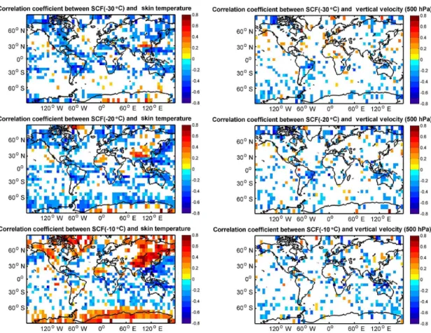
Figure 5.Temporal correlations (at the 90 % confidence level) between SCFs at three isotherms and skin temperature (left panel) and vertical velocity at 500 hPa (right panel). The correlations are based on 96 months’ monthly SCFs and meteorological parameters. Grid size is 6◦ latitude by 6◦longitude.
warm sea surface temperature and large-scale ascent (right panel of Fig. 5) are in favor of the ice formation. This re-sult is consistent with the study from Cesana et al. (2015), which found updrafts correspond to slightly warmer cloud phase transition than those downdrafts, and this relationship also can be found at different latitudes. Indeed, it is clear that the negative temporal correlations between SCFs and the vertical velocity at 500 hPa exist at almost all latitudes al-though grid boxes are considerably scattered. This might be because large-scale ascent in this study smooths many cloud-scale vertical motions. At middle latitudes, we also find a negative correlation between SCF and surface temperature except for mainland China. By analyzing the frontal clouds over the midlatitudes of the Northern Hemisphere, Naud et al. (2006) pointed out that the changes in glaciation temper-ature of supercooled liquid cloud appear to be related to the sea surface temperature (SST) pattern, storm vertical veloc-ity and strength. Glaciation of supercooled liquid cloud is likely to occur preferentially in the storm region where the warmer SST occurs. In these warm regions (e.g., tropics), strong precipitation rates may exhaust the supercooled liq-uid drops. Their finding possible partially explains the neg-ative correlations between SCF and skin temperature at the
Figure 6.Similar to Fig. 5 but for relative humidity (left panel) and LTSS (right panel).
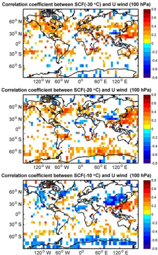
Similar to Fig. 5, Fig. 6 shows the temporal correlations between SCFs at three isotherms and LTSS, relative humid-ity at three pressure levels (400, 500 and 600 hPa). It is clear that SCFs at different regions and isotherms apparently neg-atively correlate with humidity. By analyzing the time series of perturbation for SCF and humidity (figure not shown), we find that their correlation is still obvious. It means that SCFs decrease as the relative humidity increases without regard to their region. This result also is consistent with study form Ce-sana et al. (2015). Besides the humidity, there is also obvious correlation between SCFs and LTSS (right panel of Fig. 6). We can see that the negative correlations between SCFs and LTSS mainly locate at the ocean region. It means that SCF is low in a stable low level atmosphere. For the horizontal wind speed at 100 hPa, Noel et al. (2010) found that the fre-quency of oriented crystal drops severely in areas dominated by stronger horizontal wind speed at 100 hPa. This effect is especially noticeable at latitudes below 40◦. However, they have not explained why the correlation between horizontal wind speed and horizontally oriented ice particle is negative. We speculate that strong horizontal wind possibly results in strong vertical wind shear, thus causing shear-gravitational wave motions to induce local updraft circulations (Rauber and Tokay, 1991). As a result, updraft possibly perturbs the orientation of ice crystal. In addition, Westbrook et al. (2010)
pointed out that supercooled liquid water layers is very im-portant in the formation of planar ice particles, which are sus-ceptible to orientation at midlatitudes. Based on these stud-ies, we assume that the temporal correlation between SCF and zonal wind speed also exists. Indeed, stronger winds are correlated with an increase in SCFs at different isotherms for ocean region of middle latitudes, whereas negative correla-tions also exist in central Africa, the Tibetan Plateau or pole-ward regions of 60◦S (see Fig. 7). All this being said, this section presents specifically the relationship between SCF and different meteorological parameters on a global scale rel-ative to some previous studies (e.g., Naud et al., 2006) which mainly focused on special regions, although we have not es-tablished a certain causal relationship in the present study. Noticeably, our statistical results demonstrate that the SCF variation is closely related to the meteorological parameters but their relationship is not stable and varies with the differ-ent regions, seasons and isotherm levels and thus should be treated carefully in the prediction of future climate change.
1856 J. Li et al.: Effects of dynamics and aerosols on the cold cloud phase
Figure 7.Similar to Fig. 5 but forUwind at 100 hPa.
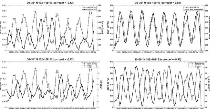
temporal correlation coefficients in the subplots of Figs. 8– 10 are calculated based on the original series, which has a greater than 90 % confidence level. We also provide the con-fidence value (i.e., p value) when the confidence level of the temporal correlation between variables is less than 90 %. Figure 8 shows the time series of various variables at the −30◦C isotherm over the central China (102–108◦E, 30– 36◦N), which is near to the Taklamakan Desert. High fre-quencies of dust and polluted dust in this region peak dur-ing the months when SCFs are at minimum with the cor-relation coefficient of−0.42. Negative correlations also ex-ist between SCF and LTSS (or horizontal wind at 100 hPa); their values are−0.17 and−0.53, respectively. In addition, the skin temperature over this region also display a coher-ent seasonal variation with the SCFs (corrcoef=0.58). At the−10◦C isotherm over a region near the Antarctic (174– 180◦E, 66–72◦S), the RAFs of aerosol are persistently low (< 0.02) for 96 months (see Fig. 9). The correlation coeffi-cient between SCF and RAF is only −0.09, and its confi-dence level is very low (P =0.39). The seasonal variations of SCF over this region are consistent with the meteorolog-ical parameters. For example, their correlation coefficients
are 0.22,−0.18 and−0.18 for skin temperature, LTSS and U wind, respectively. The third region is located over the Southern Ocean (116–122◦E, 18–24◦N), where the
maxi-mum RAF of aerosol at the−20◦C isotherm can reach 0.05 (see Fig. 10). Skin temperature and LTSS have negative cor-relations with SCF (−0.59 and 0.51, respectively), whereas a positive temporal correlation exists between SCF and U wind (approximately 0.45). These statistical results further indicate that the same meteorological parameter has a dis-tinct correlation with SCFs in different regions.
3.3 Spatial correlations between SCFs and meteorological parameters
In this section, we further investigate the spatial correlations of SCF and different meteorological parameters under dif-ferent aerosol loadings. As the correlations between SCFs and aerosol frequencies are less likely to be statistically sig-nificant in the Southern Hemisphere and tropics due to far fewer aerosols compared to the Northern Hemisphere, we only provide the global results. Here, each meteorological factor of grids is grouped into six bins based on its values within a specified aerosol loading level. In the present study, the aerosol loadings are divided into three levels based on rel-ative aerosol frequencies. The three aerosol levels are high level (RAF > 0.05), middle level (0 < RAF < 0.05) and low level (RAF=0). Such grouping ensures a sufficient number of samples available in each bin (at least several hundreds of samples in each bin) to satisfy statistical significance. More-over, note that only regions with temporal correlations of SCFs and meteorological parameters greater than the 90 % confidence level are used to calculate the spatial correlations between SCFs and meteorological parameters.
Figure 8.Time series plots of SCFs, meteorological parameters and RAFs of IN aerosol at−30◦C isotherm over the central China (102– 108◦E, 30–36◦N). Each line in every subplot corresponds to a time series of different variables after 5 months of smoothing. The coefficients (at the 90 % confidence level) in subplots represent the temporal correlation between the original SCFs series and meteorological parameters (or RAFs). The confidence values (i.e.,pvalue) are provided only when the confidence level of the temporal correlation between variables is less than 90 %.
1858 J. Li et al.: Effects of dynamics and aerosols on the cold cloud phase
Figure 10.Similar to Fig. 8 but for−20◦C isotherm over the subtropics of the Northern Hemisphere (116–122◦E, 18–24◦N).
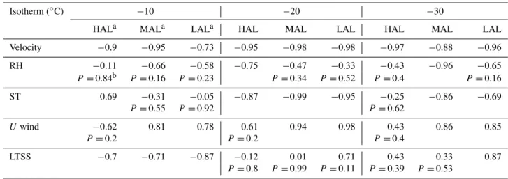
Table 1.The summary of spatial correlation coefficients between SCFs and meteorological parameters at three isotherms under different aerosol loading conditions. Only regions with temporal correlations between SCFs and meteorological parameters at the 90 % confidence level are used to calculate the spatial correlations between SCFs and meteorological parameters.
Isotherm (◦C) −10 −20 −30
HALa MALa LALa HAL MAL LAL HAL MAL LAL
Velocity −0.9 −0.95 −0.73 −0.95 −0.98 −0.98 −0.97 −0.88 −0.96
RH −0.11 −0.66 −0.58 −0.75 −0.47 −0.33 −0.43 −0.96 −0.65
P =0.84b P=0.16 P =0.23 P =0.34 P =0.52 P =0.4 P=0.16
ST 0.69 −0.31 −0.05 −0.87 −0.99 −0.95 −0.25 −0.86 −0.69
P=0.55 P =0.92 P =0.62
Uwind −0.62 0.81 0.78 0.61 0.94 0.98 0.43 0.86 0.85
P=0.2 P=0.2 P =0.4
LTSS −0.7 −0.71 −0.87 −0.12 0.01 0.71 0.43 0.33 0.87 P=0.8 P =0.99 P =0.11 P =0.39 P =0.53
aHAL, MAL and LAL are represent the high, middle and low aerosol loading levels;bWe also provide the confidence value (i.e.,pvalue) when the confidence level of
the spatial correlation between variables is less than 90 %.
firstly with increasing of humidity, then increase gradually, especially under the low aerosol loading condition. Similar to relative humidity, the SCF also decreases firstly with increas-ing of LTSS, then increases gradually. However, based on the Table 1, it is clear that the spatial correlation coefficients at a global scale between SCFs and relative humidity (or LTSS) are weak and the confidence level is not significant. It further indicates that the same meteorological parameter has a dis-tinct correlation with SCFs in different regions. Obvious spa-tial correlations also exist between SCFs and zonal wind at 100 hPa (Fig. 11e), especially under low and middle aerosol loading conditions. For example, the spatial correlations be-tween SCFs at−10◦C and zonal wind are−0.62, 0.81 and 0.78 for high, middle and low aerosol loadings, respectively. In summary, strong horizontal wind and low skin tempera-ture (or vertical velocity) correspond to high SCF. In Figs. 2 and 3, we find that the highest SCF does not mean the low-est aerosol frequency over this region (e.g., Southern Ocean). This further indicates that aerosol is not the unique factor to affect the seasonal cycles of SCF. Here, we emphasize that the statistical relationships between SCFs and meteoro-logical parameters are based on the long-term (96 months) datasets to ensure the correlations at the 90 % confidence are robust. From the above analysis and discussion, we are cer-tain that, at least, the variations of SCFs at a given isotherm are obviously correlated with the meteorological parameters, and their correlations depend on regions.
4 Conclusions and discussion
Changes in-cloud phase can significantly affect the Earth’s radiation budget and global hydrological cycle. Based on the 8 years (2007–2015) of cloud phase information dataset
from CALIPSO-GOCCP, aerosol products from CALIPSO and meteorological parameters from the ERA-Interim, this study investigates the effects of atmospheric dynamics on the supercooled liquid cloud fraction during nighttime under dif-ferent aerosol loadings at a global scale and achieve some new insights in this paper.
Previous studies mainly focused on warm water cloud sys-tems (Li et al., 2011, 2013; Kawamoto and Suzuki, 2012, 2013) or dust properties retrieval and simulations (Huang et al., 2010; Bi et al., 2011; Liu et al., 2011) or have demon-strated the importance of dust with respect to cloud proper-ties (Huang et al., 2006b, c, 2014; Su et al., 2008; Wang et al., 2010, 2015, 2016). Some studies have investigated the impact of different aerosol types on cold phase clouds over East Asia (Zhang et al., 2015) or at a global scale (Choi et al., 2010; Tan et al., 2014). However, studies of the statistical relationship between cloud phase changes and meteorologi-cal parameters have received far less attention, especially at a global scale. To clarify the roles of different meteorological factors in determining cloud phase changes and further pro-vide observational epro-vidence for the design and evaluation of a more physically based cloud phase partitioning scheme, we perform specially temporal and spatial correlations between SCFs and different meteorological factors on a global scale in this work.
tempo-1860 J. Li et al.: Effects of dynamics and aerosols on the cold cloud phase
ral correlations between SCFs versus vertical velocity and relative humidity indicate that the higher vertical velocity and relative humidity the smaller SCFs. The smaller SCFs are possibly due to strong precipitation exhausting the large supercooled liquid droplets. However, the impacts of LTSS, skin temperature and horizontal wind on SCFs are relatively complex than those of vertical velocity and humidity. Their temporal correlations with SCFs depend on latitude or sur-face type. For example, at the −10◦C isotherm, negative temporal correlations for skin temperature are mainly located in ocean regions between 30 and 60◦ for two hemispheres, whereas positive correlations can be found in the land region of high latitudes. With decreasing temperature (e.g., at the −20◦C isotherm), temporal correlation coefficients between SCFs and skin temperature are almost negative in middle and high latitudes. However, it is clear that their temporal correla-tions vary from positive to negative with decreasing temper-ature at some special regions (e.g., mainland China). By an-alyzing the spatial correlations under different aerosol load-ings, we find that negative correlations also exist between SCF and the vertical velocity (or surface skin temperature), whereas positive spatial correlations can be found between SCF and the U wind. Recently, evidence has shown that a cloud phase feedback occurs, causing more shortwave to be reflected back out to space relative to the state prior to global warming (McCoy et al., 2014, 2015). Our results, which are based on long-term (96 months) global observations, verify the effects of dynamic factors on cloud phase changes and illustrate that these effects are regional, thus having potential implications for further reducing the biases of climate feed-backs and climate sensitivity among climate models.
5 Data availability
The cloud phase product (CALIPSO-GOCCP) is available from the CFMIP-OBS website: ftp: //ftp.climserv.ipsl.polytechnique.fr/cfmip/GOCCP/3D_ CloudFraction/grid_2x2xL40/ (CALIPSO-GOCCP, 2016). The ERA-Interim reanalysis daily 6 h products are downloaded from the ERA-Interim website: http: //www.ecmwf.int/en/research/climate-reanalysis/era-interim (ERA-Interim, 2016). Aerosol data are obtained from the Atmospheric Science Data Center after registration at https: //eosweb.larc.nasa.gov/project/calipso/aerosol_layer_table, (CALIPSO-Aerosol, 2016).
Competing interests. The authors declare that they have no conflict of interest.
Acknowledgements. This research was jointly supported by the key Program of the National Natural Science Foundation of China (41430425), Foundation for Innovative Research Groups of the Na-tional Science Foundation of China (grant no. 41521004), NaNa-tional
Science Foundation of China (grant nos. 41575015, 41305027 and 41375031) and the China 111 project (grant no. B13045). We would like to thank the CALIPSO-GOCCP, CALIPSO and ERA-Interim science teams for providing excellent and accessible data products that made this study possible.
Edited by: J. Quaas
Reviewed by: two anonymous referees
References
Boucher, O., Randall, D., Artaxo, P., Bretherton,C., Feingold, G., Forster, P., Kerminen, V., Kondo, Y., Liao, H., Lohmann, U., Rasch, P., Satheesh, S. K., Sherwood, S., Stevens, B., and Zhang, X. Y.: Clouds and aerosols, in: Climate Change 2013: The Phys-ical Science Basis. Contribution of Working Group I to the Fifth Assessment Report of the Intergovernmental Panel on Climate Change, edited by: Stocker, T. F., Qin, D., Plattner, G.-K., Tig-nor, M., Allen, S. K., Boschung, J., Nauels, A., Xia, Y., Bex, V., and Midgley, P. M., 571–657, Cambridge Univ. Press, Cam-bridge, UK, New York, doi:10.1017/CBO9781107415324, 2013. Bey, I., Jacob, D. J., Yantosca, R. M., Logan, J. A., Field, B. D., Fiore, A. M., Li, Q., Liu, H. Y., Mickley, L. J., and Schultz, M. G.: Global modeling of tropospheric chemistry with assimilated meteorology: Model description and evaluation, J. Geophys. Res., 106, 23073–23095, doi:10.1029/2001JD000807, 2001. Bi, J., Huang, J., Fu, Q., Wang, X., Shi, J., Zhang, W., Huang, Z.,
and Zhang, B.: Toward characterization of the aerosol optical properties over Loess Plateau of Northwestern China, J. Quant. Spectrosc. Ra., 112, D00K17, doi:10.1029/2009JD013372, 2011.
Bodas-Salcedo, A., Webb, M. J., Bony, S., Chepfer, H., Dufresne, J.-L., Klein, S. A., Zhang, Y., Marchand, R., Haynes, J. M., Pin-cus, R., and John, V. O.: COSP: Satellite simulation software for model assessment, B. Am. Meteorol. Soc., 92, 1023–1043, doi:10.1175/2011BAMS2856.1, 2011.
Bower, K. N., Moss, S. J., Johnson, D. W., Choularton, T. W., Latham, J., Brown, P. R. A., Blyth, A. M., and Cardwell, J.: A parameterization of the ice water content observed in frontal and convective clouds, Q. J. Roy. Meteor. Soc., 122, 1815–1844, 1996.
CALIPSO-Aerosol: CALIPSO level 2, 5 km aerosol layer prod-uct, available at: https://eosweb.larc.nasa.gov/project/calipso/ aerosol_layer_table, last access: 20 December 2016.
CALIPSO-GOCCP: cloud phase product, available at: ftp://ftp.climserv.ipsl.polytechnique.fr/cfmip/GOCCP/3D_ CloudFraction/grid_2x2xL40/, last access: 20 December 2016. Cesana, G. and Chepfer, H.: How well do climate models simulate
cloud vertical structure? – A comparison between CALIPSO-GOCCP satellite observations and CMIP5 models, Geophys. Res. Lett., 39, L20803, doi:10.1029/2012GL053153, 2012. Cesana, G. and Chepfer, H.: Evaluation of the cloud water phase
in a climate model using CALIPSO-GOCCP, J. Geophys. Res.-Atmos., 118, 7922–7937, doi:10.1002/jgrd.50376, 2013. Cesana, G., Kay, J. E., Chepfer, H., English, J. M., and
from CALIPSO-GOCCP, Geophys. Res. Lett., 39, L20804, doi:10.1029/2012GL053385, 2012.
Cesana, G., Waliser, D. E., Jiang, X., and Li, J.-L. F.: Multi-model evaluation of cloud phase transition using satellite and reanalysis data, J. Geophys. Res.-Atmos., 120, 7871–7892, doi:10.1002/2014JD022932, 2015.
Cesana, G., Chepfer, H., Winker, D., Cai, X., Getzewich, B., Okamoto, H., Hagihara, Y., Jourdan, O., Mioche, G., Noel, V., and Reverdy, M.: Using in-situ airborne mea-surements to evaluate three cloud phase products derived from CALIPSO, J. Geophys. Res.-Atmos., 121, 5788–5808, doi:10.1002/2015JD024334, 2016.
Chepfer, H., Bony, S., Winker, D. M., Chiriaco, M., Dufresne, J.-L., and Seze, G.: Use of CALIPSO lidar observations to evaluate the cloudiness simulated by a climate model, Geophys. Res. Lett., 35, L15704, doi:10.1029/2008GL034207, 2008.
Chepfer, H., Bony, S., Winker, D., Cesana, G., Dufresne, J. L., Min-nis, P., Stubenrauch, C. J., and Zeng, S.: The GCM Oriented Calipso Cloud Product (CALIPSO-GOCCP), J. Geophys. Res., 115, D00H16, doi:10.1029/2009JD012251, 2010.
Chepfer, H., Cesana, G., Winker, D., Getzewich, B., Vaughan, M., and Liu, Z.: Comparison of two different cloud climatologies de-rived from CALIOP Level 1 observations: The CALIPSO-ST and the CALIPSO-GOCCP, J. Atmos. Ocean. Tech., 30, 725– 744, doi:10.1175/JTECH-D-12-00057.1, 2013.
Choi, Y. S., Lindzen, R. S., Ho, C. H., and Kim, J.: Space observa-tions of cold-cloud phase change, P. Natl. Acad. Sci. USA, 107, 11211–11216, 2010.
Choi, Y.-S., Ho, C.-H., Park, C.-E., Storelvmo, T., and Tan I.: Influence of cloud phase composition on cli-mate feedbacks, J. Geophys. Res.-Atmos., 119, 3687–3700, doi:10.1002/2013JD020582, 2014.
Cziczo, D. J., Froyd, K. D., Hoose, C., Jensen, E. J., Diao, M., Zondlo, M. A., Smith, J. B., Twohy, C. H., and Mur-phy, D. M.: Clarifying the dominant sources and mecha-nisms of cirrus cloud formation, Science, 340, 1320–1324, doi:10.1126/science.1234145, 2013.
Dee, D. P., Uppala, S. M., Simmons, A. J., Berrisford, P., Poli, P., Kobayashi, S., Andrae, U., Balmaseda, M. A., Balsamo, G., Bauer, P., Bechtold, P., and Beljaars, A. C. M.: The ERA-Interim reanalysis: Configuration and performance of the data assimila-tion system, Q. J. Roy. Meteor. Soc., 137, 553–597, 2011. Delanoe, J. and Hogan, R. J.: Combined CloudSat–CALIPSO–
MODIS retrievals of the properties of ice clouds, J. Geophys. Res.-Atmos., 115, D00H29, doi:10.1029/2009JD012346, 2010. ERA-Interim: ERA-Interim reanalysis daily 6 h products,
avail-able at: http://www.ecmwf.int/en/research/climate-reanalysis/ era-interim, last access: 20 December 2016.
Hu, Y., Vaughan, M., Liu, Z., Lin, B., Yang, P., Flittner, D., Hunt, W., Kuehn, R., Huang, J., Wu, D., Rodier, S., Powell, K., Trepte, C., and Winker, D.: The depolarization-attenuated backscatter re-lation: CALIPSO lidar measurements vs. theory, Opt. Exp., 15, 5327–5332, 2007.
Hu, Y., Winker, D., Vaughan, M., Lin, B., Omar, A., Trepte, C., Flittner, D., Yang, P., Nasiri, S., Baum, B. A., Sun, W., Liu, Z., Wang, Z., Young, S., Stamnes, K., Huang, J., Kuehn, R., and Holz, R. E.: CALIPSO/CALIOP cloud phase discrim-ination algorithm, J. Atmos. Ocean. Tech., 26, 2206–2309, doi:10.1175/2009JTECHA1280.1, 2009.
Hu, Y., Rodier, S., Xu, K. M., Sun, W., Huang, J., Lin, B., Zhai, P., and Josset, D.: Occurrence, liquid water content, and fraction of supercooled water clouds from combined CALIOP/IIR/MODIS measurements, J. Geophys. Res., 115, D00H34, doi:10.1029/2009JD012384, 2010.
Huang, J. P., Minnis, P., and Lin, B.: Advanced retrievals of mul-tilayered cloud properties using multispectral measurements, J. Geophys. Res., 110, D15S18, doi:10.1029/2004JD005101, 2005. Huang, J. P., Minnis, P., and Lin, B.: Determination of ice water path in ice-over-water cloud systems using combined MODIS and AMSR-E measurements, Geophys. Res. Lett., 33, L21801, doi:10.1029/2006GL027038, 2006a.
Huang, J. P., Lin, B., Minnis, P., Wang, T., Wang, X., Hu, Y., Yi, Y., and Ayers, J. R.: Satellite-based assessment of possible dust aerosols semi-direct effect on cloud water path over East Asia, Geophys. Res. Lett., 33, L19802, doi:10.1029/2006GL026561, 2006b.
Huang, J. P., Minnis, P., Lin, B., Wang, T., Yi, Y., Hu, Y., Sun-Mack, S., and Ayers, K.: Possible influences of Asian dust aerosols on cloud properties and radiative forcing observed from MODIS and CERES, Geophys. Res. Lett., 33, L06824, doi:10.1029/2005GL024724, 2006c.
Huang, J. P., Minnis, P., Chen, B., Huang, Z., Liu, Z., Zhao, Q., Yi, Y., and Ayers, J. K.: Long-range transport and verti-cal structure of Asian dust from CALIPSO and surface mea-surements during PACDEX, J. Geophys. Res., 113, D23212, doi:10.1029/2008JD010620, 2008.
Huang, J. P., Wang, T., Wang, W., Li, Z., and Yan, H.: Climate effects of dust aerosols over East Asian arid and semiarid regions, J. Geophys. Res., 119, 11398–11416, doi:10.1002/2014JD021796, 2014.
Huang, Z., Huang, J., Bi, J., Wang, G., Wang, W., Fu, Q., Li, Z., Tsay, S.-C., and Shi, J.: Dust aerosol vertical structure measurements using three MPL lidars during 2008 China-U.S. joint dust field experiment, J. Geophys. Res., 115, D00K15, doi:10.1029/2009JD013273, 2010.
Jiang, H., Cotton, W. R., Pinto, J. O., Curry, J. A., and Weissbluth, M. J.: Cloud resolving simulations of mixed-phase Arctic stratus observed during BASE: Sensitivity to concentration of ice crys-tals and large-scale heat and moisture advection, J. Atmos. Sci., 57, 2105–2117, 2000.
Kawamoto, K. and Suzuki, K.: Microphysical transition in wa-ter clouds Over the Amazon and China derived from space-borne radar and Radiometer data, J. Geophys. Res., 117, D05212, doi:10.1029/2011JD016412, 2012.
Kawamoto, K. and Suzuki, K.: Comparison of water cloud mi-crophysics over mid-latitude land and ocean using CloudSat and MODIS observations, J. Quant. Spectrosc. Ra., 122, 13–24, 2013.
Klein, S. A. and Hartmann, D. L.: The seasonal cycle of low strati-form clouds, J. Climate, 6, 1588–1606, 1993.
Li, J., Yi, Y., Minnis, P., Huang, J., Yan, H., Ma, Y., Wang, W., and Ayers, J. K.: Radiative effect differences between multi-layered and single-layer clouds derived from CERES, CALIPSO, and CloudSat data, J. Quant. Spectrosc. Ra., 112, 361–375, doi:10.1016/j.jqsrt.2010.10.006, 2010.
1862 J. Li et al.: Effects of dynamics and aerosols on the cold cloud phase
by using the tail of the CALIOP signal, Atmos. Chem. Phys., 11, 2903–2916, doi:10.5194/acp-11-2903-2011, 2011.
Li, J., Yi, Y. H., Stamnes, K., Ding, X. D., Wang, T. H., Jin, H. C., and Wang, S. S.: A new approach to retrieve cloud base height of marine boundary layer clouds, Geophys. Res. Lett., 40, 4448– 4453, doi:10.1002/grl.50836, 2013.
Li, J., Huang, J., Stamnes, K., Wang, T., Lv, Q., and Jin, H.: A global survey of cloud overlap based on CALIPSO and CloudSat mea-surements, Atmos. Chem. Phys., 15, 519–536, doi:10.5194/acp-15-519-2015, 2015.
Liu, Y., Huang, J., Shi, G., Takamura, T., Khatri, P., Bi, J., Shi, J., Wang, T., Wang, X., and Zhang, B.: Aerosol optical properties and radiative effect determined from sky-radiometer over Loess Plateau of Northwest China, Atmos. Chem. Phys., 11, 11455– 11463, doi:10.5194/acp-11-11455-2011, 2011.
Liu, Z., Vaughan, M., Winker, D., Kittaka, C., Getzewich, B., Kuehn, R., Omar, A., Powell, K., Trepte, C., and Hostetler, C.: The CALIPSO lidar cloud and aerosol dis-crimination: Version 2 algorithm and initial assessment of performance, J. Atmos. Ocean. Tech., 26, 1198–1213, doi:10.1175/2009JTECHA1229.1, 2009.
Lv, Q., Li, J., Wang, T., and Huang, J.: Cloud radiative forc-ing induced by layered clouds and associated impact on the atmospheric heating rate, J. Meteor. Res., 29, 779–792, doi:10.1007/s13351-015-5078-7, 2015.
Lohmann, U. and Feichter, J.: Global indirect aerosol effects: a re-view, Atmos. Chem. Phys., 5, 715–737, doi:10.5194/acp-5-715-2005, 2005.
McCoy, D. T., Hartmann, D. L., and Grosvenor, D. P.: Observed Southern Ocean Cloud Properties and Shortwave Reflection Part 2: Phase changes and low cloud feedback, J. Climate, 27, 8858– 8868, doi:10.1175/JCLI-D-14-00288.1, 2014.
McCoy, D. T., Hartmann, D. L., Zelinka, M. D., Ceppi, P., and Grosvenor, D. P.: Mixed-phase cloud physics and Southern Ocean cloud feedback in climate models, J. Geophys. Res.-Atmos., 120, doi:10.1002/2015JD023603, 9539–9554, 2015. Mielonen, T., Arola, A., Komppula, M., Kukkonen, J.,
Koski-nen, J., de Leeuw, G., and LehtiKoski-nen, K. E. J.: Comparison of CALIOP level 2 aerosol subtypes to aerosol types derived from AERONET inversion data, Geophys. Res. Lett., 36, L18804, doi:10.1029/2009GL039609, 2009.
Moeng, C.-H.: Entrainment rate, cloud fraction, and liquid water path of PBL stratocumulus cloud, J. Atmos. Sci., 57, 3627–3643, doi:10.1175/1520-0469(2000)057<3627:ERCFAL>2.0.CO;2, 2000.
Naud, C. M., Del Genio, A. D., and Bauer, M.: Observational con-straints on the cloud thermodynamic phase in midlatitude storms, J. Climate, 19, 5273–5288, 2006.
Niedermeier, D., Hartmann, S., Clauss, T., Wex, H., Kiselev, A., Sullivan, R. C., DeMott, P. J., Petters, M. D., Reitz, P., Schneider, J., Mikhailov, E., Sierau, B., Stetzer, O., Reimann, B., Bundke, U., Shaw, R. A., Buchholz, A., Mentel, T. F., and Stratmann, F.: Experimental study of the role of physicochemical surface pro-cessing on the IN ability of mineral dust particles, Atmos. Chem. Phys., 11, 11131–11144, doi:10.5194/acp-11-11131-2011, 2011. Noel, V. and Chepfer, H.: A global view of horizontally oriented crystals in ice clouds from Cloud-Aerosol Lidar and Infrared Pathfinder Satellite Observation (CALIPSO), J. Geophys. Res., 115, D00H23, doi:10.1029/2009JD012365, 2010.
Omar, A. H., Winker, D. M., Vaughan, M. A., Hu, Y., Trepte, C. R., Ferrare, R. A., Lee, K.-P., Hostetler, C. A., Kit-taka, C., Rogers, R. R., Kuehn, R. E., and Liu, Z.: The CALIPSO automated aerosol classification and lidar ratio se-lection algorithm, J. Atmos. Ocean. Tech., 26, 1994–2014, doi:10.1175/2009JTECHA1231.1, 2009.
Pinto, J. O.: Autumnal mixed-phase cloudy boundary layers in the Arctic, J. Atmos. Sci., 55, 2016–2038, 1998.
Pruppacher, H. R. and Klett, J. D.:Microphysics of Clouds and Pre-cipitation, 2nd ed., 954 pp., Kluwer Acad., Dordrecht, Nether-lands, 1997.
Rauber, R. M. and Tokay, A.: An explanation for the existence of supercooled water at the top of cold clouds, J. Atmos. Sci., 48, 1005–1023, 1991.
Sassen, K. and Khvorostyanov, V. I.: Microphysical and radiative properties of mixed phase altocumulus: a model evaluation of glaciation effects, Atmos. Res., 84, 390–398, 2007.
Shupe, M. D., Matrosov, S. Y., and Uttal, T.: Arctic mixed-phase cloud properties derived from surface-based sensors at SHEBA, J. Atmos. Sci., 63, 697–711, 2006.
Shupe, M. D., Kollias, P., Persson, P. O. G., and McFarquhar, G. M.: Vertical motions in arctic mixed phase stratus, J. Atmos. Sci., 65, 1304–1322, 2008.
Stephens, G. L., Vane, D. G., Boain, R. J., Mace, G. G., Sassen, K., Wang, Z., Illingworth, A. J., O’Connor, E. J., Rossow, W. B., Durden, S. L., Miller, S. D., Austin, R. T., Benedetti, A., Mitrescu, C., and CloudSat Science Team: The CloudSat mission and the A-Train, A new dimension of space-based observations of clouds and precipitation, B. Am. Meteorol. Soc., 83, 1771– 1790, 2002.
Su, J., Huang, J., Fu, Q., Minnis, P., Ge, J., and Bi, J.: Estimation of Asian dust aerosol effect on cloud radiation forcing using Fu-Liou radiative model and CERES measurements, Atmos. Chem. Phys., 8, 2763–2771, doi:10.5194/acp-8-2763-2008, 2008. Sun, Z. and Shine, K. P.: Studies of the radiative properties of ice
and mixed-phase clouds, Q. J. Roy. Meteor. Soc., 120, 111–137, 1994.
Tan, I., Storelvmo, T., and Choi, Y. S.: Spaceborne lidar observa-tions of the ice-nucleating potential of dust, polluted dust and smoke aerosols in mixed-phase clouds, J. Geophys. Res.-Atmos., 119, 6653–6665, doi:10.1002/2013JD021333, 2014.
Tan, I., Storelvmo, T., and Zelinka, M. D.: Observational constraints on mixed-phase clouds imply higher climate sensitivity, Science, 352, 224–227, 2016.
Tremblay, A., Glazer, A., Yu, W., and Benoit, R.: A mixed-phase cloud scheme based on a single prognostic equation, Tellus, 48A, 483–500, 1996.
Tsushima, Y., Emori, S., Ogura, T., Kimoto, M., Webb, M. J., Williams, K. D., Ringer, M. A., Soden, B. J., Li, B., and An-dronova, N.: Importance of the mixed phase cloud distribution in the control climate for assessing the response of clouds to carbon dioxide increase: a multi-model study, Clim. Dynam., 27, 113– 126, 2006.
Wang, W., Sheng, L., Jin, H., and Han, Y.: Dust Aerosol Effects on Cirrus and Altocumulus Clouds in Northwest China, J. Meteor. Res., 29, 793–805, 2015.
Wang, W., Sheng, L., Dong, X., Qu, W., Sun, J., Jin, H., and Logan, T.: Dust aerosol impact on the retrieval of cloud top height from satellite observations of CALIPSO, Cloud-Sat and MODIS, J. Quant. Spectrosc. Ra., 188, 132–141, doi:10.1016/j.jqsrt.2016.03.034, 2016.
West, R. E. L., Stier, P., Jones, A., Johnson, C. E., Mann, G. W., Bellouin, N., Partridge, D. G., and Kipling, Z.: The importance of vertical velocity variability for estimates of the indirect aerosol effects, Atmos. Chem. Phys., 14, 6369–6393, doi:10.5194/acp-14-6369-2014, 2014.
Westbrook, C. D., Illingworth, A. J., O’Connor, E. J., and Hogan, R. J.: Doppler lidar measurements of oriented planar ice crystals falling from supercooled and glaciated layer clouds, Q. J. Roy. Meteor. Soc., 136, 260–276, 2010.
Winker, D. M., Hunt, W. H., and Mcgill, M. J.: Initial perfor-mance assessment of CALIOP, Geophys. Res. Lett., 34, L19803, doi:10.1029/2007GL030135, 2007.
Zhang, D., Wang, Z., and Liu, D.: A global view of midlevel liquid-layer topped stratiform cloud distribution and phase partition from CALIPSO and CloudSat measurements, J. Geophys. Res., 115, D00H13, doi:10.1029/2009JD012143, 2010.