MASTER THESIS PRESENTED BY WILDER LEONARDO GAMBOA RUIZ
Angels Sahuquillo Estrugo, Professor in the Department of Analytical Chemistry at University of Barcelona,
ATTEST
That current work entitled
“Speciation of Mercury in Environmental Samples.”
Has been conducted by Wilder Leonardo Gamboa Ruiz in the Department of Analytical Chemistry at University of Barcelona under her supervision.
Acknowledgements
It is a pleasure to thank the many people involved in one or the other way in this work. I want to thank all of them, including those not mentioned here by name.
I would like to thank my supervisor, Dr. Angels Sahuquillo for her enthusiasm, inspiration, and great efforts to explain things clearly and simply. Throughout my thesis-writing period, she provided encouragement, advice, good teaching and lots of good ideas. I would have been lost without her. I wish to thank Dr. Fermín.López for his feedback during the development of this work
I am grateful to all the fellows of the Questram group for their company, support and all the good moments we share inside and outside of the lab. I wish to thank specially Carmen Ibañez; she has provided assistance in numerous ways, her dedication and boundless patience at every stage of the thesis process, allowed me to complete this project on schedule.
I wish to thank all the people involved in the Erasmus Mundus programme for giving me this opportunity; especially Dr. Isabel Cavaco for her guidance and concern during the entire master. I want to express my gratitude to all my EMQAL fellows. These individuals always helped me to keep my life in context. Graduate school isn't the most important thing in life, but good friends, good times and happiness are.
Lastly, and most importantly, I wish to thank my family for providing a loving environment. My parents: Flor and Victor and my dear brother Oswaldo. To them I dedicate this thesis and every little step in my life.
TABLE OF CONTENTS
1. INTRODUCTION
1.1 Mercury in the environment ... 12
1.2 Mercury Toxicity ... 13
1.3 Distribution of Mercury in the environment ... 14
1.4 Sample pretreatment for mercury speciation ... 16
1.5 Separation techniques for mercury speciation ... 17
2.1 Procedures ... 20
2.1.1 Sample description and sampling ... 20
2.1.2 Sample Pre-treatment ... 20
2.1.3 Moisture and Major Components ... 22
2.1.4 Aqua Regia Mercury Extraction (ISO 11466) ... 22
2.1.5 Microwave Mercury Extraction (EPA 3200) ... 23
2.1.6 Methyl, Ethyl and Inorganic Mercury Determination:... 24
2.1.7 Total Mercury Determination... 25
2.1.8 Labware cleaning ... 25
2. EXPERIMENTAL 2.2 Instruments ... 25
2.2.1 Description of the mercury analysis system ... 25
2.2.2 Equipments ... 28
2.2.3 Reagents and standards ... 29
2.2.3.1 Standards ... 29
2.2.3.2 Reagents ... 29
3. RESULTS AND DISCUSSION
3.1 Analytical Metodology for of Hg2+, MeHg+ and EtHg+ determination in waters. ... 32
3.1.1 Optimisation of the mobile phase composition ... 32
3.1.2 Establishment of the quality parameters ... 33
3.1.2.1 Calibration Curves ... 33
3.1.3 Detection and Quantification Limits ... 34
3.1.4 Recovery studies ... 35
3.1.5 Stability studies for EtHg+ ... 38
3.2 Analytical especiation of mercury in sediment: Effect of sample pre-treatment .... 40
3.2.1 Sample Characterization ... 40
3.2.2 Comparison of Different Sample Pre-treatment Procedures ... 42
3.2.3 Effect of sample pre-treatment on heavy metal determination. ... 47
CONCLUSIONS...49 REFERENCES...51
9
ABSTRACT
Mercury is one of the most toxic elements impacting on human and ecosystem health and therefore is one of the most studied environmental pollutants. All mercury species are toxic, with organic mercury compounds generally being more toxic than inorganic species. For this reason, the assessment of mercury distribution in environmental samples is a key task in analytical chemistry.
Reverse phase chromatography (RPC) coupled to a UV post-column oxidation system and vapor generation atomic fluorescence spectrometry was optimised for the speciation and determination of inorganic and organic mercury (methylmercury and ethylmercury) in the form of APDC complexes. The mercury-APDC complexes were separated on a reverse phase column and oxidized on-line with a UV source. Hg2+ was selectively detected by AFS after reduction with stannous chloride to Hg0. The mobile phase composition was modified to include the simultaneous detection of EtHg+ by optimising the MeOH – Water to a 75:25 ratio. Quality parameters for the analytical method were established and a short-term stability study for EtHg+ was undertaken.
Investigations are described to select the most suitable pre-treatment procedure for mercury speciation in polluted sediment samples. Five different pre-treatment procedures were evaluated: freezing at -80 and -20 °C, air drying, oven-drying at 40 °C, and lyophilization. Total mercury determination was performed with an aqua regia extraction, while for mercury speciation a method formerly optimized for the speciation of Hg2+ and MeHg+ was used in the analysis of sediments. The chromatogfraphic system consists on a reverse phase column (C18), with a mobile phase composed of
(80:20) MeOH – water containing APDC 0,0015M as complexing agent and HN4Ac
0,01M at pH 5,5. For total mercury measurement, best results were obtained when the sediments were dried (air dried, oven-dried or lyophilized) because frozen samples showed lower concentration of total mercury. In the case of speciation analysis, MeHg+ was not detected in the sediment samples. Significant differences were found in the Hg2+ concentration among the samples subjected to the studied pre-treatments, even if there is no evidence suggesting that one pre-treatment preserves better the original speciation information was found.
10
11
1 INTRODUCTION
12
1.1 Mercury in the environment
Nowadays, one of the most important issues linked with the assessment of the environmental pollution due to anthropogenic activities is the detection of heavy metals. Despite of the abundant evidence regarding the harmful effects which can be produced by the heavy metals in the health (1,2) and their strong environmental impact since they are cumulative and non-biodegradable, exposure to them continues due to the lack of both environmentally friendly practices and concrete prevention policies.
Within the group of heavy metals, Mercury (Hg) is one of the most dangerous environmental pollutants, which has been recognized as a potential environmental and public health problem for over 40 years. It is widely considered as one of the pollutants which generates more concern and receive a high global priority because is present in a diversity of chemical and physical forms with a wide variety of properties that determine its complex distribution, bioconcentration and toxicity.
Regardless of the recurrent problems related to the occupational exposure to inorganic mercury, during recent years, research of this pollutant has focused on identifying its potential impact on larger groups of the population due to the wide distribution of mercury in the environment.
Mercury exists in three oxidation states: Hg° (metallic), Hg+ (mercurous) and Hg2+ (mercuric) mercury. The latter forms a variety of inorganic as well as organometallic compounds. In the case of organometallic derivatives, the mercury atom is covalently bound to one or two carbon atoms. Mercury is emitted to the atmosphere by natural degassing of the earth’s surface and by reevaporation of mercury vapor previously deposited on the earth’s surface, in the form of elemental vapour (Hg°).
Anthropogenic sources of mercury are numerous and worldwide. Mercury is produced by the mining and smelting of cinnabar ore. It is used in chloralkali plants (producing chlorine and sodium hydroxide), in paints as preservatives or pigments, in electrical switching equipment and batteries, in measuring and control equipment (thermometers,
13
medical equipment), in mercury vacuum apparatus, as a catalyst in chemical processes, in mercury quartz and luminescent lamps, in the production and use of high explosives, in copper and silver amalgams in tooth-filling materials, and as fungicides in agriculture. (3)
Although all the species of mercury are toxic, the effects are closely related to its chemical form. The most environmentally interesting species are elemental mercury (Hg°), inorganic Hg (Hg2+), monomethylmercury (CH3Hg+, MeHg+),
monoethylmercury (CH3CH2Hg+, EtHg+) and dimethylmercury (CH3HgCH3, DMeHg).
In the biogeochemical cycle of Hg, these species may be transformed into each other and dynamically transported through the terrestrial, aquatic and atmospheric environmental compartments. The most relevant process suffered from mercury in the environment is the transformation of inorganic mercury into methylmercury (in this thesis, methylmercury refers to monomethyl mercury if not stated otherwise) by sulphate-reducting bacteria and the subsequent accumulation through the aquatic food chain attaining its highest concentrations in large predatory species at the top of the aquatic food-chain. By this way, it enters to the human diet. This situation leads to the mercury bioconcentration by hundred or thousand fold and cause a potential risk to humans (4).
1.2 Mercury Toxicity
Mercury has a unique volatility among the elements. This makes it quite mobile in the environment. This mobility is further enhanced because it can be methylated biologically (primarily by aquatic bacteria). Methylated Hg has special chemical characteristics (due to the methyl group) that make it prone to bioaccumulate in animals and plants; in contrast, inorganic Hg does not bioaccumulate. Methylmercury is considerably more toxic than elemental mercury and its inorganic salts, because it is efficiently adsorbed from the gastrointestinal tract due to its lyphophilicity, it is rapidly transported through biological membranes and accumulates on the surface of nerve cells causing neuronal damage (5).
14
The generally recognized adverse effects attributed to the Hg exposure, are stomatitis, erethism, and renal damage (for oral exposure). Toxic responses, such as axial malformations, stunting, neurological deficits, decreased of weight, altered enzyme levels, and renal failure, are examples of chemically induced effects of Hg exposure. Targets of inorganic mercury include proteins, which bind mercuric ions to sulfhydryl groups resulting in structural and catalytic protein alteration. Inorganic mercury is a central nervous system and renal toxicant. In contrast, methyl mercury is well-absorbed across membranes and is efficiently accumulated by biota. The primary target of methyl mercury toxicity is the central nervous system. Methyl mercury accumulates in muscle tissue where it binds to sulfhydryl groups of muscle proteins (6)
1.3 Distribution of Mercury in the environment
Mercury can cycle in the environment as a part of both natural and anthropogenic activities. As mercury cycles between the atmosphere, land and water, mercury undergoes a series of complex biological, chemical and physical transformations, and some of them are not completely understood. Humans, plants and animals are routinely exposed to mercury and accumulate it during this cycle, potentially resulting in a variety of ecological and human health impacts (7,8)
Recently, interest has grown about the biogeochemistry of mercury in the environment. In the atmosphere, where approximately 95% of total mercury is in the elemental state, it is slowly oxidized to the mercuric state. Hgo can circulate in the atmosphere for up to a year, and hence can be widely dispersed and transported thousands of miles from sources of emission. As a result, while the principal emissions of mercury are from punctual sources concentrated in industrial regions, mercury pollution is global. The return of mercury from the atmosphere to the Earth’s surface occurs mainly via wet precipitation of dissolved Hg2+ (see figure 1) (9).
Once oxidized, 60% of atmospheric mercury is deposited to land and 40% to water, even though land represents only 30% of the Earth’s surface (9). In oceanic waters, after it undergoes a complex set of chemical and biological transformations, most of the Hg2+
15
is reduced to Hg0 and returned to the atmosphere; only a small fraction is permanently exported to the sediments. Inorganic mercury can be methylated to mono- and dimethylmercury . Laboratory and field studies have shown the methylation of Hg2+ mainly by micro-organisms.
Figure 1. Global cycle of Mercury. The width of the arrows is proportional to the importance of the fluxes. (Adapted from reference 9)
In the waters the levels of methylmercury are usually much lower than those of inorganic mercury. This is due to the difficulty of methylation reactions in aqueous phases, from one side, and to the easy decomposition by solar UV light of organomercury compounds from the other. In sediments and biota the levels of methylmercury are higher than in waters because of accumulative phenomena.
Soils and sediments constitute concentrated reservoirs of trace metals in which the amounts are higher than those present in other environmental compartments, such as water. The concentrated pollutants can be potentially released due to changes in the physicochemical conditions. For this reason a key factor in the assessment of environmental risk is the evaluation of the total concentration of the metals and even
16
more important, their speciation and distribution among the different phases of these solid matrices. Taking into account the high affinity of the inorganic mercury for sulfides, it is logical to expect that this strong binding controls the chemistry of mercury in sediments and anoxic waters.
1.4 Sample pretreatment for mercury speciation
The procedure for sample preparation in speciation studies depends on the analytical technique to be used, on the sample type to be analyzed and on the analyte itself. The polarity or volatility of the analyte determines the technique to be chosen for the separation of the species prior to detection. The separation technique, on its turn, sets the requirements for the analyte solution resulting from the sample preparation procedure. Sample preparation practices generally include drying, filtration, grinding, solubilization, leaching, preconcentration, clean up and derivatization (10).
In the case of the speciation of mercury in soils and sediments, one of the key steps is the drying. Taking into account the volatility of some mercury species this step may give rise losses and change the original distribution of the mercury leading to erroneous results, even if the subsequent preparation steps are carried out effectively.
Different methods of preserving soils and sediments have been applied, i.e. wet at room temperature, wet at lowered temperature, frozen, freeze-dried, oven-dried, microwave oven-dried and air-dried at room temperature. The most convenient method should comply with certain requirements like the preservation of the original mercury speciation, allowing to obtain a homogeneous sample and minimized the storage problem.
There is still much debate on the effect of sample pretreatment on the MeHg+ and total mercury levels obtained. In some cases, no differences were found between fresh sediments and dried (lyophilized) sediments, whereas, in other cases, much higher results were found in dried sediments compared to wet sediments (11-13). Further investigation in this field is required.
17
1.5 Separation techniques for mercury speciation
After searching in the available literature, it is clear that one of the most applied techniques to perform mercury speciation studies in environmental samples is chromatography (both GC and LC) coupled to different detection systems. Several extraction methods have been proposed. These chromatographic techniques are used to measure the different organo-mercuric compounds.
In GC methods, the environmental sample must be extracted in order to obtain the organomercuric compounds. The most commonly used procedures for the extraction of organomercury species from environmental samples are acid extraction (mostly combined with solvent extraction), distillation and alkaline extractions. The extraction step is still one of the most critical steps and, for biota and sediments, almost certainly the most critical. The extraction involves several problems related with the extraction efficiency, conversion and destruction of the mercury species and moreover, the more common GC detectors may lack the required selectivity to be used for the speciation of Hg in environmental samples.
In order to overcome these problems, alternative methods have been developed involving precolumn derivatization of Hg species. The non-polar derivatives can then be separated on non-polar packed or capillary columns. Iodation with acetic acid, hydration with NaBH4, aqueous phase ethylation with NaBEt4, chlorination and derivatization
with a Grignard reagent, are the most commonly used methods (14,15).
In the case of LC methods, until recently, their main disadvantage was the poor sensitivity of the detectors. Development of more sensitive detectors, such as a reductive amperometric electrochemical, ultraviolet (UV), ICP-AES, ICP-MS, AFS and AAS, has resulted in wider applications in environmental studies. The main advantage of LC over a number of methods is the possibility of separating a great variety of organomercury compounds. Practically all HPLC methods for Hg speciation reported in the literature are based on reversed phase separations, involving the use of a silica-bonded phase column and a mobile phase containing an organic modifier, a chelating or ion-pair reagent and, in some cases, a pH buffer (16, 17).
18
Among the separation methods, Capillary Electrophoresis (CE) is a relatively new and still developing technique, but has already shown a potential for various metal speciation. Rapid separation speed with high efficiency and a very small sample requirement are some of its principal virtues. Unlike in chromatographic methods, there is no interaction between the sample and the stationary phase in CE. By proper choice of a background electrolyte (BGE), the existing equilibrium among different species can be minimally affected and one of the possible sources of errors, arising from a shift in equilibrium because the stationary phase favors one species over another, is eliminated (18)
Until this moment, the discussed speciation approaches allow the detection and quantification of the different species of mercury. This information is highly valuable, because it is known that some species of mercury are more toxic and mobile than others, like the case of organo-mercuric compounds (high mobility and toxicity) and the mercury sulfides (low mobility, solubility and toxicity). Moreover the determination of the different species of mercury in different environmental compartments show the behavior of Hg within the transformation paths and helps in the assessment of the environmental impact and the potential harm that would be occasioned to the population which is in contact with the pollutant.
The aim of this work is to determine the chromatographic conditions for the speciation of three mercury species: inorganic mercury, methylmercury and ethylmercury by HPLC-UV-CVAFS. The conditions are established taking as a starting point a method formerly validated for inorganic mercury and methylmercury. The second part of the work consists in the evaluation of different sample pre-treatments (freezing, air and oven drying, and lyophilization) in the determination of total mercury and its analytical speciation in sediments.
19
20
2.1 Procedures
2.1.1 Sample description and sampling
The studied samples correspond to sediments from the Venice canal; these sediments were analyzed in a previous research project whose objective was the characterization of the Venice lagoon system (19). These sediments are environmentally significant due to the great impact exerted by the demographic and industrial development in the zone. In that work the sediment samples were taken from 21 stations located along the canal system from the historic area of Venice, and samples were obtained manually with a Plexiglas core cylinder (10 cm length, 10 cm internal diameter). In this study two sediment samples coming from stations 7 and 12 were selected and they have been labelled as St. 7 and St. 12, respectively.
2.1.2 Sample Pre-treatment
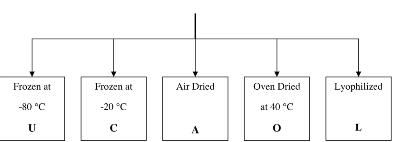
The effect of five sample pre-preatment procedures were considered in this work, i.e. frozen at -20 °C, frozen at -80 °C, air dried, oven dried at 40 °C and lyophilized. The sediment samples were formerly stored at -20 °C; they were thawed and homogenized, and then divided in five batches and subjected to the following drying conditions. Figure 2.1 summarizes the sample pre-treatment methodology. Further information of the different pre-treatments is given below:
Frozen Samples at -20 °C and -80 °C
Samples to be frozen were immediately transferred from the polyethylene container to individual capped glass sample holders, and the sample weight was recorded. The sediment contained in every sample holder corresponded to the whole sample intake either for mercury speciation or total mercury analysis. The samples labeled as C and U were stored at -20 °C and -80 °C, respectively. Samples were kept at these temperatures until analysis.
21 Air and Oven Dried Samples
These portions were first air dried during 72 h, and then they were grounded with an agate mortar and stored in polyethylene bottles. The remaining portions were dried for 48 h in an oven at 40 °C and then grounded with an agate mortar. In this work the air and oven dried sediments were tagged as A and O, respectively.
Lyophilized Samples:
Samples to be lyophilized (labelled as L) were first frozen at -80 °C and then lyophilized at 0,110 mBar for 18 h, after which they were ground in an agate mortar and stored in polyethylene bottles until analysis.
Figure 2.1 Sample pre-treatment scheme.
Sediment Samples
(Formerly frozen at -20 °C until analysis)
Frozen at -80 °C U Frozen at -20 °C C Air Dried A Oven Dried at 40 °C O Lyophilized L
22
2.1.3 Moisture and Major Components
The moisture content was determined separately by drying 1 g sample at 105 ± 2 °C to constant weight. From this, a correction to dry mass was obtained which was applied to all analytical concentrations reported.
The major element composition was determined by X-ray fluorescence spectroscopy; the samples were diluted (1:20) with lithium tetraborate and melted at 1350 C in a radio-frequency inductive oven to obtain 30 mm diameter pearls. The instrument was calibrated using 56 geological international reference samples.
Total C, H, N and S contents in the sediments were determined by elemental analysis using tin capsules and V2O5 as additive. The samples were combusted at 1000 °C and
analyzed by gas chromatography.
Organic carbon was determined by heating the samples at 300 °C in a sand bath and then at 550°C in an oven. The temperature of the oven was set first at 350 °C and then raised to 550°C by increments of 50 °C. The losses in weight were calculated and expressed in percentage.
Air dried samples were used for all the characterization tests.
2.1.4 Aqua Regia Mercury Extraction
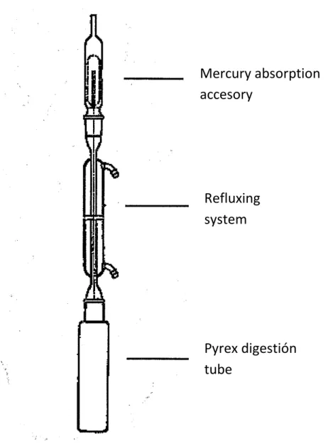
This aqua regia extraction procedure is based on the procedure recommended by the International Organisation for Standardisation (ISO) (21). To 1 g of sample weighed in 250 mL pyrex digestion tubes, 7 mL of 37% Hydrochloric Acid and 2,3 mL of 69% Nitric Acid were added (3:1 mixture). The sample was predigested at room temperature for 16 h with the refluxing system connected, and the mercury absorption accessory was filled with 15 mL of HCl 4% and then connected at the end of the reflux tube. Then, the suspension was digested at reflux conditions for 2 h at 130 °C in an aluminium block. Once cooled down, the acid in the mercury absorption accessory was transferred to the Pyrex tube, and the obtained suspension was filtered using an ash-less filter paper (Whatman no. 40), and its volume was made up to 50 mL by adding HCl 4%. These
23
solutions were transferred to polyethylene containers and stored at 4 °C until analysis. Blanks were measured in parallel for each batch using the reagents described above. Figure 2.2 shows the reflux system used for this digestion.
Figure 2.2. Reflux system for the determination of total mercury by the aqua regia digestion.
2.1.5 Microwave Mercury Extraction (EPA 3200)
This procedure involves the microwave assisted extraction of mercury species from soil or sediment samples by using a solution of 4,0 M HNO3 (21). The dried or wet
homogenized sediment is weighed (1,0 ± 0,2 g) into microwave extraction vessels, 10
24
mL of 4,0 M HNO3 was added to each sample, the microwave vessels were sealed and
then irradiated at 100 °C for 10 min. The vessels were allowed to cool and the extracts filtered through a whatman 40 filter. The extracts were stored at 4 °C until analysis. Blanks were measured in parallel for each batch using the reagents described above. This extraction procedure was carried out formerly with HCl 4,0 M instead of HNO3
due to the known quenching effect of the nitrogen in the detection signal, but after some tests it was determined that using HNO3 did not affect the fluorescence signal, and for
this reason the extractions were performed in the same conditions as stated in the standard.
2.1.6 Methyl, Ethyl and Inorganic Mercury Determination
The speciation of mercury was performed in the extracts obtained in the microwave assisted extraction by HPLC-UV-CVAFS. The separation of the compounds was achieved injecting 100 µL of sample, standard, mobile phase or blank into the liquid chromatograph. The mobile phase for the analysis of Hg2+ and MeHg+ was composed by MeOH:APDC pH 5,5 (1,5 mM APDC + 10 mM NH4Ac) in a ratio 80:20 as
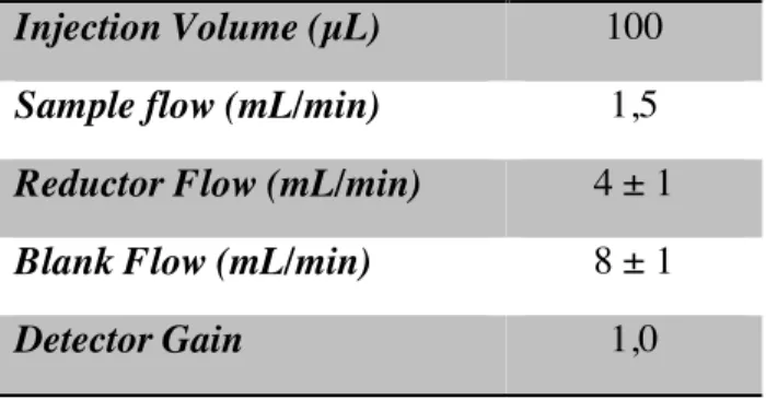
established in a previous work (22). In the case of the simultaneous analysis of Hg2+, MeHg+ and EtHg+ the mobile phase had the same composition but the ratio between the organic and aqueous phases was optimized in this work. In the reduction step, a solution of tin (II) chloride 1,5% in HCl 4% was used. The main experimental conditions are shown in the table 2.2.
Table 2.1. Experimental conditions for the mercury speciation analysis.
Injection Volume (µL) 100
Sample flow (mL/min) 1,5
Reductor Flow (mL/min) 4 ± 1
Blank Flow (mL/min) 8 ± 1
25
The data acquisition was done with the Pendragon® 1.0 software; peak area was integrated for making the calibration curves.
2.1.7 Total Mercury Determination
In the case of the total mercury determination, the sample, standard or blank are fed directly into the cold vapor generator and analyzed in the same way as the samples for speciation analysis, but the volume intake is 20 mL because the sample is continuously pumped until the detected signal is stabilized. The extracts from the microwave assisted extraction were oxidized before the analysis by adding 50 µL of a solution of BrO3-/Br
0,55%. The signal height was recorded with the software Avalon 1.1®.
2.1.8 Labware cleaning
All laboratory glassware and plasticware were rinsed three times in double deionised water after being soaked in a HNO3 (10%, v/v) bath overnight.
2.2 Instruments
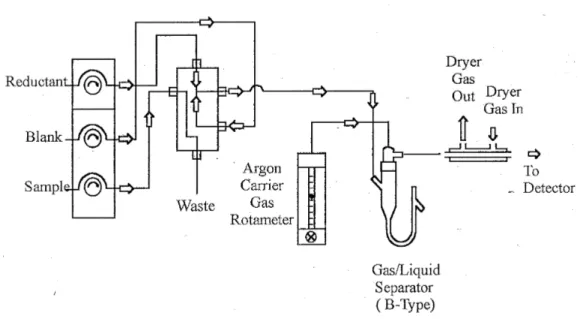
2.2.1 Description of the mercury analysis system
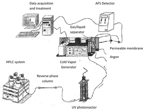
The speciation of mercury was performed by HPLC-UV-CVAFS (cold vapor generation atomic fluorescence spectrometry coupled to an online UV post-column oxidation system). A schematic diagram of the mercury chemical vapor generator system is reported in Fig. 2.3. The separation of the compounds was achieved injecting 100 µL of sample, standard, mobile phase or blank through a manual injector into the reversed phased column. The species were separated using a mobile phase composed of methanol: ammonium pyrrolidinedithiocarbamate (APDC) at pH 5,5. APDC is used as a complexing agent because with this reagent, highly stable and non-ionic complexes which are suitable for the reverse phase separation are formed with the Hg species.
26
Figure 2.3. Schematic diagram of the HPLC–UV-CVAFS system.
The separated species must be transformed into inorganic mercury because the CVAFS system is used for determining total inorganic mercury (Hg2+), so all the complexing forms present in the sample have to be converted to Hg2+.
In order to break the Hg-C bond in the organomercuric compounds, the species separated by HPLC are on-line oxidized under a photoreactor which consists in an ultraviolet lamp (UV) and a PTFE tube coiled around the lamp. The lamp generates 150 W of radiation at 250 nm. The lamp is inserted into a support on which a PTFE tube (0,5 mm diameter and 12 m long) is coiled. All the system is covered with an aluminium sheet to reflect the non absorbed radiation and to prevent the emission of the radiation outside the reactor. Hg2+ is obtained after passing the effluent of the column through the UV photoreactor
27
Elemental mercury (Hg0) is then formed by using acidified stannous chloride; the following is the redox reaction of the CV process:
Hg2+ + Sn2+ Hg0 + Sn4+
The separation of the elemental mercury generated after the reduction step is assisted by the introduction of an argon stream into the transference line. Latterly, the mixture of gas and aqueous fluxes is separated in a gas–liquid separator device. The elemental mercury is driven to the AFS detector by the Argon stream.
In the Cold Vapor Generation System and AFS Detector unit, the inorganic mercury is first reduced into the elemental form and then separated from the solution. The system consists of a constant speed multi-channel peristaltic pump (100 rpm) to deliver the tin chloride and sample solutions, an electronically controlled switching valve to alternate between blank and sample solutions, and a gas/liquid separator which isolates and delivers the gaseous products to an atom reservoir where subsequent spectroscopic determination takes place.
The flow pattern of the system is represented in figure 2.4. When activated, the unit progresses through a cycle involving four stages: Delay, rise, analysis and memory. Peak height is recorded during the analysis step while the other steps involve purge and cleaning.
28
The two liquid streams are mixed in the sample valve, where the reduction reaction takes place, the streams and all gaseous products are continuously pumped into the gas/liquid separator. The gaseous products, both elemental mercury and hydrogen are flushed from the gas/liquid separator by a stream of argon and carried through a connecting tube to the atomic florescence detector. The samples enter the detector as a gas, which is channeled through a chimney past a light source and a photomultiplier which are at right angles to each other (24).
The mercury vapor absorbs the radiation emitted at 254 nm from a Hg lamp, and fluoresces at its characteristic wavelength (254 nm). The photomultiplier detects the fluorescence from the sample.
2.2.2 Equipments
• HPLC System:
o Quaternary Pump Agilent 1100
o Manual Injector Rheodyne 7725i, Stainless Steel. o 100 µL Injection loop
o Chromatographic Column ODS Hypersil. Thermo. 250 x 4,6 mm. 5 µm particle diameter, 120 Å pore diameter
• Hydride generator PSA 10.004. P S Analytical LTD. • Ultraviolet lamp Heraeus TQ 150, 150W.
• Merlin Fluorescence Detector PSA 10.0023.
• Sequential XRF Spectrophotometer Phillips PW2400.
• Elemental Analyzer EA 1108 CHNS-O, Carlo Erba Instruments. • Spectrophotometrer ICP-OES Perkin Elmer Optima 3200 RL • Analytical Balance Mettler Toledo AB204 with 0,1 mg precision. • Balance AND EK-2000i with 0,1 g precision.
• Oven Memmert UPL-800. • Electronic pipettes:
o Rainin EDP3-Plus of 1000, 2000, 5000 and 10000 µL. o BIOHIT Proline, 50 – 1200 µL.
• pH meter Basic 20 Crison with pH 4 and 7 calibration standards • Magnetic stirrer SBS instruments A-06.
29
• Deionization system Sistema Eilx 3 - Milli-Q Gradient A10, Millipore.
2.2.3 Reagents and standards
The reagents and standards used in the experimental work are presented below.
2.2.3.1 Standards
• Inorganic Mercury 1000 mg/L: This standard was prepared from the HgCl2 salt
(pro analysis, ACS, min, 99,5%, Merck) in HNO3 1%. The final solution
contains 1000 mg/L of mercury as Hg2+. The standard was stored at 4 °C in a dark bottle.
• Methylmercury 1000 mg/L: Prepared by dissolution of CH3HgCl (Aldrich
Chem. Co.) in 3% MeOH. The final solution contains 1000 mg/L of mercury as Hg. The standard was stored at 4 °C in a dark bottle.
• Ethylmercury 1000 mg/L: Prepared by dissolution of CH3CH2HgCl (Aldrich
Chem. Co.) in 25% acetonitrile with agitation. The final solution contains 1000 mg/L of mercury as Hg. The standard was stored at 4 °C in a dark bottle.
2.2.3.2 Reagents
• Nitric acid (HNO3) 69%. HIPERPUR, Panreac.
• Hydrochloric acid (HCl) 35%. HIPERPUR, Panreac.
• Methanol. (CH3OH) HPLC gradient grade, PAI-ACS 99,9%, Panreac.
• Acetonitrile (CH3CN) HPLC gradient grade for LC, LiChrosolv 98,0%,
Merck.
• Acetic acid (CH3COOH) Glacial, TMA HIPERPUR, Panreac.
• Tin (II) chloride 2-hydrate (SnCl22H2O), PA-ACS, max. 0,000005% Hg,
Panreac.
• Ammonium acetate (CH3COONH4) grade reagent for analysis, Merck.
31
32
3.1 Analytical Methodology for Hg
2+, MeHg
+and EtHg
+determination
in waters
3.1.1 Optimisation of the mobile phase composition
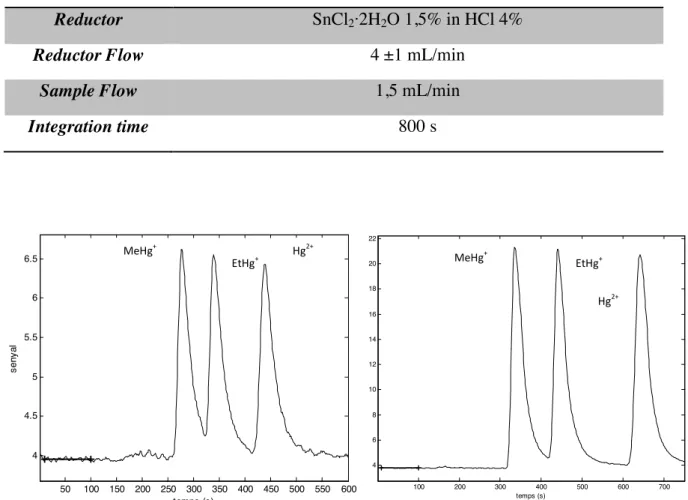
In an earlier work, a method for the speciation of Hg2+and MeHg+ by HPLC-UV-CVAFS was developed (22). In order to include the analysis of a third species, EtHg+, the first approach was to run standards under the same chromatographic conditions as established in the former work. The obtained chromatograms showed that those conditions did not allow the complete separation of the two organomercurial species. The figure 3.1.a shows that even at low concentrations (25 µg/L) the peaks of these compounds were not completely resolved. The resolution should be improved if the residence time of the species inside the columns is higher, which can be achieved by increasing the proportion of the aqueous component in the mobile phase i.e. reducing the elution power of the mobile phase. For this reason the proportion of APDC pH 5,5 was elevated from 20% to 25%. The obtained results are similar to the one appearing in the figure 3.1.b. The resolution of the MeHg+ and EtHg+ peaks was increased even at high concentrations (200 µg/L). Thus the mobile phase allowed the significant differences in chemical and physical characteristics of mercury species to be partly overcome and thus permitted the determination of widely differing compounds (inorganic mercury cations and strongly polar monoalkylmercury compounds like MeHg+ and EtHg+) in a single separation step (see chromatograms in Fig. 3.1). The experimental conditions for the separation appear in the table 3.1.
33
Table 3.1. Experimental conditions for the analytical speciation of Hg2+, MeHg+ and EtHg+.
Mobile Phase 75% MeOH – 25 % APDC 1,5 mM + NH4Ac 10 mM pH 5,5
Reductor SnCl22H2O 1,5% in HCl 4%
Reductor Flow 4 ±1 mL/min
Sample Flow 1,5 mL/min
Integration time 800 s
Figure 3.1. Separation of the mercury species with different mobile phase in proportions. (a) 80:20 (25 µg/L), (b) 75:25 (200 µg/L)
3.1.2 Establishment of the quality parameters
3.1.2.1 Calibration Curves
After determining the adequate mobile phase, several standards prepared in mobile phase were analyzed in order to determine the calibration curve and the linear range. The standards and blanks were analyzed and the calibration curve was obtained. The calibration parameters are given in the table 3.2.
100 200 300 400 500 600 700 4 6 8 10 12 14 16 18 20 22 temps (s) se n y a l 50 100 150 200 250 300 350 400 450 500 550 600 4 4.5 5 5.5 6 6.5 temps (s) se n ya l
34
Table 3.2 Regression parameters in the calibration curve for the speciation of mercury. a: slope, b: intercept and r2: correlation coefficient.
Regression Parameter Hg 2+ EtHg+ MeHg+ a / (µg/L)-1 2,1333 1,7416 2,1564 b 0,3655 -0,5562 1,4779 r2 0,9997 0,9992 0,9998
The method shows an adequate linearity (r2 > 0,999) in the range between 10 and 250 µg/L, and the method sensitivity is lower than the obtained when the speciation analysis is focused on Hg2+ and MeHg+ because for these analytes the slope is slightly lower in this study than the obtained in the previous one.
3.1.3 Detection and Quantification Limits
After establishing the adequate organic phase/aqueous phase ratio for the components of the mobile phase, the detection and quantification limits were determined. These quality parameters were established for the three studied species by injecting standard solutions of Hg2+, MeHg+ and EtHg+ of 5, 12.5, 25, 50, 100 and 250 µg/L in one experimental session.
The limit of detection (LOD) is defined as the analyte concentration which gives a signal equal to signal of the blank, yB, plus three times its standard deviation, sB. (25)
LOD = yB + 3sB.
In chromatographic techniques is not possible to determine the signal of the blank in the same way as for the standards and samples. For this reason is necessary to use the average of the signal recorded during the first 100 seconds of analysis (when no compounds are being eluted) as a measure of the obtained background response. To obtain the concentration in the limit of detection a calibration curve must be obtained
35
using net signal units instead of peak area. The table 3.3 shows the regression parameters for the three mercury species:
Table 3.3. Regression parameters for the determination of the LOD. a: slope, b: intercept and r2: correlation coefficient.
Compound a / (µg/L)-1 B r2
Hg2+ 0,0544 -0,1000 0,9983
MeHg+ 0,0582 -0,1101 0,9989
EtHg+ 0,0551 -0,3601 0,9965
In order to determine the standard deviation of the background signal (sB), 11
consecutive measurements of calibration standards in the low part of the calibration graph prepared in mobile phase were considered. The background standard deviation was 0,067 and a mean value of 3,675 was obtained. The concentration in the limit of detection is obtained applying the regression parameters to the mean background signal. The obtained concentrations in the limit of detection were obtained are 3,7, 3,5 and 3,7 µg/L for the Hg2+, MeHg+ and EtHg+ respectively.
The limit of quantification (LOQ) is estimated using the standard deviation of the background signal in a similar way as made for the LOD. LOQ is defined as the blank signal plus ten times its standard deviation. Consequently, the concentration in the limit of quantification (CLOQ) corresponds to ten times the background signaldivided by the
slope of the calibration curve (a). The slope of the calibration curve and the standard deviation of the background signal are the same appearing in the table 3.3. The CLOQ
value obtained was 12 µg/L for Hg2+, MeHg+ and EtHg+.
3.1.4 Recovery studies
In order to evaluate the method performance with real samples under reproducibility conditions, two water samples were spiked with a known concentration of the mercury species and analyzed in three different days. The samples selected for the recovery and accuracy study were a tap water sample and a commercial mineral water; these samples
36
were filtered through a 20 µm membrane and spiked with 20 µg/L of Hg2+, MeHg+ and EtHg+, which corresponds to a low concentration taking into account the LOQ of the method. The standards, blanks and samples were prepared and analyzed in three different days to meet the reproducibility conditions. The obtained results are summarized in the figure 3.2.
The three mercury species have different recoveries. The MeHg+ recovery is around 100% and the coefficient of variation (CV) below 10% for both tap and mineral water samples during the three experimental sessions. In the case of the inorganic mercury and EtHg+ an inverse behavior was found: Hg2+ has a recovery that is over 150% while the recovery for the EtHg+ is around 80%; the dispersion of the results is also higher than the obtained for the MeHg+. The figure 3.2 shows the overall behavior, and it is clear the yielding of high recoveries for Hg2+ and low recoveries for EtHg+ in a systematic way.
Figure 3.2. Recovery of the spiked mercury species in two different waters, a: Mineral water, b: Tap water. n=3, error bars correspond to standard deviation.
37
This behavior can be observed in a better way in figure 3.3. These chromatograms suggest that EtHg+ might be undergoing chemical reactions in these matrices resulting in the formation of Hg2+. The figure 3.3.a shows the behavior of the standards, where the peaks of the three mercury species have a comparable height and area, in 3.3.b and c. the reduction in the size of the EtHg+ peak and the increase in the Hg+ in the real samples is clear. For this reason, an additional set of experiments was carried out in order to ascertain if EtHg+ was getting converted into the inorganic species during the measurement sessions.
Figure 3.3. Obtained peaks in the determination of 20 µg/L MeHg+, EtHg+ and Hg2+ in three different water samples a: calibration standard, b: spiked mineral water, c: spiked tap water. 100 200 300 400 500 600 700 800 4.2 4.4 4.6 4.8 5 5.2 5.4 5.6 5.8 6 temps (s) se n ya l 100 200 300 400 500 600 700 800 4 4.5 5 5.5 6 6.5 7 temps (s) se n ya l 100 200 300 400 500 600 700 800 4 4.5 5 5.5 6 6.5 7 temps (s) se n ya l 100 200 300 400 500 600 700 800 4.2 4.4 4.6 4.8 5 5.2 5.4 5.6 5.8 6 temps (s) se n ya l 100 200 300 400 500 600 700 800 4 4.5 5 5.5 6 6.5 7 7.5 temps (s)
38
3.1.5 Stability studies for EtHg+
A series of experiments were performed in order to determine if the changes in the quantified concentrations of EtHg+ and Hg2+ for the spiked samples were due to the conversion of EtHg+ into Hg2+ or due to matrix interferences. Both water samples were spiked with 20 µg/L of MeHg+, EtHg+ and Hg2+, mixtures of two compounds EtHg+/Hg2+, MeHg+/EtHg+ and EtHg+ alone. The samples were first injected as soon as prepared and then at fixed elapsed times, to control the evolution of the chomatographic peaks. The obtained results appear in the figure 3.3. From the figure 3.3.a it can be seen that a standard solution prepared in double deoinised water does not present any alteration in the peaks and the three compounds are detected with similar intensity.
The figures 3.3.b and c demonstrate the degradation of EtHg+ in the tap water sample. The first chromatogram was recorded after spiking the sample with the three species, and the Hg2+ peak looks increased when compared to the other peaks, the gradual increasing of the Hg2+ peak is evident. In a similar way, the mixtures composed by EtHg+ and other specie show that the same phenomenon occurs even when the sample is not fortified with three species simultaneously, chromatogram 3.3.c evidence the formation of Hg2+ out of EtHg+ after 24 hours.
Chromatogram d is obtained after spiking the mineral water with a mixture of the three species, is clear that EtHg+ and Hg2+ have similar peak area. After 24 h the Hg2+ peak shows a slight increase in the height, but it can’t be considered as evidence of conversion from EtHg+ to Hg2+ because the EtHg+ peak does not decrease. Neither the mixtures of two species or for samples injected with only EtHg+ showed a marked change in the peak height. Figures 3.3.e shows the overlapped peaks of EtHg+ at three different times, and no evidence of formation of Hg2+ is observed after 24 h. A chemical reaction between the matrix components and the mercury species can’t be proved for mineral water.
39
Figure 3.3. Obtained chromatograms in the speciation analysis of mercury in waters. a: Calibration standard of MeHg+, EtHg+ and Hg2+; b: Tap water spiked with MeHg+,
EtHg+ and Hg2+; c: Tap water spiked with EtHg+; d: Mineral water spiked with MeHg+, EtHg+ and Hg2+; e: Mineral water spiked with, EtHg+. All the solutions are 20 µg/L.
0 100 200 300 400 500 600 700 3 3.5 4 4.5 5 5.5 6 time (s) Si g n a l 0 100 200 300 400 500 600 700 3 3.5 4 4.5 5 5.5 6 time (s) Si g n a l 0 100 200 300 400 500 600 700 3 3.2 3.4 3.6 3.8 4 4.2 4.4 4.6 4.8 time (s) Si g n a l 0 100 200 300 400 500 600 700 3 3.2 3.4 3.6 3.8 4 4.2 4.4 4.6 4.8 time (s) Si g n a l 0 100 200 300 400 500 600 700 3.2 3.4 3.6 3.8 4 4.2 4.4 time (s) Si g n a l 0 100 200 300 400 500 600 700 3.2 3.4 3.6 3.8 4 4.2 4.4 time (s) Si g n a l 0 100 200 300 400 500 600 700 3 3.2 3.4 3.6 3.8 4 4.2 4.4 4.6 time (s) si g n a l 0 100 200 300 400 500 600 700 3 3.2 3.4 3.6 3.8 4 4.2 4.4 4.6 time (s) si g n a l 0 100 200 300 400 500 600 700 3 3.2 3.4 3.6 3.8 4 4.2 4.4 4.6 time (s) si g n a l 0 100 200 300 400 500 600 700 3.6 3.8 4 4.2 4.4 4.6 4.8 time (s) Si g n a l 0 100 200 300 400 500 600 700 3.6 3.8 4 4.2 4.4 4.6 4.8 time (s) Si g n a l
40
3.2 Analytical especiation of mercury in sediments: Effect of sample
pre-treatment
The main aim of this work was to determine the influence of the sample pre-treatment in the determination of total mercury and mercury speciation in sediments. With the aim of selecting the sediment samples to be studied, total mercury analysis was performed on samples from the Venice canal and Barcelona Harbor used in the research group for other studies. The samples in more quantity and with a level of total mercury suitable for the detection capability of the method were preferred. For this reason, two polluted sediments samples (St. 7 and St.12) were subjected to five different sample pre-treatments: freezing at -80 and -20, air drying, oven drying and lyophilizing. Details regarding the pre-treatment procedures are given in section 2.1.2.
3.2.1 Sample Characterization
In order to determine the composition of the two studied sediments, the characterization of the sediments in terms of moisture content, elemental analysis (N, C, H, S), major elements by XRF and losses on ignition (LOI) at 550 °C expressed as percentage were performed by duplicate.
The elemental composition, losses at 550 °C and the major elements are showed in the table 3.4 (mean values and standard deviation). The values found in the sediments were comparable to those obtained in previous studies for samples collected in the same zone (19). The high levels of total carbon and losses at 550 °C found might suggest an elevated contamination of the sediments due to anthropogenic pollution. As is expected, the samples have a similar composition, but the sample St. 7 has a higher level of N, C, and P which likely indicates a mayor level of anthropogenic activity.
41
Table 3.4 Elemental composition and mayor components for the sediment samples.
St. 7 (%) St. 12 (%) N 0,48 ± 0,04 0,21 ± 0,01 C 11 ± 0,2 7,9 ± 0,2 H 1,08 ± 0,06 0,41 ± 0,05 S 0,99 ± 0,06 0,86 ± 0,05 Fe2O3 3,45 ± 0,05 3,29 ± 0,01 MnO 0,05 ± 0,01 0,05 TiO2 0,37 ± 0,01 0,36 ± 0,01 CaO 15,8 ± 0,1 18,54 ± 0,01 K2O 1,70 ± 0,03 1,66 ± 0,01 P2O5 0,40 0,17 SiO2 28,5 ± 0,2 28,9 ± 0,1 Al2O3 7,77 ± 0,08 7,4 ± 0,2 MgO 7,4 8,4 ± 0,7 Na2O 2,47 ± 0,04 1,84 ± 0,05 Losses at 550°C 25 ± 1 16 ± 3
In the table 3.5 the humidity of the samples is showed, where it can be seen that after applying the three drying procedures the samples remain with a similar amount of final moisture. In the case of the frozen samples the water content is higher because these samples were taken just after the thawing and homogenization of the sediments. The moisture values were used to report the mercury concentration in a dry basis.
42 Table 3.5 Sample characterization: Moist content
Treatment St. 7 St. 12 Humidity (%) Air Dried 2,6 2,0 Oven Dried 1,8 1,3 Lyophilized 2,2 1,5 Freezed (-20°C) 50,4 38,9 Freezed (-80°C) 50,2 38,4
3.2.2 Comparison of Different Sample Pre-treatment Procedures
Total mercury concentration was determined in both sediments by CVAFS after an aqua regia extraction. The speciation analysis was performed by a microwave assisted (MW) extraction and a further determination following the procedure (section 2.1.4) by HPLC-UV-CVAFS. As an intended analytical control check, total mercury content in MW extracts was determined by CVAFS after oxidation with a BrO3-/Br- solution to obtain the sum of all the possible mercury species present in the extracts.
The reference material IAEA-405: for trace elements and methylmercury in estuarine sediment, certified for total mercury (0,81 ± 0,04 mg/Kg) and methylmercury (5,49 ± 0,53 µg/Kg), from the International Atomic Energy Agency (26), was used for quality control purposes.
The level of total mercury found depends on the kind of pre-treatment applied. In the figure 3.4, for both samples it is clear that when a frozen sample is analyzed, the measured value of total mercury (aqua regia extracts) is lower than the obtained when the sample is dried. One possible reason for this behavior is the high level of water in the frozen samples, which can partially dilute the mixture of acids and make the extraction less effective. This fact was pointed out by other researchers in previous works (13). Another reason could be connected to the difficulty of handling wet samples
43
that might cause the incomplete transfer of the sediment from the sample holder to the Pyrex tube where the digestion is performed, resulting in potential sample losses during the process.
Figure 3.4. Aqua regia total mercury in two sediment samples. A: Air dryed, O: Oven Dried, L: Lyophilized, C: frozen at -20 °C, U: Frozen at -80 °C. Error bars correspond to s.d. of 3 measurements
From the speciation analysis it was found that only the inorganic mercury was present in detectable amounts, MeHg+ was below the detection limit, regardless the sample pretreatment; this result makes sense taking into account the low methylmercury concentration in the sediments (around 1% of the total Hg) (27,28). Figure 3.5 shows typical chromatogram obtained for the sediment samples. In the case of the sample St.7, the level of Hg2+ was similar regardless the pre-treatment. When comparing the Hg2+ concentration with the mercury concentration obtained after analyzing the oxidized speciation extracts, is clear that the latter is surprisingly higher than the Hg2+ concentration. This result suggests that might be some mercury species in the extract which are not detected in the speciation analysis but are detected as Hg2+ after the oxidation step. This result was not repeated for the sample St. 12, where both the speciation and the total mercury levels are similar for the microwave extracts, which is the expected behavior. In the figure 3.6 the mercury concentration found in the MW extracts can be observed.
44 50 100 150 200 250 300 350 400 450 500 550 600 4 4.5 5 5.5 6 6.5 7 time(s) Si g n a l
Figure 3.5 Chromatogram for the speciation analysis of the sample St. 7.
Figure 3.6. Comparison of different sample pre-treatments. a: Sample St. 7, b: Sample St. 12. Oxidized extracts: Total mercury in the MW extract. Speciation: Hg2+ mercury in the sediment samples.
45
When comparing the mercury concentration obtained in the microwave extracts with the total mercury obtained by the aqua regia method it can be seen that for both samples the Hg2+ is lower than the total mercury. The recovery from the aqua regia total mercury was around 80% for all the dried sediments, and for the frozen samples the recovery was higher due to the lower value of the total mercury concentration.
The method accuracy was checked by analyzing the standard reference material IAEA-405, estuarine sediment. As expected according to the LOD of the used method, only Hg2+ was detected in the CRM in the speciation analysis. The obtained total concentration was 1,02 ± 0,03 mg/Kg (mean ± standard deviation of two measurements) . Significant differences were found between the certified value and the one provided by the acid leaching method at 95% confidence level. The mercury recovery is around 126 %, this result implies a lack of accuracy in the method that must be overcome in further studies.
According to the obtained results (figure 3.6.), it can be observed that the total mercury content is in agreement with the reported in previous works (19). Tthe sample St. 7 has a higher level of mercury which is around 8 mg/Kg while the sample St.12 has a concentration around 2,4 mg/Kg.
To determine whether or not mercury concentration changed significantly among the different sample pre-treatments, a one-way analysis of variance (ANOVA) test was performed. The results are given in the table 3.6 and clearly show that depending upon the chosen pre-treatment strategy there will be significant differences in the mercury concentration. The only exception was the Hg2+ in the sample St.7, where the obtained F value was lower than the Fc for a 95% confidence level, and this means that regardless the selected sample pretreatment the obtained Hg2+ concentration will be statistically equivalent.
46
Table 3.6 One way ANOVA analysis for the five sample pre-treatment procedures (P = 0,05). F Fc Significant Differences St. 7 Aqua Regia 7,37 3,48 Yes Microwave 4,35 Yes Speciation 1,89 No St. 12 Aqua Regia 5,6 3,63 Yes Microwave 12,0 Yes Speciation 10,3 Yes
Considering that samples subjected to drying show a similar behavior for both total mercury and speciation analysis, another ANOVA was performed to determine if the air dried, oven dried and lyophilized samples yield an equivalent concentration of mercury.
Table 3.7 One way ANOVA analysis for three sample pre-treatment procedures: Air drying, oven drying and lyophilizing (P = 0,05).
F Fc Significant Differences St. 7 Aqua Regia 0,45 5,14 No Microwave 0,07 No Speciation 1,06 No St. 12 Aqua Regia 0,87 No Microwave 5,62 Yes Speciation 9,85 Yes
From the table 3.7 according to the ANOVA test, is evident that in the case of the sample St. 7 there are no significant differences among these three sample
pre-47
treatments, it doesn’t matter the pre-treatment of choice because the total mercury and the Hg2+ measured in these samples is equivalent. This founding is not corroborated in the sample St. 12, where the concentrations determined in the microwave extract (both total mercury and Hg2+) will vary from one pretreatment to another. The study on the effect of sample pre-treatment must be extended to other sediments of different origins.
3.2.3 Effect of sample pre-treatment on heavy metal determination.
The concentration of Cu, Cr, Ni, Pb and Zn in the aqua regia extracts was determined by ICP-OES, for each pre-treatment one sample was analyzed. Results appear in the table 3.8. The concentrations are in accordance with the representative values for the zone. In order to determine if there is any evidence that may suggest significant differences in the heavy metal content among the sediment samples, a Dixon's Q-test for the detection of single outliers was performed. For both samples the presence of outliers was detected at the chosen level of significance ( = 0,05). For the sample St. 7, results obtained for Zn and Ni in the air dried sample were outliers, while in the sample St. 12, the results detected are those from lyophilized samples for Zn and Cr.
This result might suggest the no equivalence of the total concentration of some heavy metals among samples treated in different ways, but is not enough evidence to assure that results vary significantly.
48
Table 3.8. Heavy metal concentration in aqua regia extracts for samples subjected to different pre-treatments. A: Air dryed, O: Oven Dried, L: Lyophilized, C: frozen at -20 °C, U: Frozen at -80 °C. Cu (mg/Kg) Cr (mg/Kg) Ni (mg/Kg) Pb (mg/Kg) Zn (mg/Kg) St. 7 A7 198 37,1 24,8 135 860 L7 181 32,6 23,9 166 793 O7 209 35,8 26,9 140 853 U7 197 36,4 26,8 133 880 C7 203 36,7 26,4 143 860 St.12 A12 104 26,1 18,9 66,9 439 L12 111 25,6 21,4 73,1 456 O12 108 26,7 22,2 64,2 455 U12 108 26,8 22,1 67,1 459 C12 108 26,3 21,6 68,8 455
49
CONCLUSIONS
• The separation of Hg2+, MeHg+ and EtHg+ by the HPLC-UV-CVAFS hyphenated technique in waters was achieved. This speciation analysis was done using a reverse phase column (C18), with a mobile phase composed of (75:25)
MeOH – water containing APDC 0,0015M as complexing agent and HN4Ac
0,01M at pH 5,5. The obtained detection and quantification limits make the method applicable in the determination of these species in environmental samples with a medium-high level of pollution. In order to achieve detection limits suitable for the usual levels of mercury in non-polluted samples is necessary to further develop preconcentration strategies like solid phase extraction.
• Degradation of EtHg+ into Hg2+ in fortified tap water samples was verified. This phenomenon makes not possible the evaluation of the accuracy in the determination of Hg2+, MeHg+ and EtHg+ in such kind of samples until the reason and consequences of the EtHg+ decomposition is well understood.
• When analyzing total mercury in sediments a drying step for sample pre-treatment is recommended (air drying, oven drying at 40 °C or lyophilization). Determining the total content of mercury in the samples after keeping the sediments at -80 and -20 °C yield a lower mercury concentration than the obtained when samples are analyzed after drying.
• Significant differences in the content of Hg2+ in sediment samples subjected to five pre-treatments were found. As no CRM is available for the Hg2+ content in sediments, the preferred pretreatment procedure cannot be established. For the two studied sediments, procedures implying sample drying provided the best results. Among these pre-treatments, air drying and oven drying at 40°C are preferred due to their execution simplicity.
51
REFERENCES
1. Office of Air Quality Planning & Standards and Office of Research and Development. (1997). Volume V: Health Effects of Mercury and Mercury Compounds. Mercury Study Re|port to Congress. EPA.
2. Repetto, R. Reppeto, G. (2000). Metales. In: Manual de Toxicología. Madrid: Básica. Ediciones Díaz de Santos, S. A. 619-649.
3. Who Air Quality Guidelines - Second Edition Chapter 6.9 Mercury
4. Žižek, S. Horvat, M. Gibiar, D. Fajon, V. Toman, M. (2007). Bioaccumulation of mercury in benthic communities of a river ecosystem affected by mercury mining. Science of the Total Environment. 377. 407–415
5. Sweet, L. Zelikoff, T. (2001). Toxicology and Immunotoxicology of Mercury: A Comparative Review In Fish And Humans. Journal of Toxicology and
Environmental Health, Part B, 4:161–205.
6. Programa de las Naciones Unidas para el Medio Ambiente Evaluación Mundial Sobre Mercurio. (2005). 41-44.
7. Time Network, Natural Resources Canada, The Mining Association of Canada and Environment Canada. (2002). Literature Review of Environmental Toxicity of Mercury, Cadmium, Selenium and Antimony in Metal Mining Effluents.
8. Jin Qian. (2001). Doctoral thesis Swedish University of Agricultural Sciences. 9. More, F. Kraepiel, A. Amyot, M. (1998). The Chemical Cycle and Bioaccumulation
of Mercury. Annu. Rev. Ecol. Syst. 29:543–66
10. Szpunar, J. Bouyssiere, B. Lobinski, R. Chapter 2: Sample preparation techniques for elemental speciation studies
11. Leermakers, M. Baeyens, W. Quevauviller, P. Horvat, M. (2005). Mercury in environmental samples: Speciation, artifacts and validation. Trends in Analytical Chemistry. Vol. 24, No. 5. 383-393.
12. Horvat, M. Bloom. N. Liang. L. (1993). Comparison of distillation with other current isolation methods for the determination of methyl mercury compounds in low level environmental samples. Part 1. Sediments. Analytucal Chimica Acta, 281:135 -152.