Random array of drifting acoustic receivers (RADAR'07)

(1)

CINTAL - Centro de Investiga¸

c˜

ao Tecnol´

ogica do Algarve

Universidade do Algarve

Random Array of Drifting Acoustic Receivers

(RADAR’07)

C. Soares, S. M. Jesus, P. Hursky, T. Folegot,

C. Martins, F. Zabel, L. Quaresma,

Dong-Shan Ko and E. F. Coelho

Rep 04/07 - SiPLAB 15/December/2007

University of Algarve tel: +351-289800131

Campus de Gambelas fax: +351-289864258

8005-139, Faro [email protected]

(2)

8005-139 Faro, Portugal

Tel: +351-289800131, [email protected] Laboratory performing SiPLAB - Signal Processing Laboratory

the work Universidade do Algarve, FCT, Campus de Gambelas, 8005-139 Faro, Portugal

tel: +351-289800949, fax: +351-289800066 [email protected], www.ualg.pt/siplab Projects RADAR (POCTI/CTA/47719/2002)

UAB (POCI/MAR/59008/2004)

Title Random Array of Drifting Acoustic Receivers 2007 (RADAR07): Acoustic Oceanographic Buoy Data

Authors C. Soares, S.M. Jesus, T. Folegot, C. Martins and F. Zabel Date December 15, 2007

Reference 04/07 - SiPLAB Number of pages 84 (eighty four)

Abstract This report describes the complete set of data acquired during the RADAR’07 sea trial, that took place aboard the NRP D. Carlos from July 9 - 15, 2007, off the west coast of Portugal, in the Set´ubal area. Clearance level UNCLASSIFIED

Distribution list IH(1), NURC(1), HLS(1), NRL(1), SiPLAB(2), CINTAL (1) Attached RADAR07 DVD (1 unit)

Total number of copies 7 (seven)

Copyright Cintal@2007

Approved for publication

S. M. Jesus General Director

(3)

III

Foreword and Acknowledgment

This report presents the data acquired with two Acoustic Oceanographic Buoy (AOB) systems and the preliminary results obtained during the RADAR’07 sea trial. The RADAR’07 sea trial took place off the west coast of Portugal in the Set´ubal area, during the period July 9 - 15, 2007.

The authors of this report would like to thank:

all the personnel involved, including NRP D. Carlos I crew;

the support from the involved institutions: Instituto Hidrogr´afico (IH), NATO Un-dersea Research Centre (NURC), Naval Research Laboratory (NRL) and Heat Light and Sound Research (HLS);

FCT (Portugal) for the funding provided under projects UAB (POCI/MAR/59008/2004) and RADAR (POCTI/CTA/47719/2002).

(4)

(5)

List of Figures

1.1 RADAR’07 working area location. . . 14 2.1 RADAR experiment area off the west coast of Portugal in the continental

platform in front of the Tr´oia Peninsula: transects A-B,C,D and E. . . 17 2.2 CTD locations performed by NRP D. Carlos I during RADAR’07. . . 19 2.3 recorded CTD casts from NRP D. Carlos I between July 9 and July 14,

2007: temperature profiles (a) and salinity profiles (b). The black thick curve is the mean profile. . . 19 2.4 RADAR’07 bathymetry map with thermistor strings’, ADCPs’, and SLIVA’s

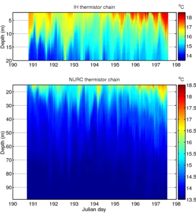
locations. SLIVA was deployed at point A. . . 20 2.5 Temperature data collected with the IH and NURC thermistor strings

cov-ering the whole duration of the RADAR’07 sea trial. . . 21 2.6 AOB22 thermistor string data for deployment days 192, 193, 194 and 195. 22 2.7 all CTD data upto 120 m depth (a) first three EOF’s computed from CTD

data up to 100 m depth (b). . . 23 2.8 Currents measured with the IH ADCP: Absolute current values (a);

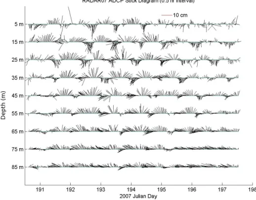
North-South component (b); East-West component (c). The blank portions denote depth and times where there is no data. . . 24 2.9 Currents measured with the NURC ADCP represented by a stick diagram.

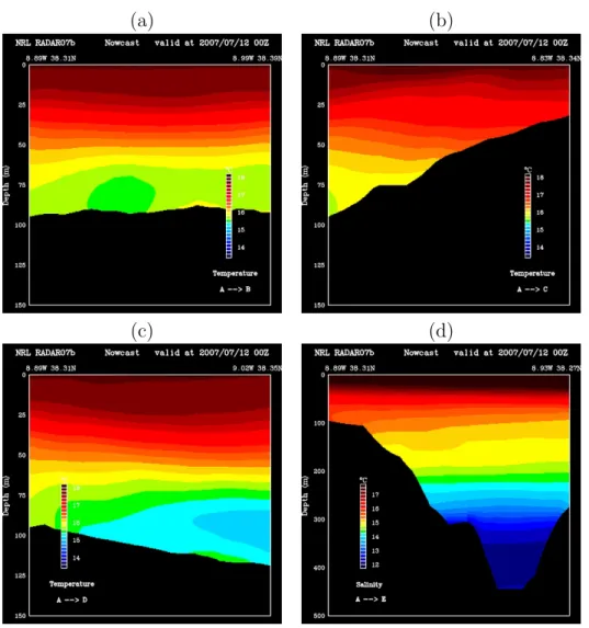
The sticks indicate current amplitude and direction. . . 25 2.10 Cross-section temperature predictions over cross-section A-B (a); A-C (b);

A-D (c); and A-E (d). . . 26 2.11 Surface temperature predition (a) and 50 m depth temperature prediction

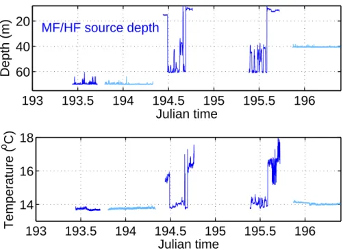
(b). . . 26 2.12 MF/HF source depth (upper plot) and temperature (lower plot) recordings.

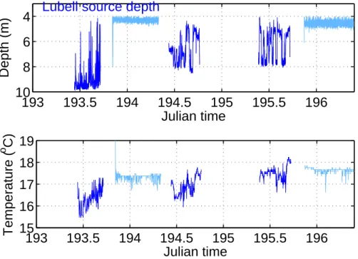
Lightblue color indicates intervals after AOBs recovery. . . 27 2.13 LF Lubell source depth (upper plot) and temperature (lower plot)

record-ings during deployments of Julian days 193, 194 and 195. Lightblue color indicates intervals after AOBs’ recovery. . . 28

(8)

2.14 Array depth oscillations, (a) and (b), and temperature recordings (c) and (d), through time for AOB21 (left) and for AOB22 (right). . . 29 2.15 GPS estimated AOB21 and AOB22 drift, NRP D. Carlos I tracks during

day 192 (a); GPS estimated AOB21 and AOB22 range from NRP D. Carlos I during day 192 (b); GPS estimated AOBs’ drift velocity during day 192 (c). . . 30 2.16 GPS estimated AOB21 and AOB22 drift, NRP D. Carlos I tracks during

day 195 (a); GPS estimated AOB21 and AOB22 range from NRP D. Carlos I during day 195 (b); GPS estimated AOBs’ drift velocity during day 195 (c). . . 33 3.1 Transmit voltage response for the low frequency Lubell 1424HP acoustic

projector. . . 37 3.2 Transmit voltage response for the high frequency ITC-1007 acoustic

pro-jector (a) and the medium frequency Neptune T170 acoustic propro-jector (b). 38 3.3 Spectrograms of the sequence emitted for the network tomograpgy

experi-ments: first and second frames (a); third and fourth frames (b). . . 39 3.4 Schematic illustrating of the NURC signal sequence . . . 42 3.5 Acoustic Oceanographic Buoy - version 2: receiving array hydrophone (a)

and surface buoy structure (b). . . 49 3.6 Spectrograms of signals received at receiver #4 of AOB22 during Drift

1: NURC signals received at approximately 2.4 km from the emitter (a); UALG LF and NURC HF tomography waveforms received at approxi-mately 2.0 km from the emitter. . . 52 3.7 Spectrograms of signals received at receiver #4 of AOB22 during Drift 2

at approximately 1.7 km from the emitter. . . 53 3.8 Spectrograms of signals received at receiver #4 of AOB22 during Drift 3

at approximately 1.4 km from the emitter. . . 54 3.9 Spectrograms of signals received at receiver #4 of AOB22 during Drift 4

at approximately 1.7 km from the emitter. . . 56 3.10 Envelope of the pulse compressed LFM chirps in the band 4000 to 8000 Hz. 57 3.11 Aligned envelopes of the pulse compressed LFM chirps in the band 4000 to

(9)

LIST OF FIGURES IX 3.12 Correlation time of pulse compressed LFM chirps in the band 4000 to

8000 Hz: MF band in black; HF band in gray. . . 58 4.1 Simplified scheme describing the local network set up on NRV D. Carlos I

during the RADAR’07 sea trial. . . 60 4.2 Baseline environmental model used for environmental inversion. . . 61 4.3 Baseline environmental model used for environmental inversion. . . 62

(10)

(11)

Abstract

The project “Random Array of Drifting Acoustic Receivers” (RADAR) started in 2004 with the objective of developing a network of drifting acoustic-oceanographic buoys (AOBs) for ocean observation. During this project a receiving buoy prototype was developed and tested at sea in 2005 (MakaiEx). During 2006 a second prototype was produced for im-plementing the network tomography concept, tested at sea during April/May 2007 in the MREA/BP’07 and now in the RADAR’07 sea trial from 9 to 15 July. The conceptual idea is to explore the spatially coherent capabilities of a series of vertical arrays at known positions and its ability to resolve the 3D temperature field along time both with known active sources and possibly with sources of opportunity. The slow movement of the re-ceivers with time, uncertainty of source - rere-ceivers relative geometry and evolution through a potentially poorly known bathymetry are the main challenges faced by the inversion of the acoustic data for environmental parameters. Another requirement is that acoustic inversion should be made in nearly real time, or at least, in a time compatible with the evolution of ocean parameters being monitored. The RADAR’07 took place from 9 to 15 July, 2007, in the continental platform, off the west coast of Portugal near the town of Set´ubal, approximately 50 km south from Lisbon and involved the oceanographic ship NRP D. Carlos I, from the Portuguese Navy. The data collected included an extensive CTD survey for ocean circulation modelling, acoustic data covering a wide band from 500 Hz up to 15 kHz, received on the AOBs and on a slim vertical array (SLIVA) and used for network tomography as well as for high-frequency tomography and underwater acoustic communications.

(12)

(13)

Chapter 1 Introduction

In todays life we are surrounded by networks: a computer network, a wireless network, a mobile phone network, etc... Actually we feel like being ourselves part of a huge World Wide network! The tendency is that the same networking concept will eventually extend to the ocean, with the objectives of ocean monitoring, exploration and surveillance. There are a number of such initiatives both in Europe (ESONET1_{), North America (Neptune}

and Orion2_{) and Japan (JAMSTEC)}3_{. These are large organizations that have a number}

of short and long term goals among which: i) obtain long time series of oceanographi-cal, biological and geophysical relevant parameters at selected locations, ii) be able to monitor those parameters on real (or near) real time and iii) correlated observed features from one location to the other to infer wide scale effects such as global warming, ocean circulation, internal tide effects, etc...and this should be done on real time and acces-sible from anywhere through the internet. So the ultimate goal is to have light, easily deployable systems that record, process and transmit environmental information to land stations for worldwide diffusion to authorized users. The concept proposed and developed under RADAR is to use a field of sonobuoys deployed by ship or aircraft to acoustically remote sense the environmental properties (watercolumn and seafloor) of a given ocean volume for Rapid Environmental Assessment (REA). The acoustic data or environmental data collected at the buoy is telemetered to a processing platform aiming at producing acoustic inversions. The resulting environmental models are integrated with concurrent oceanographic prediction models for nowcasts and forecasts in the given area.

These ideias as well as the hardware and algorithmic requirements for their implemen-tation formed the main objectives of the Acoustic Oceanographic Buoy Joint Research Project (AOB-JRP) launched in 2004 and involving various institutions 4 for a 3 year period. Under this JRP, the Signal Processing Laboratory (SiPLAB) team of the UALG has developed a first prototype version of the AO Buoy - AOB1 - in 2003 [1] and a second version - AOB2 - in 2005 [2]. At various levels of participation among partners, two sea trials took place under this JRP, both organized by NURC, the Maritime Rapid Environ-mental Assessment (MREA) 2003, in the North Elba area (Italy) [3] and the MREA’04 sea trial off the west coast of Portugal, in the continental platform near the town of Set´ubal [4]. During both sea trials the AOB1 was tested and the data gathered was analysed

1_{see web site www.esonet.org.}

2_{see website http://www.neptune.washington.edu/} 3_{see website http://www.jamstec.go.jp/}

4_{participating institutions: Universit´}_{e Libre de Bruxelles (ULB), Universidade do Algarve (UALG),}

Instituto Hidrogr´afico (IH), Royal Netherlands Navy College (RNLNC) and the NATO Undersea Research Centre (NURC).

(14)

Figure 1.1: RADAR’07 working area location.

and results are still being produced and published [5, 6, 7, 8, 9, 10, 11, 12]. AOB2 was first tested during the MakaiEx’05 in the Pacific in the framework of the High Frequency Initiative (HFi) both in high frequency tomography and underwater communications. In 2006 a second unit of the AOB was constructed in order to obtain a network with two nodes. During the RADAR’06 sea trial both of the buoys failed to acquire useful acoustic data for different reasons. Finally, during 2007 both AOBs were successfully deployed in two occasions, one during the MREA/Battle Preparation’07 sea trial, which took place in the Tyrrhenian Sea in April, and during the RADAR’07 aiming at collecting acoustic data with a minimal network of two acoustic receiving devices.

The RADAR’07 sea trial was jointly organized by CINTAL/SiPLAB and Instituto Hidrogr´afico (IH) with the collaborations of two other teams that were onboard the RV NRP D. Carlos I - from NURC (La Spezia, Italy) and HLS Reasearch, Inc. (San Diego, USA), and a team from the Navy Research Laboratory (NRL) that was responsible for running oceanographic predictions for the experimental area. This sea trial took place in the vicinity of Set´ubal in a site located approximately 50 km south of Lisbon, in Portugal, as indicated by the gray box in Fig. 1.1. It served the purpose of collecting acoustic and oceongraphic data for several scientific purposes: (a) low frequency acoustic data (up to

(15)

15 3 kHz) with multiple acoustic receiver arrays in order to support the RADAR project (POCTI/CTA/47719/2002) activities, in particular for fulfilling and supporting tasks 3 and 4; (b) high frequency acoustic data (up to 15 kHz) in order to support the devel-opment of a high frequency oceanic tomography concept; (c) to support an underwater communications concept using multiple acoustic receiver arrays; (d) oceanographic data to support ocean circulation modelling. Objective (a) closely follows under the steps of the previous line of the MREA experiments. Besides using multiple acoustic arrays, this sea trial provided an opportunity to test an online inversion software able to download data via wireless from the AOBs, extract the signals of interest, and perform environmen-tal inversion. The development of an operational processing platform is a component of paramount importance in the Acoustic REA concept. Objective (b) comes in line with the High Frequency Initiative and the MakaiEx’05 experiment, aiming at testing a high frequency tomography in an area with significant internal wave activity. The NURC team used a slim vertical array (SLIVA) designed for the reception of high frequency acoustic signals. This sea trial was particularly rich in terms of transmitted signals, as waveforms generated for the different objectives were simultaneously transmitted, either by superpo-sition of different waveforms in the same acoustic source, or by simultaneous deployment of two acoustic sources. This resulted in a highly productive sea trial for all teams on board.

During the RADAR’07 sea trial also extensive concurrent oceanographic measurements were performed with a CTD, ADCPs, moored thermistor strings, and a thermistor string colocated with one of the AOB arrays.

The present document aims at providing as much as possible a complete report of the various data sets acquired during the RADAR’07 sea trial both for acoustic and non-acoustic data as well as accompanying relevant information such as ship’s and buoys’ position, currents, temperature profiles, geo-acoustic information and other concurrent remote sensing data. The companion DVD contains all the basic data and respective master routines for data manipulation and pre-processing. This report is organized as follows: chapter 2 reports on all the non-acoustic data such as environmental data ge-ometries of intruments during the RADAR’07 sea trial; chapter 3 is dedicated to the acoustic data describing the instrumentation used to transmit and collect signals, and de-scribes transmission schedules throughout the experiment; chapter 4 briefly dede-scribes the computational facilities available on board, and reports on the inversion of acoustic data inversions carried out during the sea trial; finally section 5 concludes this report giving some hints about most interesting sets for posterior processing. Additionally, appendix sections were describing in detail files and routines used to generate waveforms included in the different transmission lineups composed for the sea trial.

(16)

The RADAR’07 sea trial

2.1 Generalities and sea trial area

The selected area for the RADAR’07 sea trial is shown in figure 2.1 together with the transects A-B, A-C, A-D, A-E planned for acoustic transmissions and geophysical obser-vations. There a number of interesting features in this area for performing shallow water experiments: in a small area within 10 km it encompasses a large range-independent plat-form at 120 m depth, a slowly range-dependent variable bottom to the coast, a highly range-dependent bottom to offshore, and a huge submarine depression on the continental platform: the submarine canyon of Set´ubal; it is an area with a known and well documented internal wave activity [13] and therefore potential generator of oceanographic -acoustic relevant features; logistically convenient for its vicinity to the base port of Lisboa and last, but not least, well protected from north winds and sea waves by the Espichel Cape (see general view in Fig. 1.1).

This is a well documented area where at least three acoustic cruises took place in the last 10 years. There were a number of geological and oceanographic surveys carried out in connection with those or other sea trials, in the area. Bathymetry and the nature of the bottom is also well known and regularly surveyed since this is the approach for the busy port of Set´ubal served by a number of container lines and shipyards. In this period of the year the weather is generally calm dominated by north/northwest winds sometimes up to 10/15 knot, picking up in the afternoon and reducing during the evening. There is a strong tidal influence that induces the known ellipsoidal current bi-diurnal cycling drawing some influence of fresh water from the Sado river mouth in Set´ubal (see [14] for details on salinity variations in the area).

During the testing the sea was relatively calm varying from sea state 2 in first day and then progressively reducing during the week to sea state 1 and 0. Currents and wave height information was gathered by the bottom mounted ADCP measurements made at two locations (see section 2.2.2). During the RADAR’07 sea trial there were quite extensive measurements of the water column temperature and salinity in order to obtain a ground truth for data inversion validation (see section 2.2.2). Two research vessels were involved in the operations: the NRP D. Carlos I and the NRP Auriga (for equipment recovery on July 16, 2007) from the Portuguese Navy, leaded by Instituto Hidrogr´afico, partner in the RADAR project and task leader for sea experiments.

(17)

2.2. GROUND TRUTH MEASUREMENTS 17

Figure 2.1: RADAR experiment area off the west coast of Portugal in the continental platform in front of the Tr´oia Peninsula: transects A-B,C,D and E.

2.2 Ground truth measurements

The working box is located in a pretty well known area where several previous sea trials took place: INTIMATE’99 in July 1999 with NRP D. Carlos I, INTIFANTE’00 in October 2000 with NRP D. Carlos I and NRP Auriga under projects INTIMATE and INFANTE [15] and MREA’04 in April - May 2004 with the NRV Alliance, organized by NURC [4]. There are several attractive features in this area: one is that this is a relatively protected

(18)

area from North winds, which might be particularly violent in the west coast of Portugal; the other is that it has only 5 hours transit time from the naval basis in Lisbon; embark and disembark of personnel can easily be done at Sesimbra; and finally, in case of need, a shelter port is available in Set´ubal, where the portuguese navy has a dedicated pier.

From the oceanographic point of view this area has a significant internal tide activity due to the presence of bathymetric features such as the Set´ubal canyon which approaches Set´ubal Bay, seamounts situated on the continental slope, and a narrow continental shelf. Further into the deep ocean a group of seamounts (Horseshoe, at around 11°W, 37°N) rise up to 200 m from the abyssal plain. The region is also known for upwelling events, frequently observed in summer owing to the prevailing northerly winds [16].

2.2.1 Bottom data

For the RADAR’07 experimental area no archival bottom data was available. The only reference for bottom materials is the map in Fig. 2.1, roughly indicating which materials are found over the experimental area. According to that map point A is located in a position of sandy seafloor (yellow), points B2, D and E are located in muddy seafloor sites (green), and C is located over sand and gravel (orange). This map provides only an approximate classification.

2.2.2 Water column data

As mentioned above a set of water-column measurements were performed during RADAR’07, including standard CTD casts from NRP D. Carlos I, two thermistor strings (TS1 and TS2), autonomous recording temperature sensors on SLIVA, drifting thermistor strings colocated with the vertical arrays on the AOBs and two bottom mounted ADCPs. CTD casts

There were a number of CTD casts performed from NRP D. Carlos I during night shifts. All cast locations are shown in figure 2.2. It can be noticed that for validation purpose, several locations were probed twice during the sea trial. The actual CTD casts data made from NRP D. Carlos I are shown in figure 2.3 for the temperature profiles (a) and for the salinity profiles (b), where the black thick curve represents the mean profile. A pronounced thermocline of 4◦C can be observed extending down to 40 m depth, with a strong variation over the whole data set, in the period and area of interest. The mean profile thermocline is around 20 m depth, so the variations to 40 m are possibly due to internal wave activity. This can be better observed in the thermistor string data below. Moored instrumentation

At the beginning of the sea trial two thermistor strings and two ADCPs were deployed by IH and NURC, each with one of them. The SLIVA acoustic reception system was deployed during Julian day 191. Figure 2.4 shows the positions of these instruments on a bathymetry map.

(19)

Figure 2.2: CTD locations performed by NRP D. Carlos I during RADAR’07.

(a) (b)

Figure 2.3: recorded CTD casts from NRP D. Carlos I between July 9 and July 14, 2007: temperature profiles (a) and salinity profiles (b). The black thick curve is the mean profile. The thermistor strings were installed at positions to the south and to the north of line AB as shown in figure 2.4. The SLIVA reception system was deployed at point A. Table 2.1 indicates deployment coordinates and respective water depths. The thermistor depths of the IH string are 2 to 22 m with a spacing of 2 m. The deepest sensor did not work properly and was discarded. The thermistor depths of the NURC string are 15 to 99 m with a spacing of 1 m, hence there is a depth overlapping. Figure 2.5 shows the temperature measurements obtained with the IH and NURC thermistor strings. Similar temperature values and variations can be observed at the top thermistors of the NURC string and at the bottom of the IH string, with a slight delay at the IH thermistor string. The internal tides activity can be clearly observed as the thermocline’s depth has a semi-diurnal variation. It can be also noticed in both plots that the temperature at the surface increased as time elapsed.

(20)

Figure 2.4: RADAR’07 bathymetry map with thermistor strings’, ADCPs’, and SLIVA’s locations. SLIVA was deployed at point A.

Longitude (deg) Latitude (deg) Water depth (m) NURC thermistor string 8.9682W 38.3288N 115

NURC ADCP 8.9078W 38.3168N 100 IH thermistor string 8.9270W 38.3626N 82 IH ADCP 8.9287W 38.3604N 80 SLIVA 8.8773W 38.3150N 89.5

Table 2.1: Deployment coordinates of moored instrumentation - thermistor strings, AD-CPs, and SLIVA - with respective water depths.

(21)

Figure 2.5: Temperature data collected with the IH and NURC thermistor strings covering the whole duration of the RADAR’07 sea trial.

AOB thermistor strings

The AOB22 was fitted with a low precision digital array of 16 temperature sensors. The array structure and details are described in [17] but in short this is a series of 0.5 ◦ C precision sensors sampled at 4 s with 12-bit resolution. The data was lowpass filtered with a moving average filter and a window size of 50 samples, which produces an approximate cutoff frequency of 5 mHz. The T sensors are colocated with the hydrophones so they start at 6.6 m depth and have a constant interval of 4 m. The recordings are shown in figure 2.6 for deployment days 192 to 195. This data clearly shows a strong internal wave activity, specially at the beginning of the recording of day 193, where the thermocline is seen to exceptionaly extend down to nearly 40 m. As observed with the IH and NURC thermistor strings, also with these thermistor data it is observed that surface tamperature increases through days 192 to 195.

Autonomous T sensors

Autonomous temperature sensors were place along the mooring line of SLIVA and were recovered at the end of the experiment. This data is available in a companion report by NURC.

(22)

Figure 2.6: AOB22 thermistor string data for deployment days 192, 193, 194 and 195. Empirical Orthogonal Functions

The orthogonal decomposition of the CTD temperature data over depth according to ˆ T (z) = ¯T (z) + N X i=1 αiUi(z), 0 ≤ z ≤ H (2.1)

where αi are the EOF coefficients, Ui(z) the EOF’s and H is the water depth, chosen

equal to a minimum of 120 m (Fig. 2.7) in this example gave a set of EOF’s which first three are shown in figure 2.7(b) and are meant to represent more than 95% of the total energy in the water column. In order to obtain this decomposition the CTD data were interpolated at every meter between 3 and 100 m depth. A total of 35 profiles were used for this calculation.

(23)

2.3. OCENOGRAPHIC PREDICTION 23

(a) (b)

Figure 2.7: all CTD data upto 120 m depth (a) first three EOF’s computed from CTD data up to 100 m depth (b).

Current data

Also two ADCPs were moored at the beginning of the sea trial, one by IH and the other by NURC, at coordinates indicated in table 2.1. Figure 2.8 shows the current data col-lected with ADCP provided by IH, with Fig. 2.8(a) showing absolute current velocity; Fig. 2.8(b) showing the North-South component, and 2.8(c) showing the East-West com-ponent. Figure 2.9 shows a stick diagramm representing the current data collected by NURC. The stick indicates the current direction and velocity. These data show that currents are in phase with tide, and show that the current velocity is in average about 0.1 m/s, with maximum values of 0.25 m/s.

2.3 Ocenographic prediction

During the RADAR’07 sea trial, NRL produced oceanographic predicitons for the exper-imental area on watercolumn temperature and salinity, surface temperature and salinity. In particular, predicitions for the cross-sections from points A to B, A to C, A to D, and A to E, and cross-sections on latitude 38.28N and longitude 9.00W, among others, were obtained. Figure 2.10 shows an example of temperature forecasts over the cross-sections from point A to B through E for Julian day 193 obtained 12 hours ahead. These predici-tions were based on Multichannel Sea Surface Temperature (MCSST) measurements and satellite altimeter data. No in-situ measurements were used. As an example, Fig 2.11 shows predictions for the same day at the sea surface and at 50 m depth for same area1_.

2.4 Deployment geometries

AOB21 and AOB22 deployments during RADAR’07 were all in free drifting configuration as reported in table 2.2 where the experiment type and acoustic transmissions are also mentioned.

1_{The NRL internet site contains predictions for this area from days July 1, 2008 to July 25, 2008, at}

(24)

(a)

(b)

(c)

Figure 2.8: Currents measured with the IH ADCP: Absolute current values (a); North-South component (b); East-West component (c). The blank portions denote depth and times where there is no data.

Year day Julian AOB2 Experiment Transmissions Wed July 11 192 1 & 2 test and preparation LF,MF,HF Thu July 12 193 1 & 2 24h HF tomography LF,MF,HF Fri July 13 194 1 & 2 underwater comms LF,MF,HF Sat July 14 195 1 & 2 network tomography LF,MF,HF

Table 2.2: Acoustic Oceanographic Buoy (AOB) deployments during RADAR’07.

2.4.1 Acoustic source depth

Active signals were transmitted from NRP D. Carlos I with three sound sources: a low frequency (LF) Lubell source covering the band 500 to 4000 Hz, a medium frequency

(25)

2.4. DEPLOYMENT GEOMETRIES 25

Figure 2.9: Currents measured with the NURC ADCP represented by a stick diagram. The sticks indicate current amplitude and direction.

(MF) source covering 4 to 8 kHz and an high frequency (HF) source transmitting in the band 11 to 20 kHz. The MF and HF sources were mounted on the same frame so there was a unique depth reader. The Lubell source was limited in depth while the MF/HF pair had no depth limitations. During the experiment the NRP D. Carlos I was either on station or under tow while transmitting pre-coded acoustic signals.

MF/HF source

Figure 2.12 shows in the upper plot the depth recording of the MF/HF source and the lower plot the respective temperature. Blue curves indicate that the AOBs were deployed, while lightblue curves indicate intervals after AOBs recovery. The upper plot shows the depths of the MF/HF acoustic source during the deployments of the AOBs. Day 193 was dedicated to HF tomography. During this day the MF/HF source was deployed at 70 m depth during the whole experiment, which was called deep run. The period in between the blue and the lightblue curve segments was used for AOBs recovery and SLIVA disk change. During day 194, dedicated underwater communications, the MF/HF source was first deployed shallow with nominal depth of 14.4 m (called shallow run); then it was deployed deep at 60 m; and then it was deployed shallow again at 10 m, as shown in the upper plot. During the deep run several depth variations are noticeable which is caused by movement of the RV. During shallow runs such movements do not significantly change the source depth. Finally, during day 195, dedicated to networked tomography, the MF/HF was first deployed deep at 60 m depth, and then shallow at 10 m depth. During the deep run several variations between in source depth are noticed: during this experiment the source was towed between several stations. After the network tomography experiment the

(26)

(a) (b)

(c) (d)

Figure 2.10: Cross-section temperature predictions over cross-section A-B (a); A-C (b); A-D (c); and A-E (d).

(a) (b)

(27)

2.4. DEPLOYMENT GEOMETRIES 27 193 193.5 194 194.5 195 195.5 196 20 40 60 MF/HF source depth Julian time Depth (m) 193 193.5 194 194.5 195 195.5 196 14 16 18 Julian time Temperature ( o C)

Figure 2.12: MF/HF source depth (upper plot) and temperature (lower plot) recordings. Lightblue color indicates intervals after AOBs recovery.

Julian day GMT time Depth (m) 193 09:07 70 193 19:11 70 194 10:13 14 194 11:48 60 194 16:32 10 195 09:00 60 195 14:06 10 195 20:52 40

Table 2.3: Time table presenting times of MF/HF source transmission start and nominal depths .

MF/HF source deployed at a nominal depth of 40 m for a 12-hours range-dependent high-frequency tomography run. Table 2.3 presents a summary of the MF/HF deployments over days 193 through 195 indicating times of transmission starts and nominal source depth.

Together with the depth sensor was included also a temperature sensor which recorded the water temperature at the source depth. The lower plot of Fig. 2.12 shows that a decrease in source depth is accompanied by a rise in the temperature value, with a variation between 13.8o_{C at 70 m depth and 18}o_{C at 10 m depth.}

LF Lubell source

Figure 2.13 shows in the upper plot the depth recording of the Lubell source and in the lower plot the respective temperature for days 193, 194 and 195.

(28)

193 193.5 194 194.5 195 195.5 196 4

6 8 10

Lubell source depth

Julian time Depth (m) 193 193.5 194 194.5 195 195.5 196 15 16 17 18 19 Julian time Temperature ( o C)

Figure 2.13: LF Lubell source depth (upper plot) and temperature (lower plot) recordings during deployments of Julian days 193, 194 and 195. Lightblue color indicates intervals after AOBs’ recovery.

During day 193 the Lubell transducer was deployed with nominal depth of approxi-mately 10 m. Variations in depth between 4 and 10 m are observed in close relation to tow speed. The period in between the blue and the lightblue curve segments was used for AOBs recovery and SLIVA disk change. For the run at night (lightblue curve) the Lubell source was initially deployed at a depth of 8 m, and then a at a depth between 4 and 5 m. During day 194 and 195 the nominal deployment depth was 8 m, while the depth variability is between 4 and 8 m. The depth curve of day 195 clearly allows to identify an alternation between tows and stations performed during the network tomography run. During the range-dependent tomography run the Lubell source was deployed at a depth between 4 and 5 m.

Attached to this acoustic source was also a temperature sensor. In this case temperature variations of less than 2o_{C are observed at each day. These variations are rather attributed}

to temperature variations over time and geographic coordinates than to temperature variations over depth.

2.4.2 AOBs receiver depth recordings

In order to obtain a direct measurement of the AOBs’ receiver depths through time and their dependence on surface motion, one depth recorder was installed on each array. Figure 2.14 shows depth (a) and (b) and water temperature (c) and (d) recordings for AOB21 (left) and for AOB22 (right). During the deployment of day 192, the recorders were placed for both arrays together at hydrophone 2, which roughly corresponds to 15 m for AOB21 and to 10.3 m for AOB22. No recording exists for day 193 while for day 194 the recorders were now placed at the level of hydrophone 1: 10 m for AOB21 and 6.3 m for AOB22. During day 195 there was a clear increase of oscillation by the end of the recording. Temperature recordings are in agreement with the expectations for those

(29)

2.4. DEPLOYMENT GEOMETRIES 29 (a) (b) 192 193 194 195 196 10 12 14 16 Julian time Depth (m) 192 193 194 195 196 6 8 10 12 Julian time Depth (m) (c) (d) 192 193 194 195 196 15.5 16 16.5 17 17.5 18 Julian time Temperature ( o C) 192 193 194 195 196 16 17 18 19 Julian time Temperature ( o C)

Figure 2.14: Array depth oscillations, (a) and (b), and temperature recordings (c) and (d), through time for AOB21 (left) and for AOB22 (right).

depths (thermocline).

2.4.3 Drift during day 192 (July 11, 2007)

The two AOBs were deployed on day 192 at the locations shown in figure 2.15(a), that also shows their drifts during the whole deployment together with NRP D. Carlos I track. The sound sources were deployed soon after the deployment of the second AOB and transmissions have started and lasted for less than 4 hours. Source receiver range, shown in figure 2.15(b), has varied between 1 and 5 km during the acoustic transmission. Figure 2.15(c) shows the drift velocities, which were smaller than 0.1 m/s. The original GPS data was lowpass filtered by a moving average filter with a window size of 12 samples (≈ 2 minutes).

2.4.4 Drift during day 193 (July 12, 2007)

The second day was dedicated to the high frequency tomography 24 h run that started early in the morning after the deployment of the two AOBs. During the whole day the source ship remained on station as shown in figure 2.16 giving rise to the source -receiver distance as shown in figure 2.16. It remained almost constant thanks to a drifting direction of AOB22 that is perpendicular to the plane including AOB22 and the acoustic source. The drift velocity during this day recorded by the GPS system of AOB22 was less than 0.1 m/s. The GPS system on AOB21 failed and therefore the position is not availlable for this drift. The curves presented in figure 2.16 assume that AOB21 drifted away from the initial position exactly in the same manner as AOB22.

(30)

(a) (b) 10 12 14 16 18 0 2 4 AOB 1 AOB 2 Time (Hours) Range (km) (c) 10 12 14 16 18 0 0.1 0.2 Time (Hours) Drift velocity (m/s)

Figure 2.15: GPS estimated AOB21 and AOB22 drift, NRP D. Carlos I tracks during day 192 (a); GPS estimated AOB21 and AOB22 range from NRP D. Carlos I during day 192 (b); GPS estimated AOBs’ drift velocity during day 192 (c).

2.4.5 Drift during day 194 (July 13, 2007)

This day was dedicated to underwater communications so the two AOBs were deployed at the locations shown in figure 2.17(a), that also shows their drifts during the whole deployment together with NRP D. Carlos I track. The sound sources were deployed soon after the deployment of the second AOB and transmissions have started and lasted for about 6 hours. The track performed by research vessel was such that different ranges and range-dependencies with bathymetry could be obtained. Source receiver range is shown in figure 2.17(b), attaining a maximum of 5.2 km. Finally, figure 2.17(c) shows the AOB drift velocity which is about 0.1 m/s.

(31)

2.4. DEPLOYMENT GEOMETRIES 31 (a) (b) 10 12 14 16 18 0 2 4 AOB 1 AOB 2 Time (Hours) Range (km) (c) 10 12 14 16 18 0 0.1 0.2 Time (Hours) Drift velocity (m/s)

During day 194 there were also stations where the RV held its position during a certain time. Table 2.4 indicates approximate coordinates and time intervals of stations held during this day.

2.4.6 Drift during day 195 (July 14, 2007)

This day was finally dedicated to network tomography where the two AOBs were deployed in the vicinity of SLIVA and in the center of a large circle around which the sound source was navigating. This is shown in figure 2.18(a) for the AOBs and ship tracks, and in

(32)

(a) (b) 10 12 14 16 18 0 2 4 AOB 1 AOB 2 Time (Hours) Range (km) (c) 10 12 14 16 18 0 0.1 0.2 Time (Hours) Drift velocity (m/s)

figure 2.18(b) for source receivers range, which attained about 5 km. Table 2.5 indicates the stations performed with start and stop time and approximate coordinates. Figure 2.18(c) shows the drift velocity which is close to zero during the morning and reaches 0.4 m/s during the afternoon.

(33)

2.4. DEPLOYMENT GEOMETRIES 33

Longitude Latitude Start time Stop time -8.895 38.327 12:42 13:15 -8.920 38.343 14:27 14:48 -8.875 38.319 15:48 16:36

Table 2.4: Approximate coordinates and times of the stations held by RV D. Carlos I during day 194. (a) (b) 10 12 14 16 18 0 2 4 AOB 1 AOB 2 Time (Hours) Range (km) (c) 10 12 14 16 18 0 0.2 0.4 Time (Hours) Drift velocity (m/s)

(34)

Longitude Latitude Start time Stop time -8.927 38.280 10:06 10:36 -8.920 38.290 10:54 11:30 -8.932 38.316 12:48 13:04 -8.908 38.341 13:40 14:05 -8.857 38.310 15:20 16:05

Table 2.5: Approximate coordinates and times of the stations held by RV D. Carlos I during day 195.

(35)

Chapter 3 Acoustic data

Acoustic transmissions performed during RADAR’07 were unique in several senses. The first original point is that different experiments were running in parallel transmitting dif-ferent signals multiplexed both in time and frequency. This was made possible since there were three independent sound sources transmitting in non overlaping frequency bands and the receiving systems were wide band. This multiplexing in time and frequency re-quired a flexible signal generation capacity that in RADAR’07 was achieved with three independent generators, one of which could drive two channels. It is therefore very impor-tant to accurately describe the characteristics and particularities of each generator and signal transmitted on each phase of the experiment so as to allow for the processing of the received signals in the best conditions (see section 3.3).

Active signals were transmitted from NRP D. Carlos I either by towing acoustic sources or on stations. These signals were covering the band between 0.5 to 20 kHz, for tomog-raphy, linear frequency modulated (LFM) chirps, tones, pseudo-random noise (PRN) sequences, and for communications, phase shift keying (PSK) and frequency shift key-ing (FSK) modulations, and OFDM waveforms. This section is dedicated to the signal emission first by describing the hardware system and then the actual emitted signals’ waveforms.

The transmitted signals were received also on three separated systems : the SLIm Vertical Array (SLIVA) that was moored on (or near) point A and the two AOBs: AOB21 and AOB22 that were drifting in the area in positions and ranges as shown in section 2.4.

3.1 Signal generators

3.1.1 The UALG signal generation system

The UALG team used a signal generation system consisting of a PC with a 12 bit Da tum digital-to-analog converter (DAC) serving a Lubell 1424HP chain (consisting of an attenuator, pre-amplifier, impedance box, and the Lubell acoustic projector itself). The system is fed with a data text file containing integer values ranging from -2048 to 2047 representing the waveform to be transmitted. The sampling frequency may vary from 2.4 Hz to 1 MHz, and the data file may hold up to 50 million data points. The user configures emission starting time and repetition time of the transmission. The system

(36)

Julian day Sampling frequency (Hz) acoustic projector

192 10000 Lubell

193 96000 ITC pair

194 48000 Lubell

195 48000 Lubell

Table 3.1: Nominal sampling frequencies used in the UALG signal generation system together with acoustic projector over the RADAR’07 acoustic experiments.

uses GPS strobes to start the emission of the waveform at precise times according to previously defined starting and repetition rates.

During RADAR’07 it was found that in some cases the deviation of the effective sam-pling frequency relative to the nominal frequency was significant. In particular, it was concluded that nominal frequency 48000 Hz is in effect 48019.21 Hz, and 96000 Hz is in effect 96153.84 Hz. The latter constitutes a deviation of about 0.16% and the former constitutes a deviation of about 0.04% which may have a significant impact in underwater communications and high-frequency tomography. This error causes the waveform to be time compressed, i.e., it is shorter than supposed by the experimenter. Although the cause is different, this resembles the Doppler effect, since the signal is being emitted at a different rate than supposed. The waveform suffers a frequency shift and band com-pression according to this frequency shift. In this case the band will be enlarged and the central frequency increased. For 10 kHz and nominal frequency of 96 kHz the shift is 16 Hz; for 48 kHz sampling frequency the shift is 4 Hz. At low frequency, below 1 kHz the frequency shift is respectively 1.6 and 0.4 Hz. Table 3.1 shows the sampling frequencies used in each day with the respective acoustic projector. During Julian day 192 nominal sampling frequency of 10 kHz was used which is also the effective frequency. The acoustic setup are explained in the next section.

3.1.2 The NURC signal generation system

The NURC signal generation system used a National Instrument generation card. The memory was limited to 25 Msamples, with selectable sample frequencies. The input of the system is a binary file containing the signal to emit. No filter was implemented, besides the natural filters from the amplifier and transducers. The electrical signal at the output of the generation system was limited to +/-10 V, and transmitted to the transducer via an attenuator and amplifier. The gain on the amplifier was selectable, allowing to adjust the acoustic level. A 13 dB attenuation was producing a maximum source level of 190 dB re 1µPa @ 1 m in the 10 to 20 kHz band. The emission was triggered with a GPS pulse per second for synchronization. The amplifier had two channels, so that it was possible to connect the generation system from HLS or UALG to the NURC transducers. The same deviation of the sampling frequency relative to the nominal frequency as the UALG system was found on the NURC generation system, so that a 96000 Hz sample frequency was in fact 96153 Hz (see above).

3.1.3 The HLS signal generation system

The PreSonus Firebox is an outboard 6-channel ADC and 2-channel DAC system that can record or play back digital time series to/from a host Windows or Mac computer.

(37)

3.2. ACOUSTIC SOURCES 37

Figure 3.1: Transmit voltage response for the low frequency Lubell 1424HP acoustic projector.

The Firebox interfaces to the host computer using a Firewire interface. The Firebox can sample data at a number of standard sampling rates, including 44.1, 48, 96 and 192 kHz. It can sample or playback data having a dynamic range of 16 or 24 bits. A sample rate of 96 kHz was used for transmitting MF and HF waveforms, usually playing both bands through the left and right stereo channels provided by the Firebox. This capability to play two channels of digital waveforms simultaneously enabled transmission in all three bands throughout most of the experiment. A sample rate of 48 kHz was used for the LF band. In all cases, a dynamic range of 16 bits was used. Adobe Audition, a Windows digital sound editing application, was used to playback digital waveform files for transmission. The limitations of the PreSonus Firebox were:

it could not be synchronized to a GPS clock;

it was not set up to easily log its settings, especially its amplitude settings.

3.2 Acoustic sources

Acoustic signals were emitted from three sound sources in order to allow the different experiments enumerated in table 2.2 to take place - simultaneously or not. The acoustic band of emitted signals was roughly from 0.5 to 15 kHz, and was divided into three intervals: low frequency (LF) - 0.5 to 4 kHz; medium frequency (MF) - 4 to 8 kHz; and high frequency (HF) 8 to 15 kHz.

The UALG team made available a Lubell 1424HP for the network tomography and underwater communication experiments. This acoustic projector has useful emission band in the interval 500 to 8000 Hz (see figure 3.1). The NURC team made available two acoustic projectors mounted on a single frame, an ITC1007 with a resonance frequency of 11.5 kHz and an omnidirectional beam response in the 9 to 20 kHz interval, and a Neptune T170 with a beam response in the 4 to 9 kHz interval, both for the underwater communications and high frequency tomography experiments (see figure 3.2).

(38)

(a) (b) 4 6 8 10 12 14 16 18 20 170 180 190 200 ITC 1007 Frequency (kHz) d B r e 1 µ P a / V @ 1 m 4 6 8 10 12 14 16 18 20 170 180 190 200 Neptune T170 Frequency (kHz) d B r e 1 µ P a / V @ 1 m

Figure 3.2: Transmit voltage response for the high frequency ITC-1007 acoustic projector (a) and the medium frequency Neptune T170 acoustic projector (b).

3.3 Emitted signals

There was a variety of signals transmitted during the experiment. Thanks to the number of acoustic sources and their wide transmitting band, all teams could transmit simul-taneously their waveforms. Different waveforms transmitted with the same source were frequency and time multiplexed.

3.3.1 Low frequency tomography sequence

The UALG team designed a sequence of frames containing multi-tones (MT) or LFM chirps in two different frequency bands. The transmitted sequence has the following combination:

Frame 1 Frame 2 Frame 3 Frame 4 Plu MT blk Pld LFM blk Phu MT blk Phd LFM blk

Start f.(kHz) 1.1 0.5 - 1.6 0.5 - 1.5 1.8 - 4.0 1.8 -Stop f.(kHz) 1.6 1.0 - 1.1 1.1 - 4.0 3.6 - 1.5 3.6 -Duration (s) 1 48 2 1 1 2 1 48 2 1 0.5 1 Repetition 1× 1× 1× 1× 48 × 1× 1× 1× 1× 1× 50× 1× The total sequence consists of 4 frames, where each frame is a sequence consisting of a detection probe, a wavefom, and a blank interval. The detection probes were included in order to automatically detect the beginning of the respective frame by means of a correlation of the received probe with the emitted probe signal. These probes are LFM chirps, and their frequency bands are chosen such that probes and waveforms have no overlapping frequencies. In the first row of the diagram, P stands for probe, and the subscripts denote low or high band, and upsweep or downsweep. An upspeep LFM has a very low correlation with its downsweep counterpart, although the frequency band is exactly the same. The first and second frames begin with 1 s LFM chirps with 1.1 to 1.6 kHz frequency band. The probe in frame 3 consists of a concatenation of two 0.5 s upsweep LFM chirps, one from 1.5 kHz to 1.8 kHz, and the other from 3.6 kHz to 4.0 kHz. The idea was to make use of the available holes to maximize the bandwidth of the probe. Concerning the waveforms, the MTs consist of a superposition of sinusoids with frequencies 500, 550, 600, 650, 700, 750, 800, 900, and 1000 Hz, in the first frame, and 1800, 1900, 2100, 2300, 2600, 3000, and 3600 Hz, in the third frame. The first frame

(39)

3.3. EMITTED SIGNALS 39 (a)

(b)

Figure 3.3: Spectrograms of the sequence emitted for the network tomograpgy experi-ments: first and second frames (a); third and fourth frames (b).

was designed for online inversions. The waveforms in the second and fourth frames are a repetition of LFM chirps with frequencies, lengths, and repetitions indicated in the diagram. Figure 3.3 shows spectrograms of the emitted sequence, first and second frames in (a), and third and fourth frames in (b). The blank intervals (blue) indicate the end of each frame.

3.3.2 The UAlg communications sequence

The UALG communications sequence has been composed in the following manner: pLFM blank data blank

Duration (s) 0.1 0.2 1 5 Repetition 50× 100× 1×

The sequence begins with a repetition of 50 LFM chirps denoted as pLFM, with a

duration of 100 ms and a silence of 200 ms in between, completing a total time of 15 s. The data consists of randomly generated symbols, with binary phase shift keying modulation, and a fourth-toot raised cosine pulse shape with a roll-off of 50%. The duration of the data

(40)

is 1 s, which is repeated 100 times. This sequence was composed for the mid-frequency (MF) and high-frequency (HF) bands. For the MF band the data has a bandwith of 1.5 kHz centered at 6250 Hz, the data is composed of 1000 symbols, and pLFM has a

starting-stop frequency from 5000 to 7500 Hz. For the HF band the data has a bandwith of 3 kHz centered at 12500 Hz, the data is composed of 2000 symbols, and pLFM has a

starting-stop frequency from 10 to 15 kHz.

3.3.3 The HLS waveforms for underwater communication

This section describes the various waveforms designed by the HLS Research team for un-derwater communications, and provides parameters used for their construction, specialized for each of the three bands. Due to the large number of signals of several modulation types and variations in their characteristics, this section provides only high-level descrip-tions of ths HLS waveforms and the waveform transmission lineups composed during the experiment. Detailed composition of the transmission lineups are provided in Appendix A of this report. Also listings of computer files and MATLAB® m-file descriptions that generated the HLS waveforms are given in Appendix B and Appendix C of this report.

Initially, the 500-4500 Hz band was transmitted through the LF source. Unfortunately, this was an oversight, since it interfered with the 4000-8000 Hz MF band. Therefore, some of the early transmissions will have slightly overlapped LF and MF bands. After this oversight was discovered, all LF waveforms were modified to use the 500-3500 Hz band. Note that the MF transmitted waveforms were not changed, only the LF waveforms. LFM chirps

The LFM chirps are all 100 ms long, but were slightly expanded in time and frequency beyond the nominal 500-4500 (and later 500-3500 Hz) in the LF band, 4-8 kHz in the MF band, and 9-15 kHz in the HF band. This enabled a short ramp in amplitude to be added, in order to minimize the transient on the transducers and hopefully minimize leaking into adjacent bands. The taper at the start and end of the chirps was constructed by convolving a square window with a Hanning window.

Tone combinations

The tone combinations consisted of sets of frequency offsets from one another by 501 Hz (e.g. 1001, 1502, 2003, 2504, ...). The phases for the tones were randomized (uniformly distributed over 2π). The amplitudes were all equal. The pattern in frequencies and phases were intended to reduce the chances of getting a high peak-to-average-power ratio that is so common when multiple tones are added together (this is a well-known problem in communications systems that use multiple carriers, such as in OFDM).

PSK and M-sequences

M-sequences with m = 11 contain 2047 bi-polar symbols (1s and -1s). These bi-polar symbols are modulated using a BPSK modulation, for which the parameters are a symbol rate, an excess bandwidth for the shaping filter, and an excess bandwidth for a band

(41)

3.3. EMITTED SIGNALS 41 isolation filter. In all cases, we used a square-root raised cosine shaping filter with an excess bandwidth of 20%. We used a variety of symbol rates, depending on the band (4.8 kHz in the HF band, 3 kHz in the MF band, and 3 and 2 kHz in the LF band). To insure band isolation between the three bands, whenever a PSK-modulated waveform was transmitted, an additional filter with a sharper cutoff than the square root raised cosine shaping filter was applied to the waveforms. Let Rs be the symbol rate (4800 Hz

for HF, and 3000 Hz for MF and LF). In all bands, Rs was selected so that even after

the excess bandwidth used by the shaping filter (20% in all three bands), there would be some additional bandwidth that still fit into each of the respective LF, MF and HF bands. Thus, in the 9-15 kHz HF band, Rs = 4800, center frequency fc=12 kHz, and the shaping

filter used an extra 20% beyond that - 1.2 × 4800 or 5760 Hz, thus leaving some room ((6000-5760)/4800 or 5%) in the nominal 6000 Hz band for an additional, more powerful filter, to make sure the sidelobes of the shaping filter did not leak into the adjacent bands. Both the Lubell and the mid-frequency or MF source use a 4 kHz band, the Lubell using 500-4500 Hz, and the MF source using 4-8 kHz. Note that the Lubell and MF source bands overlap. Unfortunately, we transmitted LF and MF bands that overlapped by the same 500 Hz. We noticed this oversight after the first few test runs (need to check data for precise times), and corrected the various LF waveforms, keeping the MF waveforms the same. Thus, in most of the LF waveforms, there is a version that was used prior to finding out the overlap in bands. The m-sequences for the Lubell (LF) and MF sources use symbol rates Rs of 3000 symbols/s, center frequencies of 2500 and 6000 Hz, respectively,

and roughly the same excess bandwidth parameters as the HF source. After we noticed the overlap in LF and MF bands, we modified the LF PSK parameters to use B = 3000, Rs = 2000, and fc = 2500 Hz. In all cases, the square-root raised cosine excess bandwidth

or alpha was 20%, and in all cases, we applied an additional band isolation filter using the remaining bandwidth beyond the (1 + α) × Rs band, which was always smaller than the

nominal total bands used (i.e. 500-4000 Hz for LF, 4000-8000 Hz for MF and 9-15 kHz for HF). M-sequences have a particular auto-correlation property that results in their being excellent probe pulses, but this property can only be realized in a multipath environment if the channel spread is covered by multiple M-sequences, concatenated head-to-tail. Thus, the present m-sequences have no gaps.

PRN sequences

The PRN waveforms were created using rand, the MATLAB® uniformly distributed random number generator. The raw PRN sequence was translated so that it had zero mean, and low-pass filtered using a filter designed to have a pass band that was the same as the symbol band for the comparable M-sequences, and a stop band at the edge of the total band allocated for each source. After constructing the PRN waveform at baseband, the waveform was bandshifted up to the center frequency used for each of the three sources (Lubell - 2500 Hz, MF - 6 kHz, HF - 12 kHz). In all cases, the raw random number sequences were saved to a MATLAB® MAT file.

3.3.4 The NURC tomography sequence

The signal designed for the high-frequency tomography phase, transmitted from the ship to the acoustic reception systems, are a succession of 4 signal types that have the same bandwidth-time product. The aim of these common feature is to compare, across a fairly long period of time corresponding to one tidal cycle, the stability of the propagation for several bandwidths, signal durations and central frequencies for the same amount of

(42)

Figure 3.4: Schematic illustrating of the NURC signal sequence Signal Duration replica duration replica start

(s) (ms) (s)

LFM 15.00 50.00 0.00, 1.50, 3.30, 5.10, 7.50, 9.90, 12.30

M-seq 29.00 214.06 15.00, 16.50, 19.30, 22.10, 27.50, 32.90, 38.30 AIRS 44.00 2000.00 44.00, 46.20, 50.40, 54.60, 62.80, 71.00, 79.20 CWS 10.80 - 88.00

Table 3.2: Description of the high-frequency NURC sequence in terms of signal type duration, replica duration, number of replicas, and starting time of each replica.

energy produced. The 4 types of signals are: linear frequency modulations;

m-sequences;

adaptive instant record signals (AIRS); continuous sine waves (CWS);

each type of signal is always repeated 6 times, and separated by 200ms of silence, which allows summation and average. The signal band is 9.6 to 19.6 kHz, and the sampling rate at the signal generation is 96000 samples per second. Figures 3.4 illustrates the principle behind the design of this sequence. Tables 3.2 and 3.4 describe the duration and replica start times of each signal type in the sequence respectively for high and medium frequency intervals, and tables 3.3 and 3.5 describe the replicas in terms of spectral features such as central frequency, bandwidth, and minimum and maximum frequencies, respectively for high and medium frequency intervals.

3.3.5 Waveform transmission lineups

This section describes the lineups of waveforms during the High-Frequency Tomography phase on July 12 (Julian Day 193), Probes and Communications phase on Friday, July

(43)

3.3. EMITTED SIGNALS 43

Replica # fc (kHz) T (ms) B (kHz) fmin (kHz) fmax (kHz)

1 14.8 50 9.6 10.0 19.6 2 12.4 100 4.8 10.0 14.8 3 17.2 100 4.8 14.8 19.6 4 11.2 200 2.4 10.0 12.4 5 13.6 200 2.4 12.4 14.8 6 16.0 200 2.4 14.8 17.2 7 18.4 200 2.4 17.2 19.6

Table 3.3: Description of the high-frequency NURC sequence in terms of central frequency, duration, bandwidth, minimum and maximum frequencies of each replica.

Signal Duration replica duration replica start (s) (ms) (s)

LFM 24.00 120.00 0.00, 1.92, 4.56, 7.20, 11.28, 15.36, 19.44 M-seq 17.00 513.75 24.00, 27.30, 33.70

AIRS 44.00 2000.00 41.00, 43.20, 47.40, 51.60, 59.80, 68.00, 76.20 CWS 10.80 - 85.00

Table 3.4: Description of the medium-frequnncy NURC sequence in terms of signal type duration, replica duration, number of replicas, and starting time of each replica.

Replica # fc (kHz) T (ms) B (kHz) fmin (kHz) fmax (kHz)

1 6.0 120 9.6 1.2 10.8 2 3.6 240 4.8 1.2 6.0 3 8.4 240 4.8 6.0 10.8 4 2.4 480 2.4 1.2 3.6 5 4.8 480 2.4 3.6 6.0 6 7.2 480 2.4 6.0 8.4

Table 3.5: Description of the medium-frequency NURC sequence in terms of central frequency, duration, bandwidth, minimum and maximum frequencies of each replica.

(44)

13 (Julian Day 194), and the Networked Tomography phase on Saturday, July 14 (Julian Day 195).

Each row of the tables 3.6 to 3.10 represents one minute of transmitted data. The tables show a complete cycle, which was repeated over substantial intervals (tens of minutes to tens of hours).

Two different cycles are shown below for the Probes/Comms phase, a deep cycle for runs where the HF and MF sources were towed deep (60 m), and a shallow cycle for runs where the HF and MF projectors were towed at a shallow depth (14 m). The Lubell was limited to shallow depths.

The reason for deploying the MF/HF source assembly at two different depths was to collect data for comparing the channel impulse response function in low and high frequency bands. The Lubell 1424 HP low frequency source could only be towed at a depth of 10 m, so the only way to get low and high frequency measurements at the same depth was to also tow the MF/HF sources at a shallow depth.

However, collecting data for acoustic communications was another goal of this phase, and it is well known that acoustic communications are more difficult when the source or receiver is deployed at a shallow depth, usually because the multipath structure is more stable and focused at greater depths. As a result, we also wanted to collect data with the MF and HF sources deep, which is a better depth for acoustic communications. This is the reason for using two source depths. Slightly different lineups of waveforms were used during these two configurations.

Lineup for waveform transmitted in LF band during High-Frequency Tomog-raphy

The LF waveform used in this phase was transmitted from the Firebox and consisted of three minutes of the Networked Tomography probe waveforms (3 minutes long) provided by Cristiano Soares (U. of Algarve) and the target-lf waveform from HLS Research (6 minutes long) for field-calibration. While this LF waveform was being transmitted at a rate of once every 9 minutes, the U. of Algarve and NURC playback systems transmitted waveforms provided by NURC (described in section 3.3.4). Table 3.6 describes the 18-minute cycle that was transmitted during the High-Frequency Tomography phase of the experiment. From now on this lineup is referred as HF tomo.

Lineup for Probes and Communications deep transmissions

Table 3.7 shows the timeline of the 15-minute cycle that was transmitted during the Probes and Comms phase of the experiment when the MF/HF sources were deep. See Appendix B for a detailed breakdown of the files that were combined and sequenced together to form that sequence. From now on this lineup will be referred as P&C deep. Lineup for Probes and communications shallow transmissions

Table 3.8 shows the lineup of the 15-minute cycle that was transmitted during the Probes and Comms phase of the experiment when the MF/HF sources were shallow. See

(45)

Ap-3.3. EMITTED SIGNALS 45

Start (minutes) LF MF HF

0 UAlg tomo NURC-MF NURC-HF 1 UAlg tomo NURC-MF NURC-HF 2 UAlg tomo NURC-MF NURC-HF 3 HLS target-LF NURC-MF NURC-HF 4 HLS target-LF NURC-MF NURC-HF 5 HLS target-LF NURC-MF NURC-HF 6 HLS target-LF NURC-MF NURC-HF 7 HLS target-LF NURC-MF NURC-HF 8 HLS target-LF NURC-MF NURC-HF 9 UAlg tomo NURC-MF NURC-HF 10 UAlg tomo NURC-MF NURC-HF 11 UAlg tomo NURC-MF NURC-HF 12 HLS target-LF NURC-MF NURC-HF 13 HLS target-LF NURC-MF NURC-HF 14 HLS target-LF NURC-MF NURC-HF 15 HLS target-LF NURC-MF NURC-HF 16 HLS target-LF NURC-MF NURC-HF 17 HLS target-LF NURC-MF NURC-HF

Table 3.6: Lineups in three frequency bands during the High-Tomography phase on Julian day 193 - HF tomo. Start (minutes) MF HF 0 UAlg PSK UAlg PSK 1 UAlg PSK UAlg PSK 2 UAlg PSK UAlg PSK 3 UAlg PSK UAlg PSK 4 UAlg PSK UAlg PSK 5 UAlg PSK UAlg PSK 6 UAlg PSK UAlg PSK 7 UAlg PSK UAlg PSK

8 NURC LFM McCoy NURC LFM McCoy 9 HLS target-mf HLS HF-PSK 10 HLS target-mf HLS HF-OFDM 11 HLS target-mf HLS HF-FSK1 12 HLS target-mf HLS HF-FSK2 13 HLS target-mf HLS HF-probes 14 HLS target-mf HLS HF-probes

(46)

Start (minutes) MF HF 0 UAlg PSK UAlg PSK 1 UAlg PSK UAlg PSK 2 UAlg PSK UAlg PSK 3 UAlg PSK UAlg PSK 4 UAlg PSK UAlg PSK 5 UAlg PSK UAlg PSK 6 UAlg PSK UAlg PSK 7 UAlg PSK UAlg PSK

8 NURC LFM McCoy NURC LFM McCoy 9 HLS lfm-mf HLS HF-PSK 10 HLS mseq-mf HLS HLS-OFDM 11 HLS lfm-mf HLS HLS-FSK1 12 HLS mseq-mf HLS HF-FSK2 13 HLS lfm-mf HLS HF-PSK 14 HLS mseq-mf HLS HF-OFDM

Table 3.8: Probes and communications lineup for shallow source transmissions - P&C shallow. Start (minutes) LF 0 UAlg tomo 1 UAlg tomo 2 UAlg tomo 3 HLS target-lf2 4 HLS target-lf2 5 HLS target-lf2 6 HLS target-lf2 7 HLS target-lf2 8 HLS target-lf2 9 blank

Table 3.9: Lineup for the LF transmitter - LF tomo.

pendix B for a detailed breakdown of the files combined and sequenced to form that timeline. From now on this lineup will be referred as P&C shallow.

Lineup for low-frequency tomography and field calibration

Table 3.9 presents the 10 minute cycle that includes the UAlg tomography sequence and the HLS Research field calibration sequence. These signals were transmitted using the Lubell 1424HP low frequency projector. This sequence was transmitted both during the deep and shallow deployments of the MF/HF sources. From now on this lineup will be referred as LF tomo.

(47)

3.4. THE ACOUSTIC OCEANOGRAPHIC BUOY - VERSION 2 (AOB2) 47 Start (minutes) LF MF HF

0 UAlg tomo NURC LFM McCoy LFM McCoy 1 UAlg tomo HLS lfm-mf UAlg PSK 2 UAlg tomo HLS mseq-mf UAlg PSK 3 HLS target-lf2 HLS lfm-mf UAlg PSK 4 HLS target-lf2 HLS mseq-mf UAlg PSK 5 HLS target-lf2 HLS lfm-mf UAlg PSK 6 HLS target-lf2 HLS mseq-mf UAlg PSK 7 HLS target-lf2 HLS lfm-mf UAlg PSK 8 HLS target-lf2 HLS mseq-mf UAlg PSK

9 UAlg tomo NURC LFM McCoy NURC LFM McCoy 10 UAlg tomo UAlg PSK HLS HLS-PSK 11 UAlg tomo UAlg PSK HLS HLS-OFDM 12 HLS target-lf2 UAlg PSK HLS HLS-FSK1 13 HLS target-lf2 UAlg PSK HLS HLS-FSK2 14 HLS target-lf2 UAlg PSK HLS HLS-PSK 15 HLS target-lf2 UAlg PSK HLS HLS-OFDM 16 HLS target-lf2 UAlg PSK HLS HLS-PSK 17 HLS target-lf2 UAlg PSK HLS HLS-OFDM

Table 3.10: Network tomography lineup - Networked tomo. Lineup for Networked tomography transmissions

Finally, table 3.10 describes the 18-minute cycle that was transmitted during the Net-worked Tomography experiment. The LF waveforms were played through the UAlg sys-tem. The MF and HF were played through the PreSonus Firebox syssys-tem. See Appendix B for a more detailed breakdown of the files combined and sequenced to form the timeline of events shown in Table 3.10. From now on this lineup will be referred as Networked tomo.

3.4 The Acoustic Oceanographic Buoy - version 2

(AOB2)

The AOB concept started in 2002, during the LOCAPASS project1_{, where a preliminary}

version of the AOB was developed (see AOB1 report [18]) for more details). That first version of the AOB, AOB1, was tested during the Maritime Rapid Environmental Assess-ment (MREA) sea trials in 2003 off the Italian coast, north of Elba I. [3] and in 2004 off the portuguese coast, approximately 50 km south from Lisbon [12]. The

AOB2 hardware and software system is described in [2], while here only a brief descrip-tion is made, in reladescrip-tion with the necessary characteristics for data processing.

During the MREA/BP’07 sea trial two AOBs version 2 were used. Appart from small

1_{Passive source localization with a random network of acoustic buoys in shallow water (LOCAPASS),}

Random array of drifting acoustic receivers (RADAR'07)

CINTAL - Centro de Investiga¸

c˜

ao Tecnol´

ogica do Algarve

Universidade do Algarve

Random Array of Drifting Acoustic Receivers

(RADAR’07)

C. Soares, S. M. Jesus, P. Hursky, T. Folegot,

C. Martins, F. Zabel, L. Quaresma,

Dong-Shan Ko and E. F. Coelho

Foreword and Acknowledgment

Contents

List of Figures

Abstract

Chapter 1

Introduction

The RADAR’07 sea trial

2.1

Generalities and sea trial area

2.2

Ground truth measurements

2.2.1

Bottom data

2.2.2

Water column data

2.3

Ocenographic prediction

2.4

Deployment geometries

2.4.1

Acoustic source depth

2.4.2

AOBs receiver depth recordings

2.4.3

Drift during day 192 (July 11, 2007)

2.4.4

Drift during day 193 (July 12, 2007)

2.4.5

Drift during day 194 (July 13, 2007)

2.4.6

Drift during day 195 (July 14, 2007)

Chapter 3

Acoustic data

3.1

Signal generators

3.1.1

The UALG signal generation system

3.1.2

The NURC signal generation system

3.1.3

The HLS signal generation system

3.2

Acoustic sources

3.3

Emitted signals

3.3.1

Low frequency tomography sequence

3.3.2

The UAlg communications sequence

3.3.3

The HLS waveforms for underwater communication

3.3.4

The NURC tomography sequence

3.3.5

Waveform transmission lineups

3.4

The Acoustic Oceanographic Buoy - version 2

(AOB2)