Annales
Geophysicae
High-latitude observations of impulse-driven ULF pulsations in the
ionosphere and on the ground
F. W. Menk1,3, T. K. Yeoman2, D. M. Wright2, M. Lester2, and F. Honary4
1School of Mathematical and Physical Science, the University of Newcastle, Callaghan, NSW 2308, Australia 2Department of Physics and Astronomy, University of Leicester, University Road, Leicester, LE1 7RH, UK 3Also at: Cooperative Research Centre for Satellite Systems, Canberra, ACT, Australia
4Department of Communications Systems, Lancaster University, Lancaster, LA1 4YR, UK
Received: 27 September 2001 – Revised: 3 July 2002 – Accepted: 11 July 2002
Abstract. We report the simultaneous observation of 1.6– 1.7 mHz pulsations in the ionospheric F-region with the CUTLASS bistatic HF radar and an HF Doppler sounder, on the ground with the IMAGE and SAMNET magnetome-ter arrays, and in the upstream solar wind. CUTLASS was at the time being operated in a special mode optimized for high resolution studies of ULF waves. A novel use is made of the ground returns to detect the ionospheric signature of ULF waves. The pulsations were initiated by a strong, sharp decrease in solar wind dynamic pressure near 09:28 UT on 23 February 1996, and persisted for some hours. They were observed with the magnetometers over 20◦in latitude, cou-pling to a field line resonance near 72◦magnetic latitude. The magnetic pulsations had azimuthalmnumbers∼−2, consis-tent with propagation away from the noon sector. The radars show transient high velocity flows in the cusp and auroral zones, poleward of the field line resonance, and small ampli-tude 1.6–1.7 mHz F-region oscillations across widely spaced regions at lower latitudes. The latter were detected in the radar ground scatter returns and also with the vertical inci-dence Doppler sounder. Their amplitude is of the order of ±10 m s−1. A similar perturbation frequency was present in
the solar wind pressure recorded by the WIND spacecraft. The initial solar wind pressure decrease was also associated with a decrease in cosmic noise absorption on an imaging ri-ometer near 66◦magnetic latitude. The observations suggest that perturbations in the solar wind pressure or IMF result in fast compressional mode waves that propagate through the magnetosphere and drive forced and resonant oscillations of geomagnetic field lines. The compressional wave field may also stimulate ionospheric perturbations. The observations demonstrate that HF radar ground scatter may contain im-portant information on small-amplitude features, extending the scope and capability of these radars to track features in the ionosphere.
Key words. Ionosphere (Ionosphere-magnetosphere
inter-Correspondence to:F. W. Menk ([email protected]
actions; ionospheric disturbances) – Magnetospheric physics (MHD waves and instabilities)
1 Introduction
This paper reports new observations of the ionospheric and magnetic signatures of solar wind pressure perturbations. In particular, we describe the novel use of HF radar ground scat-ter to detect ionospheric pulsations.
Geomagnetic activity is driven by energy and mass trans-fer from the solar wind, and the outermost sunward field lines map most directly to the particle and wave entry regions. The injected particles may give rise to features of dayside auroras (Lui and Sibeck, 1991), while the waves may propagate large distances through the magnetosphere and couple to field line resonances (e.g. Warnecke et al., 1990).
Transient features are often observed in high-latitude mag-netometer and ionospheric data, although their interpretation may be controversial. Possible generation mechanisms in-clude radial displacements of the magnetopause due to per-turbations in the solar wind dynamic pressure (Farrugia et al., 1989; Sibeck, 1990) or impulsive magnetic reconnection and plasma transfer events at the magnetopause (Lemaire, 1977; Russell and Elphic, 1979; Saunders et al., 1984). Kelvin-Helmholtz surface waves driven by the velocity shear at the magnetopause may also produce similar signatures in ground magnetometer records (Pu and Kivelson, 1983). It is neces-sary to carefully study specific events in order to distinguish the causative mechanism. An important aspect of this is the intercalibration of signatures from different instruments.
in the CUTLASS ground scatter return. This raises the pos-sibility of using ground scatter data to extend the capability and resolution of HF radars. Sibeck (1990) presented a de-tailed description of the magnetospheric response to a solar wind pressure pulse, and our observations support and extend those predictions.
2 Instrumentation
2.1 Ionospheric observations
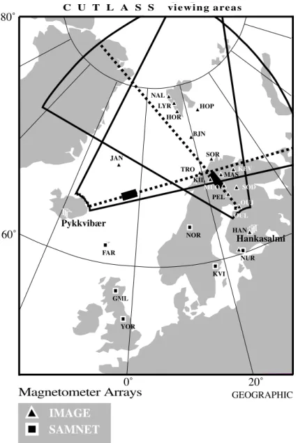
In this study we examined the ionospheric F-region near Tromsø, Norway, using a number of techniques, the main one being the CUTLASS bistatic HF coherent radar. CUTLASS comprises stations at Pykkvibaer in Iceland and Hankasalmi in Finland, and is a component of the international Super-DARN HF radar network (Greenwald et al., 1995). In stan-dard operating mode these radars sweep over a 52◦azimuth sector using 16 evenly spaced beams. This is represented by the fan-shaped regions in Fig. 1. Each beam is gated into up to 75 range bins with spatial resolution of typically 45 km by 100 km at midrange, giving a total field of view of the order of 3×10⁶km2. In standard mode, the integration time for each beam position is 7 s, and the cycle time is 2.0 min.
The operation of HF radars was described by Green-wald et al. (1985). In normal operation these radars detect echoes that are coherently backscattered from∼10-m scale field-aligned ionospheric plasma density irregularities, when the radar beam direction is close to orthogonal to the B field. These irregularities are produced in the high-latitude F-region by plasma drifts and density gradients (e.g. Fejer and Kelley, 1980; Tsunoda, 1988) and drift with the ambient plasma motion (Villain et al., 1985). In each beam the radars measure the line-of-sight Doppler velocity, the backscattered power, and the spectral width of the echo from these struc-tures.
The CUTLASS Iceland East radar looks across the mag-netic meridian and thus is well suited to identifying features moving azimuthally. The Finland radar looks toward the magnetic pole and accordingly is better suited for examining equatorward or poleward moving features. Further details on CUTLASS are available at http://ion.le.ac.uk/cutlass/cutlass. html.
The observations reported here were obtained when CUT-LASS was operating in a non-standard scan mode, optimised for high resolution studies of a specific target region. In this mode three adjacent beams are scanned, with the cen-tral beamed scanned again between each set. The Finland radar thus scanned beams 6, 7, 6, 5, 6, 7, 6, ..., and simi-larly the Iceland East radar scans were centered on beam 14. These beams were sampled each 7 s and the first range gate was set at a distance of 180 km. The radio frequency was in the range 9900–10 000 MHz, appropriate for F-region reflec-tions. These central beams are represented in Fig. 1 by bro-ken lines, and intersect in the F-region just east of Tromsø.
An important feature of radars such as CUTLASS is the measurement of the elevation angle of the backscatter re-turns. This is achieved using an interferometric technique and can assist in discriminating the direction of ground scat-ter and the altitude of irregularity structures (Milan et al., 1997a, b).
We will also present results from a near-vertical incidence ionospheric Doppler sounder experiment that was located near Tromsø. Called DOPE (DOppler Pulsation Experi-ment), this monitored the amplitude and Doppler shift of the ordinary (O-mode) and extraordinary (X-mode) reflections from the F-region at a frequency of 4.45 MHz with a time resolution of 12.8 s. The experiment was described in detail by Wright et al. (1997), where typical results were also pre-sented. Whereas the two CUTLASS radars can measure the horizontal convection velocity components, DOPE provides a measurement of vertical motions in more or less the same part of the F-region.
General information on the ionosphere in this region is available from the Tromsø dynasonde operated by EISCAT. The dynasonde is a digital frequency-agile HF sounder that can operate in a number of modes. During the interval of in-terest here, digital ionograms resolving the O- and X-modes were available from the dynasonde every 3 min. Further de-tails on the EISCAT dynasonde can be found in Sedgemore et al. (1996) and at http://www.eiscat.uit.no/dynasond.html.
Finally, information on the magnitude and structure of D-region absorption can be obtained from the IRIS (Imaging Riometer for Ionospheric Studies) experiment operated at Kilpisj¨arvi (KIL), Finland, by the University of Lancaster. IRIS examines ionospheric absorption of incoming galac-tic radio noise at a frequency of 38.2 MHz with 49 beams and a sampling time of 1 s. Resolution of the riometer is 0.05 dB. The experiment was described in detail by Detrick and Rosenberg (1990) and Browne et al. (1995); further de-tails appear at http://www.dcs.lancs.ac.uk/iono/iris/. Figure 1 shows that KIL is also very near the region where the CUT-LASS beams intersect.
2.2 Ground magnetometer arrays
Magnetometer data were obtained from the IMAGE and SAMNET arrays that span Scandinavia and Svalbard. Sta-tion locaSta-tions are represented by triangles and squares, re-spectively, in Fig. 1. The IMAGE (International Monitor for Auroral Geomagnetic Effects) array was described by L¨uhr (1994) and L¨uhr et al. (1998) and comprises fluxgate magnetometers sampling the geographicX,Y andZ com-ponents of the geomagnetic field each 10 s with a resolu-tion of 0.1–1 nT. Data were rotated into the geomagnetic
res-BJN
OUL
NOR
NUR
KVI
GML
Γ Γ Γ
20˚
0˚
GEOGRAPHIC
60˚
80˚
Hankasalmi
Magnetometer Arrays
YOR
TRO JAN
LYR NAL
HOP
OUJ
IMAGE
SAMNET
HOR
SOR
KEV MAS
SOD
HAN
FAR
PykkvibærΓΓ
Γ
C U T L A S S vi e w i n g a re a s
PEL KIL
MUO
Fig. 1. Map in geographic coordinates showing CUTLASS beams and ranges of interest, and IMAGE and SAM-NET magnetometer locations. Shaded boxes depict ionospheric reflection re-gions for ground scatter recorded by beam 6 of the Finland radar and beam 14 of the Iceland East radar. The DOPE Doppler sounder was located just east of Tromsø, and the IRIS imaging ri-ometer at KIL.
olution of 0.25 nT. Further details appear in Yeoman et al. (1990a) and at http://samsun.york.ac.uk/samnet home.html. 2.3 Solar wind and DMSP data
Solar wind data presented in this paper are from the WIND spacecraft, which at the time of interest was located up-stream near GSE(x, y, z) = (172.5, −5.6, 11.23)RE. We used solar wind and magnetic field data from the SWE (So-lar Wind Experiment) and MFI (Magnetic Fields Investiga-tion) instruments, respectively. Further information on these experiments is given in Ogilvie et al. (1995) and Lepping et al. (1995), and at http://www-istp.gsfc.nasa.gov/istp/wind/ wind.html.
General information on magnetospheric topology was ob-tained by reference to ion and electron flux data from the DMSP F12 spacecraft. This is one of a series of space-craft in an approximately 830 km altitude Sun-synchronous,
101-min period polar orbit. Spectra of low energy ion and electron fluxes at high-latitudes are produced by the SSJ/4 electrostatic analyzer instruments, described by Hardy et al. (1985). Further details on DMSP may be obtained from http://sd-www.jhuapl.edu/Aurora/. The use of DMSP par-ticle spectra to infer the locations of the magnetospheric boundaries has been discussed by Newell and Meng (1988, 1992) and Newell et al. (1989, 1991).
3 Observations
3.1 Solar wind
Fig. 2. (a, left)WIND solar wind plasma and magnetic field data, 07:00–13:00 UT, 23 February 1996. Top three panels show the solar wind speed, then ion density, dynamic pressure, and magnetic field, all in GSM coordinates. For the bottom panel the thin solid line represents theBx component, the dotted line theBycomponent, and the thick solid line theBzcomponent. Vertical dotted lines denote times when
Bzturns negative (labelled “A”), when solar wind pressure begins to drop (“B”) and reaches minimum (“C”), and the interval of oscillations considered in detail (“D” to “E”).
(b, right)Power spectrum of three components of the IMF and solar wind dynamic pressure, 09:33–11:33 UT (spacecraft time; 10:20– 12:20 UT on the ground), 23 February 1996. Resolution is approximately 0.14 mHz and time series are unfiltered. Vertical dotted line indicates frequency of 1.6 mHz seen in ionospheric and ground magnetometer data.
was in the range 2+ to 3+, but had been low over the previous few days (6Kp= 8.7, 14 and 18 on 21, 22 and 23 February, respectively).
WIND observations of the solar wind plasma and mag-netic field conditions from 07:00 UT to 13:00 UT on 23 February are presented in Fig. 2a. The top panel shows solar wind velocity, with density and pressure in the next panels. The bottom panel presents the corresponding WIND IMF data in GSM coordinates, where the thick solid line rep-resents theBzcomponent, the dotted line represents theBy
component, and the thin solid line represents theBx compo-nent.
The solar wind speed was generally in the rangeV =405– 430 km s−1 throughout the interval shown. This includes a
sharp increase from∼410 to∼430 km s−1around 08:50 UT
and a subsequent decrease at∼09:22 UT.
theBxandBzcomponents are strongly negative. This is fol-lowed by a sharp decrease in ion density, fromn∼20 cm−3at 08:41 UT (“B”) to 6 cm−3at 08:57 UT (“C”). This caused a decrease in solar wind pressure,nV2, by a factor of about 3 between these times. The pressure decrease commenc-ing at 08:41 UT (“B”) also initiates a strong positive tran-sition ofBy, which later goes briefly negative again between 09:59 UT and 10:12 UT.
We have calculated the propagation lag from WIND to the magnetopause and ionosphere using the formula given by Lockwood et al. (1989) and assuming an Alfv´en wave transit time through the magnetosphere to the ionosphere of 2 min. The time lag from WIND to the ionosphere varies from nearly 50 min at “A” and “B” to 47 min for the later events. For simplicity, we henceforth assume a fixed 47-min lag from the satellite to the ionosphere. This will not affect the discussion of the sequence of observations.
Accordingly, the negative pressure pulse at 08:41 UT (“B” in Fig. 2a) should reach the ionosphere at ∼09:28 UT, and the maximum depth of the pressure pulse (“C”) occurs at the ionosphere at 09:44 UT. The solar wind pressure commences recovery to near its original value at∼09:20 UT (at WIND). Periodic solar wind pressure fluctuations with amplitude up to 25% of the total amplitude occurred for some hours after the pressure decrease. These commenced around 09:33 UT at WIND and 10:20 UT at the ionosphere (“D”), and ended at WIND around 11:33 UT (“E”) and 12:20 UT at the ionosphere. Figure 2b shows power spectra of the three components of the IMF and the solar wind dynamic pres-sure meapres-sured by WIND between 09:33 UT and 11:33 UT (∼10:20–12:20 UT at the ionosphere). The spectra were computed using a single FFT, weighted by a Hanning win-dow and with no detrending or filtering. Frequency resolu-tion of the spectra is approximately 0.14 mHz. The spec-tra show a peak in solar wind pressure variations with a fre-quency near 1.5–1.7 mHz (period 10–11 min), which is dou-ble the power of the adjacent peaks. The IMFBycomponent shows peaks near 1.6 and 2.1 mHz, theBz component has a peak near 2.1 mHz only, and no clear peak is present in the
Bx spectrum. Note that there do not appear to be any step-like transients in the solar wind pressure or in the Bx and
Bzcomponents during this interval (see Fig. 2a). However, there is a significant transient variation inBy, as mentioned earlier.
According to a formula given by Farrugia et al. (1989), the negative solar wind pressure pulse would have resulted in sunward motion of the magnetopause of∼1.9RE, and the subsequent fluctuations would have caused motions of the order of 0.2–0.4RE.
3.2 Cutlass radar
HF radar data are typically presented in the form of whole-day range-time parameter plots for a particular beam. Pa-rameters of interest are the power, the line-of-sight velocity, the elevation angle, and the spectral width (in m s−1) of the
returned signal. Backscatter regions of small velocity and
spectral width are normally considered to indicate ground scatter and their plotting is usually suppressed. In the fol-lowing plots we have not suppressed this low velocity, low spectral width information.
Figure 3 presents combined range-time-velocity plots for beam 6 from the Finland radar and beam 14 from the Ice-land East radar, from 09:00 to 13:00 UT on 23 February. Panels (a) and (c) present Doppler velocity data that has been identified as coming from ionospheric scatter, while panels (b) and (d) present Doppler velocity data that has been identified as coming from ground scatter. Milan et al. (1997a) have discussed the distinction between ionospheric and ground scatter in HF radar returns. Figure 3 shows many complicated features. Milan et al. (1998) presented plots of the Finland beam 5 power, velocity and elevation angle for this day, and provided a detailed discussion of the features observed.
We consider first the Finland velocity plot shown in Fig. 3a. There is a prominent zone of periodic high veloc-ity poleward moving features (negative velocveloc-ity = away from radar = red), commencing near 09:20 UT between 76–80◦ magnetic latitude (range gates 45–50) and moving to 72– 76◦latitude (gates 40–45) by 13:00 UT. The corresponding power level plot (not presented here but see Milan et al., 1998) shows that this zone is associated with high backscat-tered power. In radar data the cusp footprint is associated with a complex Doppler spectrum and broad spectral width (Baker et al., 1995). The spectral width plot (not given) shows irregular and high spectral widths (450 m s−1) from
76–80◦latitude at 09:30 UT. Finland beam 6 points 18◦west of geographic north and the high velocity, high spectral width zone lies magnetically poleward and somewhat west of Sval-bard. We interpret this zone as the signature of the dayside auroral oval, and henceforth refer to radar returns from this region as ionospheric scatter. The negative, pulsed veloc-ity structures throughout the interval represent antisunward flow, and are characterised by broad radar spectral widths. As such, they are typical of the radar cusp scatter under IMF
Bz south conditions (Pinnock et al., 1993, 1995; Provan et al., 1998; Neudegg et al., 1999).
The DMSP F13 spacecraft passed over the arctic region northwest of Svalbard around 08:47 UT on this day. The ob-served particle energies and fluxes indicate that the cusp and open/closed field line boundary were located∼75◦magnetic latitude. This lends confidence to our identification of the high velocity region as cusp/dayside auroral oval and agrees with the magnetometer observations presented later.
The solar wind pressure decrease arriving at the iono-sphere around 09:30 UT appeared to initiate or enhance pe-riodic antisunward flow bursts in the cusp ionosphere that lasted about two hours. The period of the features here is of the order of 10 min. The equatorward movement of the low-latitude boundary of this flow zone at∼10:45 UT is in-dicative of an expanding polar cap resulting from dayside reconnection under IMFBzsouth conditions.
SUPERDARN PARAMETER PLOT
Finland and Iceland East: vel
23 Feb 1996
70 75 80
Magnetic Latitude 70 75 80
Magnetic Latitude -800
-600 -400 -200 0 200 400 600 800
Velocity (ms
-1
)
Ionospheric scat only
70 75 80
Magnetic Latitude 70
75 80
Magnetic Latitude -24
-18 -12 -6 0 6 12 18 24
Velocity (ms
-1
)
Ground scat only
100 110 120 130
Magnetic Longitude 100
110 120 130
Magnetic Longitude -800
-600 -400 -200 0 200 400 600 800
Velocity (ms
-1
)
Ionospheric scat only
09 09 10 10 11 11 12 12 13
UT 90
100 110 120 130
Magnetic Longitude
09:00 09:30 10:00 10:30 11:00 11:30 12:00 12:30 13:00 UT
90 100 110 120 130
Magnetic Longitude -24
-18 -12 -6 0 6 12 18 24
Velocity (ms
-1
)
Ground scat only
A B C D E
Iceland beam 14, ground scatter Iceland beam 14, ionospheric scatter Finland beam 6, ground scatter Finland beam 6, ionospheric scatter (a)
(b)
(c)
(d)
Fig. 3. Range-time-velocity plot for Finland beam 6 ionospheric scatter (top panel,(a)and ground scatter(b), and Iceland East beam 14 ionospheric scatter(c)and ground scatter(d), over 09:00–13:00 UT on 23 February 1996. Vertical dotted lines indicate approximate arrival times at the ionosphere of events labelled “A” to “E” in Fig. 2. Finland ground scatter in (b) before 10:24 UT, indicated by the vertical dashed line, is from behind the radar.
in magnetic latitude (range ∼1000–1500 km). Figure 1 of Milan et al. (1998) shows that this region is characterised by high backscattered power (40 dB) and high elevation an-gles. Spectral widths are low (<100 m s−1). We denote this
as ground scatter. Milan et al. (1998) have provided a de-tailed discussion on the interpretation of the elevation angle
data and the location of ground scatter regions in front of and behind the radar on this day.
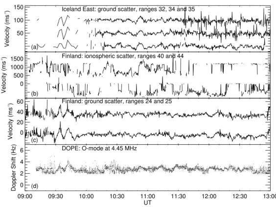
so-0 500 1000 1500
Velocity (ms
-1)
(b)
Finland: ionospheric scatter, ranges 40 and 44
0 20 40 60
Velocity (ms
-1 )
(c)
Finland: ground scatter, ranges 24 and 25
09:00 09:30 10:00 10:30 11:00 11:30 12:00 12:30 13:00
UT 0
2 4 6
Doppler Shift (Hz) (d)
DOPE: O-mode at 4.45 MHz 50
100 150
Velocity (ms
-1 )
(a)
Iceland East: ground scatter, ranges 32, 34 and 35
SUPERDARN PARAMETER PLOT
CUTLASS Finland and Iceland East (vel) and DOPE
23 Feb 1996
(54)normal (cw) scan mode (127)
Fig. 4.Stacked velocity-time plot of CUTLASS and DOPE Doppler oscillations, 09:00–13:00 UT, 23 February 1996. The same CUTLASS beams are shown as in Fig. 3. The panels show, from top to bottom, Iceland East ground scatter, Finland ionospheric scatter, Finland ground scatter, and HF Doppler O-mode.
lar wind pressure decrease labelled “B” in Figs. 2a and 3. Alternating features due to velocity oscillations of amplitude ±20 m s−1or less, with period of
∼10 min, are present for at least 3 h, and have a very similar shape over 4–8 range gates, i.e. over 180–360 km in latitude. We emphasise that these are ground backscatter features, not returns from field-aligned ir-regularity structures in the usual sense.
Now consider the Iceland East range-time-velocity plots, shown in Figs. 3c and d. The transition at 10:00 UT cor-responds to the radar switching into the special high reso-lution mode. Of interest is the zone of low velocity bands in the bottom panel (d), commencing around 09:30 UT and visible during the entire plot interval. The bands extend over about 10 range gates (∼450 km) and are associated with high power levels, very low spectral widths, high elevation angles (25–30◦), and line-of-sight velocities of the order of ±10– 20 m s−1. Detailed plots appear in Menk et al. (2001). The
bands are due to velocity oscillations that were essentially si-multaneous across the field of view and exhibited a 10-min periodicity. The zone of velocity structures gradually moved westward, toward the radar. As for the Finland radar, we interpret this entire zone of velocity oscillations as ground scatter.
The most likely explanation of the low velocity bands seen
by both radars is that the ground scatter signal is experienc-ing a Doppler shift durexperienc-ing each traversal through the iono-sphere, for example, in response to motion of the ionospheric plasma. The Doppler shifts are periodic and commence at the same time as the negative solar wind pressure pulse would reach the ionosphere. To investigate this further, we next consider results from the vertical incidence Doppler sounder experiment, DOPE.
3.3 HF Doppler sounder and digisonde
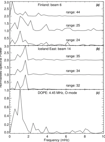
0.5 1.0 1.5 2.0 2.5 3.0
(a)
Finland: beam 6
range: 44
range: 25
range: 24
0.5 1.0 1.5 2.0 2.5 3.0
Normalised Spectral Power
(b)
Iceland East: beam 14
range: 35
range: 34
range: 32
0 2 4 6 8 10
Frequency (mHz) 0.0
0.2 0.4 0.6 0.8 1.0
(c)
DOPE: 4.45 MHz, O-mode
Fig. 5. Stacked power spectra (0.3 mHz resolution), over 10:20– 11:20 UT, for(a)Finland beam 6 radar velocities(b)Iceland beam 14 radar velocities, and(c)DOPE vertical incidence Doppler shifts.
Ionograms from the Tromsø dynasonde show that for ver-tical incidence, the 4.45 MHz O-mode group height was ∼260–265 km over this interval, withfoF2∼5.4 MHz. The ionosphere did not appear to be particularly disturbed before 13:00 UT, and the DOPE oscillations were observed from just below the peak of the F2-region.
Power spectra of the Finland, Iceland East and DOPE Doppler oscillations over the interval 10:20–11:20 UT (i.e. from the end of pressure pulse – labelled “D” in Figs. 2b and 3, and covering the first half of the pressure oscillations) are compared in Fig. 5, for most of the range bins presented in Fig. 4. The DOPE data were low pass filtered at 11 mHz and the spectra were computed with a single FFT then nor-malized to facilitate comparison. Resolution of all the spec-tra is about 0.3 mHz. The Iceland East ground scatter specspec-tra (Fig. 5b) show a clear peak∼1.7 mHz at ranges correspond-ing to the low velocity backscatter pulsations. The Finland plots (panel a) is more complicated, with extra spectral fea-tures present. This is not surprising for the auroral oval iono-spheric scatter (range gate 44). Finland beam 6, ranges 24 and 25 and DOPE (panel (c)) are essentially looking at the same part of the ionosphere and show prominent spectral peaks near 1.1 mHz. Finland beam 6, range gate 24 also shows a secondary peak at 1.7 mHz. Note also the small peaks around 6–8 mHz present in the Finland ground
scat-Fig. 6a. MagnetometerH-component data from the IMAGE and SAMNET arrays, 23 February 1996. Time series records for 09:00– 13:00 UT. Vertical dotted lines indicate approximate arrival times at the ionosphere of events labelled “A” to “E” in Figs. 2 and 3.
ter and DOPE spectra.
3.4 Ground magnetometer data
Figure 6a presents stacked H-component time series plots from representative IMAGE and SAMNET magnetometer stations for 09:00–13:00 UT (covering the IMF Bz south-ward turning, the solar wind pressure pulse, and the arrival of oscillations at the ionosphere), band-pass filtered between 1 and 10 mHz. Vertical dotted lines, labelled “A” to “E”, indicate arrival times at the ionosphere of the features iden-tified in Figs. 2a and 3. Figure 6b is a higher resolution plot showing the H- and D-components (solid and dotted lines, respectively) over 09:10–10:10 UT (covering the IMF
Bz southward turning and the solar wind pressure pulse ar-rival at the ionosphere) for the same stations.
All stations recorded a large bipolar event starting around 09:30 UT, coincident with the presumed arrival at the iono-sphere of the solar wind pressure pulse (recall that because we assumed a uniform propagation time, the solar wind pres-sure decrease labelled “B” actually reaches the ionosphere around 09:30 UT). This was followed for some hours by Pc5 pulsation activity that was remarkably similar at all stations
Fig. 6b. Expanded time series records for 09:10–10:30 UT, where
H-component is the solid line andD-component is the dotted line. Vertical dashed lines indicate events identified earlier.
peak, and the phase seems to change, between SOR (67.2◦) and BJN (71.3◦) latitude. The magnetometer time series also show two transient, pulse-like events starting around 09:20 UT at∼74◦magnetic latitude (HOR), coincident with the southward turning ofBz reaching the ionosphere. The pulses are clearest in theH-component and appear somewhat later at other latitudes. At this time shorter period (frequency 6–8 mHz) pulsations commenced at lower latitudes. These were most prominent∼66–67◦latitude.
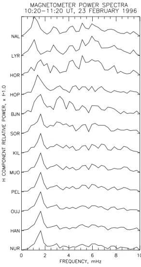
Stacked power spectra for the same magnetometer H -components are presented in Fig. 6c. This is the same time interval shown in Fig. 5, although similar features were present for some hours in the magnetometer spectra. The spectra in Fig. 6c were weighted byf1.0, to better display higher frequency features, and normalized to facilitate com-parison. Spectral resolution is∼0.3 mHz. The spectra show a clear peak around 1.6–1.7 mHz at all stations<75◦latitude. Smaller peaks∼6–8 mHz are also present at many stations.
Signals at the highest latitude stations (HOR, LYR and NAL, 74–76◦magnetic latitude) have more high frequency activity and are somewhat different in appearance to the lower latitude signals. This suggests they are probably as-sociated with the dayside auroral oval and open/closed field line boundary, in agreement with the CUTLASS and DMSP observations discussed earlier.
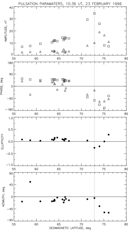
We now consider the 1.6–1.7 mHz magnetic pulsations in more detail. The variation in amplitude, phase, ellipticity and azimuth with geomagnetic latitude for this frequency is
Fig. 6c.Power spectra for 10:20–11:20 UT (resolution is 0.3 mHz). Spectra were weighted byf1.0and normalized.
shown in Fig. 7. These measurements were obtained using complex demodulation (Beamish et al., 1979; Chisham and Mann, 1999) over a bandwidth of 1.5–2.3 mHz, yielding a demodulate value each 12 min. The points plotted in Fig. 7 are for the time interval centred on 10:36 UT, but other times give similar results. The plots show a peak in amplitude, a re-versal in phase, and linear generally north-south polarization, all consistent with a field line resonance (FLR) around 72– 73◦geomagnetic latitude. The dotted vertical line near 73◦ indicates the latitude of the amplitude peak. The full width at half power (FWHP) of the amplitude-latitude profile indi-cates a resonance scale size at the ground of the order of 4◦ in latitude, i.e.∼400 km.
Fig. 7. Variation in amplitude (top panel), phase, ellipticity and azimuth angle (bottom) for 1.6 mHz geo-magnetic pulsations at 10:36 UT on 23 February 1996. In the upper two panels squares denote H-component values and trianglesD-component.
Using IMAGE data, Mathie et al. (1999b) showed that dis-crete FLRs occur at the eigenfrequency of the continuum determined from the cross-phase between pairs of adjacent magnetometer stations (Waters et al., 1995). We measured the field line eigenfrequency in this way (Menk et al., 2001) and during the morning of 23 February, it varied smoothly from 1.6±0.3 mHz at 71.4◦latitude, to 8.0±0.3 mHz at 66◦, and 15±1 mHz at 62◦. Complex demodulation plots in the same format as Fig. 7 but for a frequency of 8.0 mHz show a small peak in power, a reversal in phase and changes in ellip-ticity and azimuth characteristic of a FLR, near 66◦latitude. Cross-phase measurements can be used to estimate the
width,Qand damping of the resonance (Menk et al., 1999). For the 1.6–1.7 mHz signal the resonance width in the iono-sphere is thus estimated at 90–150 km, theQis 1.5 to>3, and the damping factor∼0.3. We could not obtain a cross-phase resonance signature at≥75◦latitude. This is indica-tive of open field lines at these latitudes (Ables et al., 1998). 3.5 Imaging riometer observations
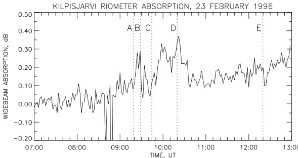
Fig. 8.Cosmic noise absorption over 07:00–13:00 UT for the wideband KIL riometer. Resolution is 0.05 dB. Vertical dotted lines indicate approximate arrival times at the ionosphere of events labelled “A” to “E” in Figs. 2 and 3.
to 90 km altitude of cosmic noise absorption over a square 240×240 km area, measured each 15 or 120 s. The IRIS facility also includes a widebeam riometer, with a −3 dB beamwidth of∼94◦. Figure 8 shows the variation in received power over 07:00–13:00 UT, measured with the widebeam riometer. For brevity other beams and absorption maps are not shown here, but they indicate the same general features. The dotted vertical lines in the figure denote the arrival times at the ionosphere of the events discussed earlier, including the southwardBz turning at 09:19 UT (“A”) and the initial solar wind pressure decrease near 09:28 UT (“B”). A sud-den increase in absorption (i.e. decrease in received signal power), commencing at 09:19 UT, was followed at 09:28 UT by a decrease in absorption, lasting∼20 min. Enhanced ab-sorption between∼09:50–10:35 UT coincides with the solar wind pressure minimum in Fig. 2a.
4 Discussion
4.1 Effects of solar wind variations
In this paper we are principally concerned with the responses of the ionospheric sounders and magnetometers to the sudden decrease in solar wind pressure arriving at 09:30 UT. This was preceded by a southward turning ofBzat 09:19 UT, al-thoughBz had been negative for about 45 min just before then and IMF conditions conducive to dayside reconnection occurred throughout the interval under consideration.
Inspection of Fig. 3 and high resolution velocity-time plots not given here show that two narrow poleward moving flow bursts were recorded by the Finland radar between 09:20– 09:30 UT. These started near 76◦latitude and extended to 79◦ latitude at a rate of∼1.5–2 km s−1, while the flow velocity
within the flow channels was∼1.0 km s−1. The high
reso-lution magnetometer time series in Fig. 6b shows that near the same time, a pair of pulses was observed at HOR (74.0◦ geomagnetic latitude), appearing somewhat later at other lat-itudes. Taking into account the longitudinal spread of the sta-tions (HOR is westward of HOP), the data suggest the pulses were travelling mostly eastward at 1.5–3 km s−1. This was
followed at lower latitudes by 6–8 mHz pulsations. A sud-den increase in cosmic noise absorption was recorded by the riometer at 65.8◦latitude between 09:20–09:30 UT.
These observations are consistent with the ionospheric sig-natures of reconnection at the magnetopause (e.g. Pinnock et al., 1993; Øieroset et al., 1997). In particular, south-ward Bz turnings are connected with flux transfer events (FTEs). SuperDARN radar observations of the cusp have shown that the ionospheric footprint of FTEs is characterised by pulsed poleward moving flow bursts, known as pulsed ionospheric flows (PIFs) or flow channel events (FCEs), near the polar cap boundary (Pinnock et al., 1995; Provan et al., 1998; Provan and Yeoman, 1999; Neudegg et al., 1999; McWilliams et al., 2000). The relationship between PIFs, FCEs and FTEs is discussed more thoroughly in Wild et al. (2001). A detailed discussion of the mapping of FTEs to the ionosphere in PIFs appears in McWilliams et al. (2001).
The poleward flow bursts in the Finland velocity plot are similar in appearance to reported PIFs and commenced when
Hemi-B
1000
0
Range (km)
ray
A
ray
B
2000
v
iv
dB
1000
0
Range (km)
ray
C
2000
v
iv
d(b)
10:24-13:00 UT
(a)
09:00-10:24 UT
-1000
-1000
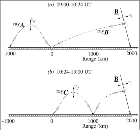
Fig. 9.Likely ray paths for the Finland radar. (a)09:00–10:24 UT. Ray A rep-resents ground scatter reflected from the F-region behind the radar, and experi-encing ionospheric Doppler oscillations
vd. Ray B represents ionospheric scat-ter from the cusp F-region, with line-of-sight Doppler velocityvi.
(b)10:24–13:00 UT. Ray C represents simultaneous F-region reflected ground scatter and 1.5 hop mode ionospheric scatter from the auroral F-region.
sphere (Southwood, 1987; Chaston et al., 1993; Provan et al., 1998).
The sudden decrease in solar wind pressure commencing at 09:30 UT then appeared to enhance the flow bursts, trig-gered F-region Doppler oscillations, initiated 1.6–1.7 mHz magnetic pulsations with a large bipolar event, and caused a reduction in riometer absorption. The flow bursts, Doppler shifts and magnetic pulsations occurred over a wide region, lasted for some hours, and exhibited the same period as so-lar wind pressure fluctuations. The IMFBzcomponent was southward throughout the pressure decrease, and shows some fluctuations but at a higher frequency than observed on the ground (Fig. 2b). Thus, while conditions were favourable for reconnection, and the radar cusp region flow channels appear to be reconnection related, it is the changes in solar wind pressure that seem to be driving the ionospheric and magnetic perturbations.
4.2 Properties of the ionospheric oscillations
Here we discuss the spatial variation in phase and the loca-tion, scale size and direction of motion of the ionospheric oscillations. We first consider phase motion of the oscilla-tory features in the Finland Doppler velocity record. For this purpose we determined the phase delays at several times after 10:30 UT, using stacked velocity-time plots and phase spec-tra (not shown here) for several range gates in beam 6.
For the ground scatter velocity oscillations the phase delays suggest the oscillations (which are being observed
mostly equatorward of the FLR) are moving poleward at 1– 5 km s−1. This sense of motion is consistent with the change
in phase of magnetic pulsations associated with resonance (Walker et al., 1979). Milan et al. (1997a) pointed out that the CUTLASS radars can observe ground scatter from both in front of the radar and from behind the radar, in a rear lobe of the antenna pattern. Accordingly, Milan et al. (1998) argued, from an analysis of radar elevation angles, that ground scatter observed at Finland before 10:24 UT on this day is from be-hind the Finland radar. This time is identified by the dashed line on Fig. 3b. Returns are obtained from behind the radar due to the low F-region electron density in the high-latitude winter ionosphere compared to lower latitudes. However, between 10:24 UT and 14:00 UT, the high-latitude F-region electron density increased sufficiently so that ground scat-ter from in front of the radar is of higher backscatscat-ter power and hence dominates. A similar analysis of elevation angles demonstrates that the ground scatter from Iceland (Fig. 3d) is from in front of the radar.
Motion of the ionospheric backscatter flow bursts (associ-ated with the auroral oval) over the times of interest are also generally poleward, at 2–3 km s−1. Prikryl et al. (1998)
wind-magnetosheath magnetic and electric fields at the dayside magnetopause, while FLRs were excited on magnetic shells adjacent to the noon magnetopause.
For the Iceland East radar the Doppler velocity ground scatter oscillations (Fig. 3d) appear to move westward be-fore about 11:00 UT, and eastward, or have no net east-west motion afterward. The speed is variable, corresponding to an azimuthal wave number of the order of −2 to −5 be-fore 11:00 UT. This agrees well with the magnetometer mea-surements. Inspection of Fig. 4 and higher resolution plots not given here shows that the ionospheric oscillations are in phase, or nearly in phase, in the Finland, Iceland East and DOPE echoes.
Now we consider the location where the radar oscillations are observed. Figure 9a shows the likely ray-path geometry for the CUTLASS Finland beam between about 09:00 UT and 10:24 UT (including the southward turning – “A” in Fig. 2a – and the solar wind pressure pulse reaching the iono-sphere). Information on identifying the ray paths comes from the different properties of ionospheric and ground scatter, as described earlier, and from interferometer measurements of elevation angle (Milan et al., 1997a, b, 1998). Following the earlier discussion on the location of the ground scatter, ray A represents the ground scatter return reflected from the F-region behind the radar, and ray B represents the F-F-region ionospheric scatter. Motions in the cusp ionosphere are indi-cated by the orthogonal velocitiesvi. Since the calculation of range is based on time of flight, the ionospheric Doppler os-cillationsvdin ray A will occur at approximately half the dis-tance indicated on the range-time plots. The same will apply to the Iceland East ground scatter observations. These iono-spheric target regions are represented by the shaded boxes in Fig. 1, and span 64–68◦N geographic for the Finland radar, and 16 to 1◦geographic longitude for Iceland East.
After∼10:24 UT high elevation angles in the Finland re-turns for larger ranges (see Milan et al., 1998) suggest the ray path shown in Fig. 9b. This mode, ray C, provides simul-taneous F-region reflected ground scatter and 1.5 hop iono-spheric scatter from the auroral F-region. High velocity Pc5 features have been reported previously in HF radar data at slightly lower latitudes (Yeoman et al., 1990b, 1997) and in the cusp (Matthews et al., 1996), although not in the context of 1.5 hop returns as discussed here.
The ground scatter Doppler shift regions for the two radars are separated by several hundred km and indicate that the ionospheric oscillations span at least 25◦ in longitude. In addition, the observation of ground scatter from behind the Finland radar before 10:24 UT indicates that the oscilla-tions extend over at least 16◦ in latitude. The magne-tometer observations also showed that the pulsations ex-tend over at least 20◦ (2200 km) in latitude. The magne-tometer observations in Fig. 7 and the cross-phase analysis show that the 1.6–1.7 mHz resonance region is around 72– 73◦magnetic latitude (HOP, HOR, BJN). The 1.6–1.7 mHz ionospheric Doppler oscillations were observed 6–7◦(660– 770 km) equatorward of this region. Wright et al. (1998) had previously reported the appearance of Pc5 pulsations in the
ionosphere, up to 8◦equatorward of a broad FLR identified using the IMAGE magnetometer array.
Finally, we consider the ionospheric velocity vectors for the ground scatter,vd for ray A before 10:24 UT and ray C after 10:24 UT. We assume that (a) the Finland and Iceland East radars and DOPE are examining the same altitude in the ionosphere, and (b) the radar and DOPE Doppler shifts are due solely to vertical motions of the reflection point. Further-more, note that rays A and C in Fig. 9 traverse the Doppler shift region twice, so the resultant velocity should be halved. Under these assumptions, the largest amplitude Doppler velocity oscillations observed by the CUTLASS radars each correspond to peak velocity components of about±10 m s−1,
and the DOPE Doppler oscillations to±30 m s−1vertically,
with equivalent motions of the reflection point of a few km. Although assumption (b) ignores the effects of redistribution of plasma or changing magnetic field, it is instructive to es-timate the Doppler shifts that would result from particle mo-tions driven by downgoing transverse Alfv´en waves. If the velocity and magnetic field perturbations are linearly related, then (Rishbeth and Garriott, 1964)
1V ≈ √1B
µ0ρ
r ω
vin
, (1)
whereρ is the mass density of the F2-region plasma (com-prising mostly O+ions at a concentration of∼3×10¹¹m−3), ωis the angular frequency of the pulsation, andvinis the ion-neutral collision frequency in the F-region,∼1 s−1. Hence,
for 1B∼10 nT (assuming no attenuation between the be-tween the ionosphere and the ground) andω∼0.01 rad s−1,
we haveV ∼10 m s−1, comparable to the magnitude of the
observed Doppler oscillations.
These observations highlight the ability of ground scat-ter measurements to extend the scope and capability of HF radars for monitoring perturbation features in the ionosphere. We note in this regard that auroral backscatter radars (such as STARE) are limited by the threshold for the formation of ir-regularities, which is of the order of 15–20 mV m−1(Cahill
et al., 1978). Importantly, downgoing fast (compressional) mode waves are characterised by small ionospheric electric fields (Kivelson and Southwood, 1988; Yeoman and Lester, 1990), and are, therefore, more readily detected using ground scatter measurements.
Poole et al. (1988) showed that three separate mechanisms contribute to pulsation-driven ionospheric Doppler oscilla-tions, while Sutcliffe and Poole (1989) gave a detailed dis-cussion of the validity of theE ×B mechanism (their V2
to downgoing fast mode waves are smaller than for shear Alfv´en mode waves. Therefore, it is difficult to anticipate the ionospheric velocities we would expect to see here, but the inferred velocity components probably represent an up-per bound on the real case.
4.3 Pulsation source mechanism
The magnetometer and radar observations show 1.6–1.7 mHz pulsations with similar appearance over at least 20◦ in lati-tude and 25◦in longitude. These were triggered initially by the solar wind pressure pulse, and continued for some hours. The solar wind dynamic pressure was variable during that time, with a spectral peak∼1.6 mHz (Fig. 2b). The IMF was also variable, with spectral peaks around 1.6 mHz inBy and 2.1 mHz in all three components. Since transient fluctuations are often present in the solar wind pressure and IMF, caution is needed when interpreting such spectra. However, signif-icant transients do not seem to be present during the inter-val considered, except inBy. The extended interval of 1.6– 1.7 mHz ionospheric and magnetic oscillations is, therefore, most likely due to (a) periodic solar wind pressure variations, (b) periodicity in the reconnection rate, or (c) some combi-nation of these mechanisms. The most likely explacombi-nation of the spatial extent of the observations is that one or both of these mechanisms launched fast mode waves into the mag-netosphere, driving resonances where the field line eigenfre-quency and incoming wave freeigenfre-quency match, and forced field line oscillations elsewhere (Hasegawa et al., 1983). Complex demodulation (Fig. 7) and cross-phase analysis demonstrates that the pulsations coupled to FLRs around 72–73◦ geomag-netic latitude, equatorward of the predominantly reconnec-tion driven flows at 74–80◦.
Solar wind impulse-driven pulsations can have similar sig-natures to localized field line reconnection events (Farrugia et al., 1989; Sibeck, 1990). In our data, a reasonably local-ized pulse occurred at 09:19 UT (the southwardBzevent) at latitudes near 74◦, where the Finland radar observed recon-nection related flows. This propagated relatively slowly to other latitudes. In contrast, the pressure decrease at 09:30 UT produced a bipolar response at more widely spaced locations than the reconnection events, and was followed by sustained Pc5 signals driven at the same frequency as the solar wind pressure oscillations.
Yeoman et al. (1997) presented high resolution mea-surements of 7–8 mHz magnetic pulsations recorded with IMAGE magnetometers, and simultaneous CUTLASS Fin-land backscatter velocity oscillations of magnitude 100– 300 m s−1. The pulsations were most probably due to an
impulse-driven cavity/waveguide resonance, which coupled to FLRs whose width in the ionosphere over Tromsø was of the order of 60 km. Such a small scale-size means that the FLR is highly attenuated in the ground magnetometer data. Our signals have considerably larger scale size, al-though the cross-phase measurements, which are based on the difference between signals at adjacent stations, yielded a smaller scale size (70–90 km) than the FWHM
measure-ments (∼400 km). This may reflect the effects of spatial integration on the magnetometer signal (Poulter and Allan, 1985). The estimated damping factor of 0.3 points to the ex-istence of damping mechanisms other than Joule dissipation (Yeoman et al., 1997).
Solar wind pressure pulses of the magnitude observed here are believed to be fairly common (Sibeck, 1990). Ground-based observations associate them with ringing type mag-netic pulsations with periods of a few minutes (Takahashi et al., 1988; Farrugia et al., 1989; Sibeck, 1990), including field line resonances (Potemra et al., 1989; Warnecke et al., 1990; Parkhomov et al., 1998; Prikryl et al., 1998).
Examining a large magnetospheric compression event, Takahashi et al. (1988) found
(i) 1.1–1.7 mHz compressional waves which could have been due to a global fast-mode cavity resonance, (ii) standing 3–6 mHz Alfv´en waves (i.e. FLRs), and (iii) 3–8 mHz irregular disturbances near the magnetopause. The magnetopause and bow shock also seemed to execute 1.1–1.7 mHz motions. Potemra et al. (1989) also found that quasi-periodic variations in the solar wind density may drive transient magnetospheric ULF waves at the same frequency. These may excite local FLRs. Takahashi et al. (1988) be-lieved the frequency of the 1.1–1.7 mHz compressional wave was too low to couple to standing Alfv´en waves. How-ever, Mathie et al. (1999 a, b) demonstrated the existence of 1.7 mHz field line resonances at high-latitudes, and discussed their origin in terms of magnetospheric waveguide modes.
Farrugia et al. (1989) have shown that magnetic oscilla-tions may be observed over a wide range of latitudes and longitudes with the same frequency as magnetopause mo-tions. The meridional motion of the signals across the ground corresponds to tailward propagation in the magnetosphere, at∼11 km s−1. Sibeck (1990) presented a detailed
descrip-tion of this process. Significantly, large amplitude solar wind dynamic pressure impulses, recurring on time scales of 5– 15 min, are a fairly common feature just upstream of the bow shock. The ground signatures of these pressure pulses in-clude bipolar north-south flows and magnetic perturbations at high-latitude stations. This is very similar to what we have seen for the event studied here. For example, a prominent feature of Fig. 3 is the two velocity features in the Finland radar, associated with north-south flows in the cusp and F-region Doppler oscillations at lower latitudes, triggered by the solar wind pressure pulses at 09:30 UT. Similarly, the presence of bipolar magnetometer pulses evident in Fig. 6b agrees with the response to sudden expansions predicted by Araki and Nagano (1988).
was followed by a decrease in absorption while the solar wind pressure was decreasing. This is also reasonable, since the resultant sudden magnetospheric expansion (rather than a compression, as discussed by Sibeck) would distribute the population of energetic electrons over a larger volume, thereby decreasing the flux at the ground. The reason for the observed enhancement in absorption while the solar wind pressure was at its minimum is not clear.
Parkhomov et al. (1998) examined geomagnetic pulsations associated with a negative solar wind pressure pulse (by a factor of∼3) and found this initiated 2.3 mHz oscillations across a wide range of latitudes, lasting for about 25 min. These appeared to couple to a 3 mHz FLR, which they argued was the minimum resonance frequency available to incom-ing 2.3 mHz fast mode waves. They interpreted the 2.3 mHz pulsations in terms of relaxation oscillations of the magne-topause in response to the negative pressure impulse. Their work paralleled an earlier study by Warnecke et al. (1990), who examined large, long-lived Pc5 FLRs associated with a sudden reduction and subsequent variations in solar wind dynamic pressure. The pulsations were most likely driven by antisunward propagating fast mode hydromagnetic waves, which they concluded were due to both magnetopause sur-face waves and∼1.7 mHz cavity resonances.
In many respects our own observations agree with the sults of those previous studies. A striking feature of our re-sults is the similarity of the pulsations across a wide range of latitudes. Power spectra for several intervals during the day show similar characteristics, with the dominant frequency in the same range as the fluctuations in solar wind pressure and IMF. Therefore it seems likely that solar wind perturbations drive fast mode waves into the magnetosphere, which mode convert to transverse Alfv´en resonances where the frequen-cies match, and propagate direct to the ionosphere elsewhere. There the waves drive electron motions causing Doppler shift oscillations, resulting in the appearance of perturbations in HF radar ground scatter records and HF Doppler experi-ments.
Our results should also be compared with the study by Matthews et al. (1996) of the response to a strong, sharp in-crease in dynamic solar wind pressure observed with the Hal-ley HF radar and magnetometer arrays. The pulse initiated 3.3 mHz pulsations seen over∼10◦in latitude and with the characteristics of a FLR near 75◦latitude, in the cusp. Their radar measurements yielded an mnumber of ∼10, toward the nightside. The pulsations lasted for a few hours, being stimulated by further pressure transients. The pressure pulse caused a sudden equatorward movement of the Halley radar backscatter pattern, followed by strong, quasi-periodic pole-ward moving features anticorrelated with the magnetometer D component pulsations. Matthews et al. (1996) discussed their observations in terms of magnetopause surface waves triggered by the solar wind impulses. Part of the reason they favoured this mechanism is because the 3.3 mHz pulsations had the largest response at the magnetopause, them num-ber was reasonably high (m ∼10), and the resonance prop-erties were weak. In our case themnumbers are lower, the
resonance is fairly clear and occurs at least 2◦ in latitude, inward of the magnetopause, equatorward of the reconnec-tion related flows observed by the Finland radar. The solar wind pressure in our case is∼2 nPa after the pressure change, while for Matthews et al. (1996) it was∼16–23 nPa. There-fore, we do not believe our pulsation observations are due to magnetopause surface modes.
Yeoman et al. (1990b) discussed the radar signature of fast mode waves compared to Alfv´enic waves incident on the ionosphere. The fast mode waves, having no parallel current, are associated with only small ionospheric electric fields and hence low Doppler velocities. This is consistent with our observations. Yeoman et al. (1990b) also found that the more “compressive” the wave, the higher themnumber (e.g.∼12 compared to m ∼2 for Alfv´enic waves). In our case, the azimuthal wave numbers measured using the IM-AGE array 8–10◦equatorward of the resonance ranged from −8 to +1, changing with local time. The radar observations are also several degrees equatorward of the resonance and re-late to wave numbers of the order of−2 to−5. These values are intermediate and do not rule against the fast mode wave mechanism.
5 Summary and conclusions
The results of this study may be summarized as follows: 1. Small Doppler velocity oscillations with frequency
around 1.6–1.7 mHz were observed in F-region ground scatter returns on the Finland and Iceland East Super-DARN radars on 23 February 1996. These observa-tions demonstrate the use of ground scatter to extend the capability and resolution of HF radars. While HF radar ground scatter is characterised by narrow spectral width and small Doppler velocity, the ULF wave elec-tric field in the ionosphere modulates the HF ray reflec-tion height, and this modulareflec-tion results in a small mea-surable Doppler velocity being imposed on the ground scatter. This provides new, additional information on the ULF wave field.
2. The observed oscillations were initiated by a negative solar wind pressure pulse and persisted for some hours, being observed over∼25◦in longitude. The solar wind pressure exhibited fluctuations with a similar frequency during this time.
3. At longer ranges, above 74◦, the Finland radar detected periodic high velocity poleward flow bursts. These were initiated byBzturning negative, about 10 min before the solar wind pulse, and possibly sustained throughout the observation period by IMF conditions conducive to re-connection. The flow bursts lasted for some hours and have the appearance of PIFs that are the ionospheric sig-nature of FTEs.
pulsa-tions of azimuthal wave numberm = −2 to−5 ob-served equatorward of a field line resonance.
5. An HF Doppler sounder beneath the radar beams simul-taneously recorded Doppler shift oscillations just below the F2-layer peak with similar frequency and phase to those observed with the radars.
6. Velocity vectors for the Doppler oscillations suggest up-per limits of ±10 m s−1 horizontally, and
±30 m s−1
vertically, corresponding to equivalent motions of the reflection point of a few km.
7. Magnetic pulsations with frequency 1.6–1.7 mHz were recorded across the IMAGE and SAMNET arrays. They were initiated by the solar wind pressure decrease and were coupled to field line resonances ∼72–73◦ mag-netic latitude. Scale size of the resonance was esti-mated at 70–90 km in the ionosphere and∼400 km at the ground. Azimuthal wave number, well equatorward of the resonance, ranged from −8 before local noon to around 0 at noon. The pulsations lasted for a few hours, had the same waveform across at least 20◦in lat-itude, and a similar frequency to perturbations in the solar wind pressure and IMFBxandBycomponents. 8. A southwardBz turning caused a magnetometer pulse
∼74◦latitude, that propagated to lower and higher lat-itudes at ∼1.5 km s−1. This was followed by 8 mHz
FLRs∼66◦latitude.
9. The decreasing solar wind pressure was associated with a reduction in cosmic noise absorption at the Kilpisj¨arvi riometer. This is most likely a consequence of the mag-netospheric expansion.
10. We conclude that a negative impulse in the solar wind dynamic pressure launched fast-mode compressional waves into the magnetosphere. Ground signatures in-cluded a bipolar magnetometer pulse, low velocity per-turbations of the ionospheric plasma (observed in radar ground scatter), and Pc5 magnetic pulsations over a wide spatial extent. The fast mode waves coupled to field line resonances near 72◦ magnetic latitude. The ground scatter and magnetic oscillations persisted for some hours and were probably stimulated by further smaller amplitude perturbations in the solar wind pres-sure or IMF. A negative turning of the north-south com-ponent of the IMF about 10 min before the pressure pulse probably triggered magnetic reconnection and FTEs. The latter may be presumed to have continued throughout the data interval as the IMF was conducive to dayside reconnection, resulting in large velocity pole-ward flows in the auroral ionosphere.
Acknowledgements. CUTLASS is supported by the Particle Physics and Astronomy Research Council (PPARC), UK, the Swedish Institute for Space Physics, Uppsala, and the Finnish Me-teorological Institute (FMI), Helsinki. We thank D. K. Milling and
I. R. Mann for providing the SAMNET data. SAMNET is a PPARC facility deployed and operated by the University of York. We also thank Lasse Hakkinen at FMI for the supply of IMAGE data, and all those who help maintain the array. WIND data were made available to the CDAWeb site by K. Ogilvie (SWE) and R. Lepping (MFI) at NASA/GSFC. IRIS is operated by the Department of Communi-cations Systems at Lancaster University (UK), funded by PPARC in collaboration with the Sodankyl¨a Geophysical Observatory. We are grateful to A. Rodger and M. Pinnock for helpful discussions. FWM received support from a PPARC Visiting Fellowship during this study.
Topical Editor G. Chanteur thanks two referees for their help in evalutating this paper.
References
Ables, S. T., Fraser, B. J. Waters, C. L., and Neudegg, D. A.: Moni-toring cusp/cleft topology using Pc5 ULF waves, Geophys. Res. Lett., 25, 1507–1510, 1998.
Araki, T. and Nagano, H.: Geomagnetic response to sudden expan-sions of the magnetosphere, J. Geophys. Res., 93, 3983–3988, 1988.
Baker, K. B., Dudeney, J. R., Greenwald, R. A., Pinnock, M., Newell, P. T., Rodger, A. S., Mattin, N., and Meng, C.-I.: HF radar signatures of the cusp and low-latitude boundary layer, J. Geophys. Res., 100, 7671–7695, 1995.
Beamish, D., Hanson, H. W., and Webb, D. C.: Complex demod-ulation applied to Pi2 geomagnetic pulsations, Geophys. J. R. Astron. Soc., 58, 471–493, 1979.
Blagoveshchenskaya, N. F., Kornienko, V. A., Petlenko, A. V., Brekke, A., and Rietveld, M. T.: Geophysical phenomena dur-ing an ionospheric modification experiment at Tromsø, Norway, Ann. Geophysicae, 16, 1212–1225, 1998.
Browne, S., Hargreaves, J. K., and Honary, B.: An imaging riometer for ionospheric studies, J. Elec. Comms. Eng., 7, 209–217, 1995. Cahill, L., Greenwald, R. A., and Nielsen, E.: Auroral and rocket double-probe observations of the electric field across the Harang discontinuity, Geophys. Res. Lett., 5, 687–690, 1978.
Chaston, C. C., Hansen, H. J., Menk, F. W., Fraser, B. J., and Hu, Y. D.: Ground signatures of convecting reconnecting flux tubes, J. Geophys. Res., 98, 19 151–19 161, 1993.
Chisham, G. and Mann, I. R.: A Pc5 ULF wave with large azimuthal wavenumber observed within the morning sector plasmasphere by SAMNET, J. Geophys. Res., 104, 14 717–14 727, 1999. Dettrick, D. L. and Rosenberg, T. J.: A phased-array radiowave
imager for studies of cosmic noise absorption, Radio Sci., 25, 325–338, 1990.
Farrugia, C. J., Freeman, M. P., Cowley, S. W. H., Southwood, D. J., Lockwood, M., and Etemadi, A.: Pressure-driven mag-netopause motions and attendant response on the ground, Planet. Space Sci., 37, 589–607, 1989.
Fejer, B. G. and Kelley, M. C.: Ionospheric irregularities, Rev. Geo-phys., 18, 401–454, 1980.
Greenwald, R. A., Baker, K. B., Hutchins, R. A., and Hanuise, C.: An HF phased-array radar for studying small-scale structure in the high-latitude ionosphere, Radio Sci., 20, 63, 1985.
Yamag-ishi, H.: DARN/SuperDARN: a global view of the dynamics of high-altitude convection, Space Sci. Rev., 71, 761–796, 1995. Hardy, D. A., Schmitt, L. K., Gussenhoven, M. S., Marshall, F. J.,
Yeh, H. C., Schumaker, T. L., Hube, A., and Pantazis, J.: Precip-itating electron and ion detectors (SSJ/4) for the block 5D/flights 6–10 DMSP satellites: Calibration and data presentation, Rep. AFGL-TR-84-0317, Air Force Geophys. Lab., Hanscom Air Force Base, Mass., 1985.
Hasegawa, A., Tsui, K. H., and Assis, A. S.: A theory of long period magnetic pulsations, 3, Local field line oscillations, Geophys. Res. Lett., 10, 765–768, 1983.
Kivelson, M. G. and Southwood, D. J.: Hydromagnetic waves and the ionosphere, Geophys. Res. Lett., 15, 1271–1274, 1988. Lemaire, J.: Impulsive penetration of filamentary plasma elements
into the magnetosphere of the Earth and Jupiter, Planet. Space Sci., 25, 887–890, 1977.
Lepping, R. P., Acuna, M., Burlaga, L., Farrell, W., Slavin, J., Schatten, K., Mariani, F., Ness, N., Neubauer, F., Whang, Y. C., Byrnes, J., Kennon, R., Panetta, P., Scheifele, J., and Worley, E.: The WIND Magnetic Field Investigation, Space Sci. Rev., 71, 207–229, 1995.
Liu, A. T. Y. and Sibeck, D. G.: Dayside auroral activities and their implications for impulsive entry processes in the dayside magne-tosphere, J. Atmos. Terr. Phys., 53, 219–229, 1991.
Lockwood, M., Sandholt, P. E., Cowley, S. W. H., and Oguti, T.: Interplanetary magnetic field control of dayside auroral activity and the transfer of momentum across the dayside magnetopause, Planet. Space Sci., 37, 1347–1365, 1989.
L¨uhr, H.: The IMAGE magnetometer network, STEP Int. Newsl., 4, 4–6, 1994.
L¨uhr, H., Aylward, A., Bucher, S. C., Pajunp¨a¨a, A., Pajunp¨a¨a, K., Holmbee, T., and Zalewski, S. M.: Westward moving dynamic substorm features observed with the IMAGE magnetometer net-work and other ground-based instruments, Ann. Geophysicae, 16, 425–440, 1998.
Mathie, R. A., Mann, I. R., Menk, F. W., and Orr, D.: Pc5 ULF pulsations associated with waveguide modes observed with the IMAGE magnetometer array, J. Geophys. Res., 104, 7025–7036, 1999a.
Mathie, R. A., Menk, F. W., Mann, I. R., and Orr, D.: Discrete field line resonances and the Alfv´en continuum in the outer magneto-sphere, Geophys. Res. Lett., 26, 659–662, 1999b.
Matthews, D. L., Ruohoniemi, J. M., Dudeney, J. R., Farrugia, C. F., Lanzerotti, L. J., and Friis-Christensen, E.: Conjugate cusp-region ULF pulsation responses to the solar wind event of May 23, 1989, J. Geophys. Res., 101, 7829–7841, 1996. McWilliams, K. A., Yeoman, T. K., and Provan, G.: A statistical
survey of dayside pulsed ionospheric flows as seen by the CUT-LASS Finland HF radar, Ann. Geophysicae, 18, 445–453, 2000. McWilliams, K. A., Yeoman, T. K., and Cowley, S. W. H.: Two-dimensional electric field measurements in the ionospheric sig-nature of a flux transfer event, Ann. Geophysicae, 18, 1584– 1598, 2001.
Menk, F. W., Orr, D., Clilverd, M. A., Smith, A. J., Waters, C. L., and Fraser, B. J.: Monitoring spatial and temporal variations in the dayside plasmasphere using geomagnetic field line reso-nances, J. Geophys. Res., 104, 19 955–19 970, 1999.
Menk, F. W., Yeoman, T. K., Wright, D., and Lester, M.: Coordi-nated observations of forced and resonant field line observations at high-latitudes, ANARE Res. Rpts., 146, 383–404, 2001. Milan, S. E., Jones, T. B., Robinson, T. R., Thomas, E. C., and
Yeoman, T. K.: Interferometric evidence for the observation of
ground backscatter originating behind the CUTLASS coherent HF radars, Ann. Geophysicae, 15, 29–39, 1997a.
Milan, S. E., Yeoman, T. K., and Lester, M.: Initial backscatter occurrence statistics from the CUTLASS HF radars, Ann. Geo-physicae, 15, 703–718, 1997b.
Milan, S. E., Yeoman, T. K., and Lester, M.: The dayside auroral zone as a hard target for coherent HF radars, Geophys. Res.Lett., 25, 3717–3720, 1998.
Neudegg, D. A., Yeoman, T. K., Cowley, S. W. H., Provan, G., Haerendel, G., Baumjohann, W., Auster, U., Fornacon, K.-H., Georgescu, E., and Owen, C. J.: A flux transfer event observed at the magnetopause by the Equator-S spacecraft and in the iono-sphere by the CUTLASS HF radar, Ann. Geophysicae, 17, 707– 711, 1999.
Newell, P. T. and Meng, C.-I.: The cusp and cleft/boundary layer: Low-altitude identifications and statistical local time variation, J. Geophys. Res., 93, 14 549–14 556, 1988.
Newell, P. T., Meng, C.-I., Sibeck, D. G., and Lepping, R.: Some low altitude cusp dependencies on the interplanetary magnetic field, J. Geophys. Res., 94, 8921–8927, 1989.
Newell, P. T., Wing, S., Meng, C.-I., and Sigilleto, V.: The auroral oval position, structure, and intensity of precipitation from 1984 onwards: An automated online data base, J. Geophys. Res., 96, 5877–5882, 1991.
Newell, P. T. and Meng, C.-I.: Mapping the dayside ionosphere to the magnetosphere according to particle precipitation character-istics, Geophys. Res. Lett., 19, 609–612, 1992.
Øieroset, M., Sandholt, P. E., Luhr, H., Denig, W. F., and Moretto, T.: Auroral and geomagnetic events at cusp/mantle latitudes in the prenoon sector during positive IMF By conditions: Signa-tures of pulsed magnetopause reconnection, J. Geophys. Res., 102, 7191–7205, 1997.
Ogilvie, K. W., Chorney, D. J., Fitzenreiter, R. J., Hunsaker, F., Keller, J., Lobell, J., Miller, G., Scudder, J. D., Sittler Jr., E. C., Torbert, R. B., Bodet, D., Needell, G., Lazarus, A. J., Steinberg, J. T., Tappan, J. H., Mavretic, A., and Gergin, E.: SWE, a com-prehensive plasma instrument for the Wind spacecraft, Space Sci. Rev, 71, 55–77, 1995.
Parkhomov, V. A., Mishin, V. V., and Borovik, L. V.: Long-period goemagnetic pulsations caused by the solar wind negative pres-sure impulse on 22 March 1979 (CDAW-6), Ann. Geophysicae, 16, 134–139, 1998.
Pinnock, M., Rodger, A. S., Dudeney, J. R., Greenwald, R. A., Baker, K. B., and Ruohoniemi, J. M.: An ionospheric signature of possible enhanced magnetic field merging on the dayside mag-netopause, J. Atmos. Terr. Phys., 53, 201–212, 1991.
Pinnock, M., Rodger, A. S., Dudeney, J. R., Baker, K. B., Newell, P. T., Greenwald, R. A., and Greenspan, M. E.: Observations of an enhanced convection channel in the cusp ionosphere, J. Geo-phys. Res., 98, 3767–3776, 1993.
Pinnock, M., Rodger, A. S., Dudeney, J. R., Rich, F., and Baker, K.: High spatial and temporal resolution observations of the iono-spheric cusps, Ann. Geophysicae, 13, 919–925, 1995.
Poole, A. W. V., Sutcliffe, P. R., and Walker, A. D. M.: The rela-tionship between ULF geomagnetic pulsations and ionospheric Doppler oscillations: derivation of a model, J. Geophys. Res., 93, 14 656–14 664, 1988.