Annales
Geophysicae
SuperDARN radar HF propagation and absorption response to the
substorm expansion phase
J. K. Gauld1, T. K. Yeoman1, J. A. Davies1, S. E. Milan1, and F. Honary2
1Department of Physics and Astronomy, University of Leicester, University Road, Leicester, LE1 7RH, UK 2Department of Communication Systems, University of Lancaster, Bailrigg, Lancaster, LA1 4YR, UK
Received: 30 November 2001 – Revised: 21 March 2002 – Accepted: 27 March 2002
Abstract. Coherent scatter HF ionospheric radar systems such as SuperDARN offer a powerful experimental technique for the investigation of the magnetospheric substorm. How-ever, a common signature in the early expansion phase is a loss of HF backscatter, which has limited the utility of the radar systems in substorm research. Such data loss has generally been attributed to either HF absorption in the D-region ionosphere, or the consequence of D-regions of very low ionospheric electric field. Here observations from a well-instrumented isolated substorm which resulted in such a characteristic HF radar data loss are examined to explore the impact of the substorm expansion phase on the HF radar sys-tem. The radar response from the SuperDARN Hankasalmi system is interpreted in the context of data from the EIS-CAT incoherent scatter radar systems and the IRIS Riometer at Kilpisjarvi, along with calculations of HF absorption for both IRIS and Hankasalmi and ray-tracing simulations. Such a study offers an explanation of the physical mechanisms be-hind the HF radar data loss phenomenon. It is found that, at least for the case study presented, the major cause of data loss is not HF absorption, but changes in HF propagation condi-tions. These result in the loss of many propagation paths for radar backscatter, but also the creation of some new, viable propagation paths. The implications for the use of the char-acteristics of the data loss as a diagnostic of the substorm process, HF communications channels, and possible radar operational strategies which might mitigate the level of HF radar data loss, are discussed.
Key words. Ionosphere (ionosphere-magnetosphere inter-actions). Magnetospheric physics (storms and substorms). Radio science (radio wave propagation)
1 Introduction
Ionospheric radar systems are a powerful diagnostic of the spatial and temporal evolution of the ionospheric electro-Correspondence to:T. K. Yeoman
the past, limited the use of HF radar systems. A common sig-nature in the early expansion phase is a loss of HF backscat-ter (e.g. Yeoman and L¨uhr, 1997; Yeoman et al., 2000; Lesbackscat-ter et al., 2001). Such data loss has generally been attributed to either absorption of the HF radar signal in the D-region iono-sphere (Milan et al., 1996) or data loss due to ionospheric irregularity suppression in regions of very low electric field (Milan et al., 1999). Here an interval of substorm activity, which features such a characteristic HF radar data loss, is ex-amined with a number of observational techniques to explore the impact of the substorm expansion phase on the HF radar system. The SuperDARN Hankasalmi radar response is char-acterized and interpreted in the context of the additional in-formation provided by the EISCAT incoherent scatter radar systems and the IRIS Riometer at Kilpisjarvi. These data are supplemented by calculations of HF absorption and ray-tracing simulations. Such a study provides a full explanation of the physical mechanisms which result in the loss of HF radar backscatter during substorms. The study also suggests that the edge of the data loss itself may be used as a diag-nostic of the substorm process. Investigation of the HF radar angle-of-arrival information could also lead to radar opera-tional strategies, such as frequency management, which will mitigate the level of HF radar data loss.
2 Instrumentation
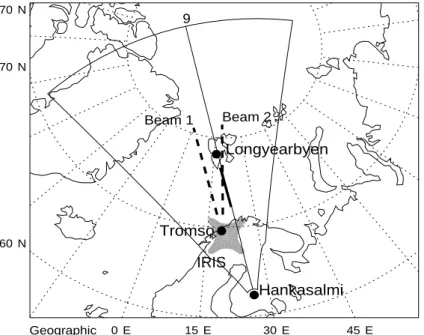
The ionospheric convection velocities in this study are pro-vided by three ionospheric radar systems, the Hankasalmi radar of the SuperDARN chain of coherent scatter HF radars (Greenwald et al., 1995), the EISCAT VHF radar at Tromsø (e.g. Rishbeth and Williams, 1985) and the EISCAT Sval-bard radar (ESR), located at Longyearbyen (e.g. Wannberg et al., 1997). The fields-of-view of these systems during the interval under study are illustrated in Fig. 1.
The SuperDARN radars form 16 beams of azimuthal sep-aration 3.24◦. Each beam is gated into 75 range bins, each of length 45 km in standard operations. During standard op-erations the dwell time for each beam is 7 s, giving a full 16 beam scan, covering 52◦in azimuth and over 3000 km in range (an area of over 4×10⁶km2), every 2 min. For the interval presented here, Hankasalmi was operating in a non-standard scan mode in which the integration time for each beam was reduced to 2 s. This reduced integration time low-ers the radar data signal-to-noise ratio slightly. The data pre-sented are thresholded as normal at 0 dB; thus, the reduced integration period reduces the data coverage, as low returned powers will be lost. In the auroral region, where powerful HF scatter is commonly observed, this has little overall effect on the data coverage. In addition to reduced integration periods, in the scan employed here, rather than the usual anticlock-wise sweep through beams 15, 14, 13,..., 0, the Hankasalmi radar scanned through the sequence 15, 9, 14, 9, 13, 9,...,1, 9, 0, 9. This allows for the construction of full 16-beam scans at an enhanced temporal resolution of 64 s, in addition to the provision of very high time resolution (4 s) data along
a single look direction (beam 9, a beam which approximately overlays the main meridional chain of the IMAGE array and the location of the ESR).
During the interval of interest, the EISCAT VHF and ESR radar systems were running the UK special programme SP-UK-CSUB. This programme was run over 4 four-hour in-tervals, commencing at 21:00 UT on 20, 21, 22 and 23 Au-gust 1998. The ESR was, during SP-UK-CSUB, directed southward, with a geographic azimuth of 161.6◦and an ele-vation of 31.0◦. This pointing direction allows for the ESR beam to be aligned in azimuth along beam 9 of the Han-kasalmi radar field-of-view. The ESR was transmitting the GUP0 radar code, a multi-frequency long pulse. Received signals were integrated over 10 s and the data subsequently analyzed at a temporal resolution of 60 s. Analysis of ESR data is such that the user can vary the range resolution, in this case with gating of 12 km below a range of 330 km, which corresponds to an altitude of around 175 km, 36 km range gates from 330 to 690 km and 72 km range gates above 690 km range; ESR observations span the altitude range from 110 to 500 km.
In SP-UK-CSUB, the EISCAT VHF radar operated in a split beam mode with one beam (beam 2) directed along the boresight which corresponds to a geographic azimuth of 359.5◦and the other (beam 1) phased 14.5◦ west to an az-imuth of 345.0◦; both beams are at an elevation of 30◦. In SP-UK-CSUB, which is identical to the VHF common pro-gramme CP-4, long pulse and power profile codes are trans-mitted. The long pulse provides observations on each beam over 20 gates of range resolution 65.3 km, with the first gate centered at a range of 533.0 km; this corresponds to an al-titude coverage from around 280 km to over 1000 km. The power profile pulse scheme yields returned power measure-ments at a range resolution of 4.5 km over 83 gates from 85 km to 285 km altitude. Like those from Svalbard, VHF observations were analyzed at 1-min temporal resolution. Beam 1 of the VHF radar is aligned in azimuth roughly along beams 6 and 7 of the Hankasalmi radar, whereas beam 2 crosses beams 7–10 of the Hankasalmi radar.
Standard analysis of the long pulse signal from both the Svalbard and VHF radars provide estimates along each beam of both ion and electron temperature, electron density and ion velocity. The VHF power profile yields estimates of electron density in the lower ionosphere. Estimates of the Hall and Pedersen conductance can be derived from the VHF power profile measurements with the incorporation of appropriate input from the MSIS-90 thermospheric model and the IGRF model of the geomagnetic field.
9
60˚N 70˚N
70˚N
0˚E 15˚E 30˚E 45˚E
Hankasalmi Tromso
Longyearbyen
Beam 1 Beam 2
Geographic
IRIS
Fig. 1. The instrumentation used in the study. The field-of-view of the Hankasalmi radar is shown, with beam 9 marked explicitly with a line. The EISCAT VHF and ESR beam positions for the SP-UK-CSUB experiment are marked with heavy lines, and the IRIS riometer field-of-view is indicated by a shaded region.
the phasing resulting in 49 narrow beams, of width between 13◦and 16◦. The beam intersections (Fig. 1) are shown at 90 km, since a large proportion of the total absorption nor-mally occurs at around this altitude. The absorption is calcu-lated by subtracting the received power from a correspond-ing quiet time power curve, and then multiplycorrespond-ing this fig-ure by the cosine of the zenith angle of the beam. The ab-sorption values attributed to the beams then represent the absorption which would have occurred if the beam passed vertically through the absorbing layer. This data set is sup-plemented here by data from ground-based fluxgate magne-tometers, provided by stations from the International Moni-tor for Auroral Geomagnetic Effects, (IMAGE) (L¨uhr, 1994). The IMAGE array has 10 s sampling for the interval under consideration here.
3 Observations
The ionospheric electric and ground magnetic fields of the substorm under study here have been presented in detail by Yeoman et al. (2000) and the reader is referred to that pa-per for a fuller discussion of the interval. A brief outline of the pertinent features is given here. Prior to 20:25 UT on 21 August 1998, the IMF, as measured by Wind, had been northward for 20 h, and the IMF By component had
been positive for 4 h. At 20:25 UT (∼20:58 UT when the features are propagated to the magnetopause), both theBy
andBzcomponents abruptly switched polarity, turning
nega-tive. The IMF remained in this configuration until 22:38 UT (∼23:11 UT at the magnetopause), when the IMFBz
com-ponent magnitude reduced to near zero, although the IMF
By component did have a brief excursion to positive values
at 21:18 UT (21:51 at the magnetopause). Some time after the IMFBzsouthward turning, at 21:40 UT, the Hankasalmi
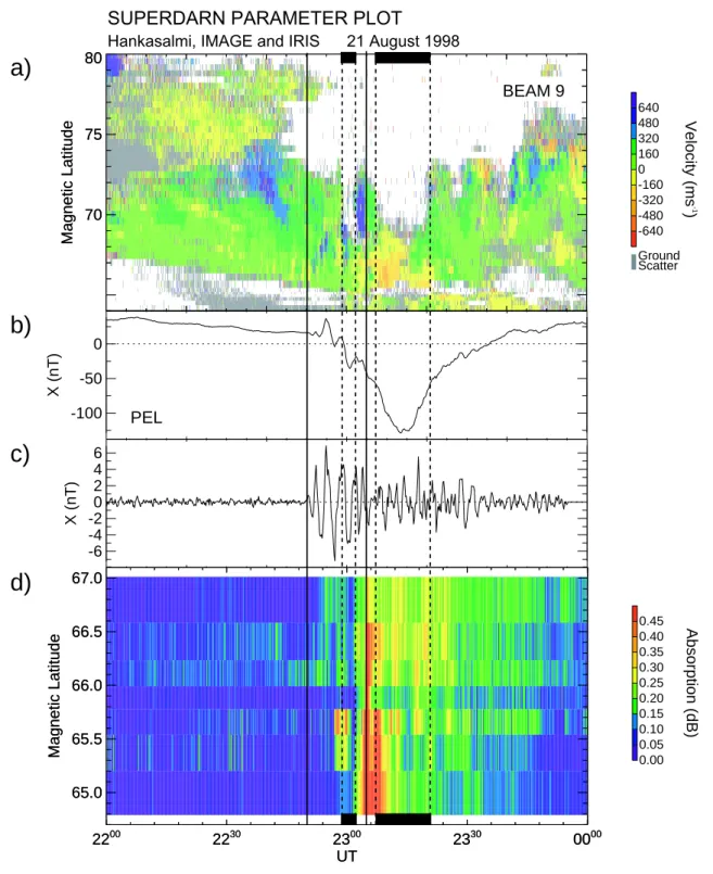
HF radar backscatter exhibited substorm growth phase signa-tures; namely an equatorward motion of the radar backscatter (Lewis et al., 1998; Yeoman et al., 1999). This is illustrated in Fig. 2a, which presents a latitude-time plot of the line-of-sight ionospheric velocities from Hankasalmi beam 9.
Magnetically quiet conditions apply up to 22:50 UT, when a clear mid-latitude Pi2 pulsation, indicating the substorm expansion phase onset is observed across the IMAGE array (the PEL station is illustrated in Fig. 2c), with a further Pi2 burst starting at 23:05 UT, which can be seen as a phase skip in the filtered PEL data, and is accompanied byY compo-nent fluctuations across the IMAGE chain (see Yeoman et al., 2000). The Pi2 onset and intensification are marked on Fig. 2 with solid vertical lines. The onset of the first Pi2 burst coincides with a strong negative bay (up to 300 nT) in theX
70 75 80
Magnetic
Latitude
70 75 80
Magnetic
Latitude
BEAM 9
-640 -480 -320 -160 0 160 320 480 640
Velocity (ms
-1
)
Ground Scatter
SUPERDARN PARAMETER PLOT
Hankasalmi, IMAGE and IRIS 21 August 1998
-100 -50 0
X (n
T
)
-6 -4 -2 0 2 4 6
X
(nT)
2200 2230 2300 2330 0000
UT 65.0
65.5 66.0 66.5 67.0
Magnetic
Latitude
2200 2230 2300 2330 0000
UT 65.0
65.5 66.0 66.5 67.0
Magnetic
Latitude
0.00 0.05 0.10 0.15 0.20 0.25 0.30 0.35 0.40 0.45 Absorption
(dB)
a)
b)
c)
d)
PEL
Fig. 2.Radar, magnetometer and riometer data for the isolated substorm under study. Pi2 onset times are marked with vertical solid lines and the intervals of HF radar data loss with vertical dashed lines.(a)Hankasalmi beam 9 line-of-sight velocity data from 22:00–24:00 UT, as a function of magnetic latitude,(b)unfilteredX(geographic north) component magnetogram from the PEL station of the IMAGE array, over the same time interval,(c)as panel b, but with a 200–20 s band-pass filter applied, in order to illustrate the Pi2 pulsation activity associated with the substorm expansion phase onset at 22:50 UT,(d)a keogram of IRIS absorption measurements from 20◦longitude.
data loss are marked on Fig. 2 with dashed vertical lines. The intervals of HF radar data loss are examined in more detail in Fig. 3. The three rows of this figure present spatial information of the HF radar backscatter power, ionospheric
on-Hankasalmi and IRIS Riometer
Power, velocity and Absorption0.00 0.06 0.12 0.18 0.24 0.30 0.36 0.42 0.48 0.54
Absorption (dB)
70˚N
15˚E
(c) 2254 00s
Geographic coordinates
(a) 2253 34s
70˚N
15˚E
0 3 6 9 12 15 18 21 24 27
Power (dB)
Geographic coordinates
(b) 2253 34s
70˚N
15˚E
-800 -600 -400 -200 0 200 400 600 800
Vel
ocity (ms
-1
)
Ground Scatter
70˚N
15˚E
(f) 2301 00s
(d) 2300 39s
70˚N
15˚E
(e) 2300 39s
70˚N
15˚E
70˚N
15˚E
(i) 2310 00s
Geographic coordinates
(g) 2308 56s
70˚N
15˚E
Geographic coordinates
(h) 2308 56s
70˚N
15˚E
70˚N
15˚E
(l) 2326 00s
Geographic coordinates
(j) 2325 32s
70˚N
15˚E
Geographic coordinates
(k) 2325 32s
70˚N
15˚E
Geographic coordinates
Geographic coordinates
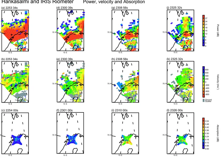
Fig. 3. Spatial distribution, in geographic coordinates, of the Hankasalmi backscatter power (top row), Hankasalmi line-of-sight velocity (middle row) and IRIS absorption (bottom row) during the substorm. The first column presents a time prior to the radar signal loss, the middle two columns present data during the signal loss period, and the final column shows the data after the radar signal has recovered.
set, during the initial period of HF radar data loss, during the second period of HF radar data loss and later on in the ex-pansion phase. Prior to the data loss, strong radar backscat-ter returns are measured, and a reasonably uniform velocity field is observed, while IRIS measures very low absorption (Figs. 3a-c). In the second column, a localized region of de-pleted radar power is observed, along with a more structured velocity field (Figs. 3d and e). A modest increase in absorp-tion is recorded by IRIS in Fig. 3f. In column three, a more spatially extensive region of HF radar data loss is observed (Fig. 3g). At this time the absorption measured by IRIS has significantly increased, reaching∼0.5 dB, and this enhanced absorption covers almost the entire IRIS field-of-view, al-though it is strongest in the southeast (Fig. 3i). Finally, in the last column, the HF radar data coverage starts to recover to values similar to Fig. 3a and the IRIS absorption reduces.
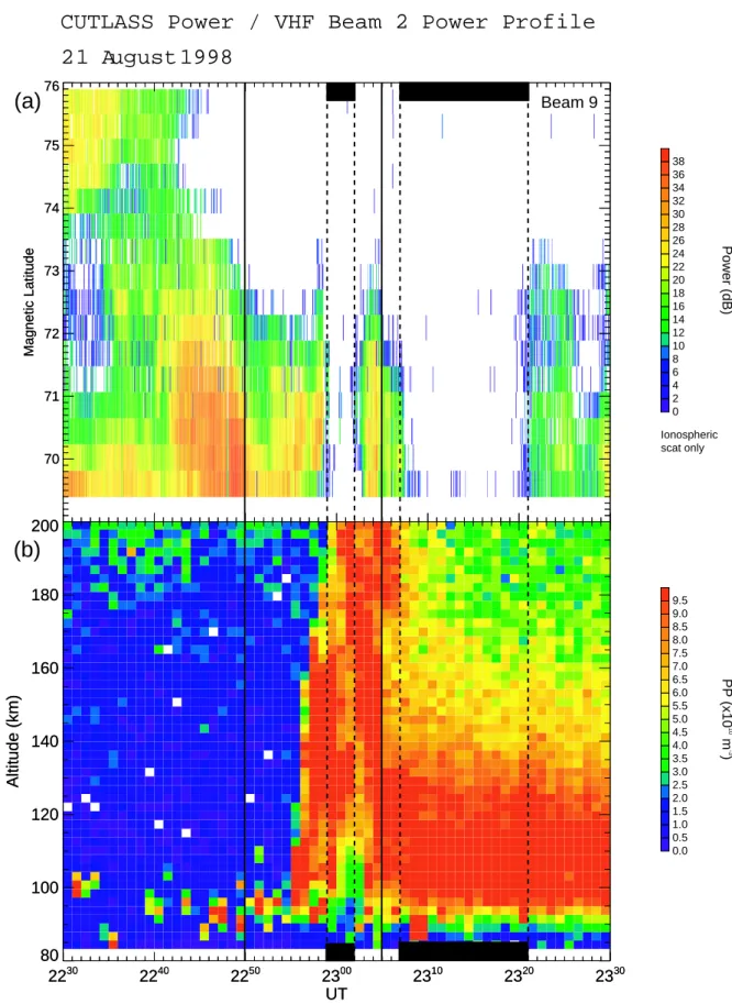
A further indication of the changing ionospheric condi-tions during the substorm interval may be obtained from the EISCAT system. Figure 4 presents Hankasalmi backscatter
70 71 72 73 74 75 76
Magnetic
Latitude
70 71 72 73 74 75 76
Magnetic
Latitude
Beam 9
0 2 4 6 8 10 12 14 16 18 20 22 24 26 28 30 32 34 36 38
Powe
r (dB)
Ionospheric scat only
2230 2240 2250 2300 2310 2320 2330
UT 80
100 120 140 160 180 200
Altitude (km
)
0.0 0.5 1.0 1.5 2.0 2.5 3.0 3.5 4.0 4.5 5.0 5.5 6.0 6.5 7.0 7.5 8.0 8.5 9.0 9.5
PP
(x10
10
m
-3
)
2230 2240 2250 2300 2310 2320 2330
UT 80
100 120 140 160 180 200
Altitude (km
)
CUTLASS Power / VHF Beam 2 Power Profile
21 August 1998
(a)
(b)
21:30 22:00 22:30 23:00 23:30 24:00 0.00
0.10 0.20 0.30 0.40
Absorption (dB)
Time (UT)
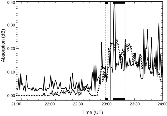
Fig. 5. Measured (dashed line) and modelled (solid line) IRIS beam 2 absorption, between 21:30 and 24:00 UT. See text for details. Pi2 onset times are marked with vertical solid lines and the intervals of HF radar data loss with vertical dashed lines, as in Fig. 2.
4 Analysis of HF propagation and absorption
4.1 Modelling IRIS absorption
The interval under study here has available both measure-ments of ionospheric absorption from IRIS, and electron den-sity profiles from EISCAT. The primary focus is to quantify the changes in HF absorption and propagation of the Han-kasalmi system using these two data sets; but first, we use the EISCAT VHF beam 2 electron density profiles from the power profile, together with an empirical atmospheric com-position and temperature model (MSIS 90), to model the ab-sorption measured by beam 2 of IRIS, which is closest to the EISCAT VHF beam 2. The absorption calculation uses the equation for the absorption coefficient given by Davies (1969), appropriate for a slowly varying plasma and nonde-viative propagation
κ=4.6·10−2
N ν
ω2+ν2
, (1)
where κ, the absorption coefficient is measured in dB/km,
N is the plasma electron density,ωis the wave angular fre-quency, andνan effective collision frequency between elec-trons and all other particles. For radio-wave absorption in the HF or VHF range, the appropriate effective collision frequen-cies are identical to the standard collision frequenfrequen-cies for mo-mentum transfer (Banks, 1966). Here electron-neutral colli-sion frequencies for N2,O2,O,H, and He from Schunk and
Nagy (1978) and the electron-ion collision frequency from Banks (1966) have been used in the absorption calculation. The values of neutral density and temperature used in the collision frequency equations are obtained from the MSIS 90 model (Hedin, 1991). The electron-neutral collision frequen-cies are actually a function of the electron temperature, but here we use the neutral temperature instead, as an approxi-mation. While the electron temperature will exceed the neu-tral temperature above 120 km, the absorption has typically fallen to 1% of its peak value at such an altitude (Davies, 1969), so this has a negligible effect on the total calculated absorption.
The absorption coefficient gives the spatial rate of change of absorption, and the total absorption,A, (in dB) is found, therefore, by integrating the absorption coefficient through distance via a summation, for a ray propagating at an angleθ
to the vertical. Although the calculated absorption assumes straight-line propagation, this does not mean that the rays penetrate the layer at a fixed angle; the Earth’s curvature con-tinually changes the effective angle at which the straight-line path passes through an assumed horizontally stratified layer, and this has been included in the calculation, which gives
A(t )=4.6·10−2
g=50
X
g=1
(h(g+1)−h(g))(secθ (h, lat, lon))
·
N (g, t )
EISCATν(h, lat, lon, t )MSIS
ω2+ν2(h, lat, lon, t ) MSIS
, (2)
0 2 4 6 0
50 100 150 200 250 300
0 2 4 6
Plasma Frequency (MHz)
0 50 100 150 200 250 300
Altitude (
km)
22:34-22:44 UT 23:07-23:17 UT
0 2 4 6
0 50 100 150 200 250 300
0 2 4 6
Plasma Frequency (MHz)
0 50 100 150 200 250 300
Altitude (km)
(a)
(b)
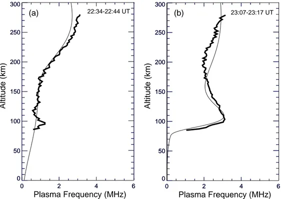
Fig. 6. Ionospheric plasma frequency profiles, derived from the EISCAT VHF beam 2. The data are indicated by the bold lines, and fitted double Chapman layers are indicated by the thin lines. (a)A profile typical of conditions prior to the substorm expansion phase onset (averaged between 22:34 and 22:44 UT).(b)A profile typical of conditions during the expansion phase (averaged between 23:07 and 23:17 UT).
altitude at the start of each range,latandlonare the latitude and longitude of each gate, N is the electron density mea-sured by EISCAT (a function of range gate and time),νis the total electron collision frequency summed over the individual expressions for each neutral species (where the neutral tem-perature and density values come from MSIS for each range gate location, and these values are combined with the appro-priate EISCAT electron density measurements in the calcula-tion), andωis the angular wave frequency of interest. Here we integrate through height (i.e.θ =90), since the absorp-tion measured by IRIS has already been normalized through division by the relative path length of the beam. On this occa-sion, the data quality beam 1 of the EISCAT VHF radar was relatively poor and could not be used for absorption calcula-tions. Beam 2 has an elevation of 30◦and azimuth 359.5◦; thus, it does not intersect with any of the IRIS beams in the main absorbing regions of around 80–90 km altitude. The 90 km ionospheric intersection of EISCAT actually occurs at a geographic latitude of 70.95◦ and a longitude of 19.13◦, making the closest beam of IRIS beam 2, which is located some 96 km to the south of this point. EISCAT has a time resolution of 1 min, and successive altitude gates are sepa-rated by 2.25 km. Absorption coefficients are assumed to be constant between each EISCAT range gate. The calculation here also requires that data exist in at least 40 of the first 50 range gates. The calculation is completed at range gate 50, an altitude of 210 km, as any contributions to the total
ab-sorption above this height are negligible.
enhance-0 5 10 15 20 25 30
Elevation angle (˚)
0 5 10 15 20
Relative absorption (dB)
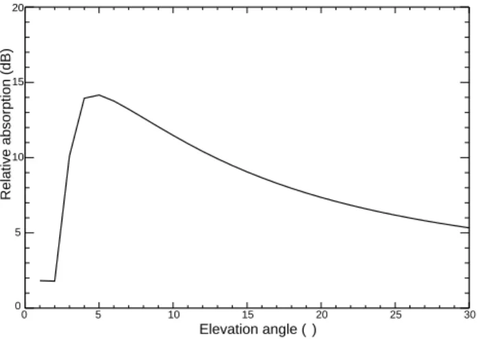
Fig. 7.A calculation of the difference in the expected absorption of the Hankasalmi HF signal before and after the substorm expansion phase onset, as a function of the radar angle-of-arrival. See text for details.
ment to the southeast is slightly delayed with respect to that in Fig. 5, due to the expanding nature of the substorm dis-turbance, but the level of absorption is of the same order as the calculated values. The similarity between the modelled and measured absorption, and the modest levels of absorp-tion measured throughout the IRIS field-of-view, suggest that the D-region absorption in this case may be approximated as a uniform absorbing region, and it is this assumption upon which the Hankasalmi absorption calculations presented in Sect. 4.2 are based.
4.2 Modelling Hankasalmi absorption
Having found a good overall correspondence between mod-elled and measured values of IRIS absorption, we apply this model to the absorption experienced by the Hankasalmi HF radar. The low EISCAT beam elevation angle means that the ionospheric electron density profiles are not measured at a single location. The resulting 1-D profiles are, however, as useful in the context of analyzing Hankasalmi absorption and HF propagation modes as 1-D profiles measured above a single geographic location; they are used merely to pro-vide an indication of the likely ray absorption and propa-gation during the substorm interval. Rather than modelling the total absorption for each available point in time, along a fixed elevation angle, as was done for IRIS, we model the total absorption as a function of the radar backscatter eleva-tion angle, using electron density profiles from two specific times, representing the conditions before substorm expan-sion phase onset and during the main interval of CUTLASS data loss during the substorm expansion phase. Figure 6a presents the EISCAT VHF beam 2 electron density profiles averaged between 22:34–22:44 UT, a time representative of the profiles from before the substorm-induced absorption en-hancement. The profile averaged between 23:07–23:17 UT (Fig. 6b) is representative of the active period, during which
the Hankasalmi data were lost. Straight-line propagation is assumed, at a range of elevation angles, using the Han-kasalmi operating frequency of 10 MHz. The assumption of straight-line propagation is chosen since the vast major-ity of the total absorption occurs in the D-region and lower E-region, at a point in the ray path where the plasma fre-quency is not high enough to cause significant refraction of a 10 MHz ray. This assumption also enables a separation of the effects of absorption and changing HF propagation con-ditions, which will be addressed in Sect. 4.3. The absorp-tion calculaabsorp-tion is again based upon Eq. (2), but now with an appropriate value ofθcalculated for each point in the sum-mation. However, the IRIS operating frequency is now re-placed by the CUTLASS operating frequency. The absorp-tion calculaabsorp-tion has been terminated when the ray reaches the ground range of Tromsø at 69.6◦ geographic latitude, a
typical range from which backscatter is received during the interval under study. Finally, the total calculated absorption is doubled since, for each ray, the backscattered radiation has passed through the absorbing layer twice (on the outward and backscattered paths).
Rather than calculate the total absorption of the Han-kasalmi HF signal, it is most useful to consider the change in absorption brought about by the substorm expansion phase onset. The change in the absorption calculated from the pro-files in Figs. 6a and b is presented in Fig. 7. The figure presents the increase in absorption associated with the sub-storm activity for rays reaching the latitude of Tromsø. A dif-ferent range termination would change the absorption profile calculated, with the range of Tromsø being chosen since it is typical for the data interval under study. Figure 7 illustrates, for a given range, how a low elevation angle path has a lower increase in absorption due to the substorm, since it propa-gates predominantly at an altitude lower than the main sorbing region, rather than within it. The peak increase in ab-sorption on the propagation path to Tromsø is just over 14 dB at an elevation angle of 5◦, with increases being smaller than 10 dB for elevation angles either greater than 15◦or less than 3◦. This level of absorption would suggest a drop in received power of at most 14 dB across the entire region in which the signal was being received, thereby resulting, in certain regions, in a complete loss of the signal. In fact, the Han-kasalmi backscattered power data presented in Figs. 3 and 4 demonstrate that some regions of the field-of-view showed the complete loss of a 30 dB signal, while neighbouring re-gions witnessed either little or no power reduction, or even in some places, an increase. This lack of consistency between prediction and observation suggests that in this case, absorp-tion is not the primary explanaabsorp-tion for the HF radar signal loss.
4.3 Modelling Hankasalmi HF propagation
100 200
300 400
500 600
700
800 900
1000 1100
1200 1300 1400
100 200 300
100 200 300
100 200
300 400
500 600
700
800 900
1000 1100 1200
1300 1400
(a)
(b)
Ground range (km)
Altitude (km)
Altit
ude
(km)
Ground range (km)
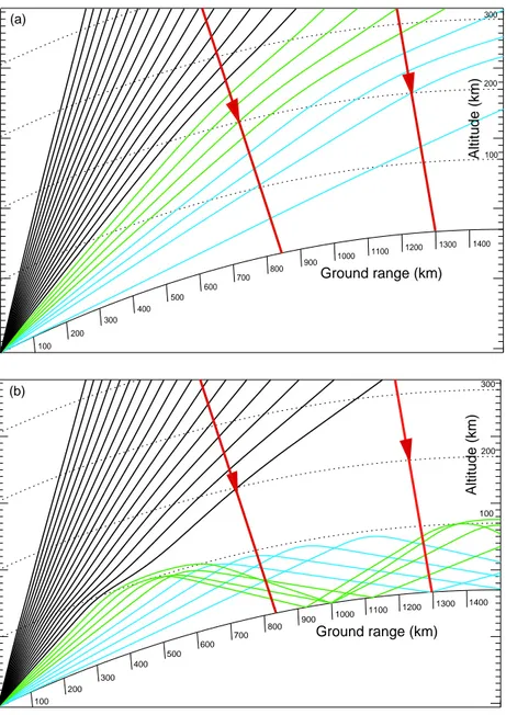
Fig. 8. A ray-tracing simulation of the HF propagation conditions for Hankasalmi(a)prior to the substorm expansion phase onset (based upon the ionospheric profile in Fig. 6a) and(b)during the substorm expansion phase (based upon the ionospheric profile in Fig. 6b). The geomagnetic field direction is indicated by the red lines. The changing HF propagation conditions affecting the HF rays indicated in black, blue and green are discussed in the text.
developed by Jones and Stephenson (1975). The ray-tracing program has been used to model radio-wave propagation at 10 MHz, the operating frequency of the CUTLASS Han-kasalmi radar, through plasma frequency profiles provided by functional fits found for the profiles measured between 22:34–22:44 UT and 23:07–23:17 UT. The form used for the fitting is the sum of two Chapman layers with the six model parameters adjusted to give the best fit. These functional fits are also shown in Figs. 6a and b. Ray trace calcula-tions through the profiles in Figs. 6a and b are displayed in Figs. 8a and b, respectively. The rays are plotted in elevation angle steps of 2◦, and range between 0◦ and 50◦. The HF propagation is thus expected to evolve from that in Fig. 8a
not strongly refracted (or indeed, absorbed) by the substorm-enhanced precipitation. In contrast, rays with elevation in the ranges 8◦–14◦(coloured green in Figs. 8a and b) are strongly refracted in Fig. 8b, and cease to be candidates for orthogonal F-region backscatter after the substorm expansion phase on-set, except at low values of ground range (∼500 km), where E-region backscatter may, in fact, be most likely. Lower el-evation angle rays (coloured blue in Figs. 8a and b) are sim-ilarly refracted, but the refraction process opens up a new HF propagation path which may sustain backscatter, with or-thogonality being achieved at ranges 800−1200 km. The rays coloured green and blue in Fig. 8 might be expected to provide ground scatter in the Hankasalmi data after the sub-storm onset. However, ionospheric scatter is expected from the same ranges, and only the scatter of the highest power will be detected. Any ground scatter will be attenuated by the requirement for the HF ray to pass through the absorbing D-region 4 times. Examination of the backscatter in Fig. 2 does reveal that some ground scatter is identified, intermingled with the dominant ionospheric scatter. This suggests that the ground scatter is of higher power than the ionospheric scatter in only a few range gates.
5 Discussion
Ionospheric radar and riometer data, combined with HF ab-sorption and propagation modelling, has been presented for an isolated substorm occurring over Scandinavia on 21 Au-gust 1998. Detailed observations of this substorm have been presented by Yeoman et al. (2000), and mid-latitude Pi2 ob-servations indicated that the substorm expansion phase on-set commenced at 22:50 UT, with a further intensification at 23:05 UT (Fig. 2). The EISCAT VHF radar detected the enhanced particle precipitation associated with the expan-sion phase onset and intensification at 22:55 and 23:04 UT, while almost simultaneously two intervals of data loss were recorded by the Hankasalmi radar, between 69◦–74◦ geo-magnetic latitude, at 22:59–23:02 UT and 23:07–23:21 UT, respectively, (Fig. 4). Such intervals of HF radar data loss are generally interpreted as resulting from HF absorption (Milan et al., 1996).
The effect of HF absorption on the Hankasalmi radar sys-tem has been addressed via a modelling calculation based upon the electron density from the power profile measured by the EISCAT VHF radar and accepted electron-neutral and electron-ion collision frequencies derived using the MSIS model. A comparison of the absorption calculated for IRIS, and the measured IRIS absorption at 38.2 MHz has demon-strated that the absorbing layer was large scale, and that a rea-sonable agreement was achieved between the measured and calculated values. Applying the same calculation, but this time to the Hankasalmi radar, operating at 10 MHz, has re-vealed that the substorm-associated precipitation is expected to produce a maximum absorption increase of ∼15 dB, at a radar elevation angle of 5◦. An examination of the mea-sured changes in Hankasalmi backscatter power, in contrast,
reveals a more variable picture, with a loss of backscatter of 30 dB or greater in some parts of the field-of-view, while elsewhere very little power is lost (Fig. 3). Therefore, it is clear that HF absorption alone is insufficient to explain the behaviour of the HF radar data during the substorm expan-sion phase.
Elevation angle (˚)
Elevation angle (˚)
0 10 20 30 40
Ground range (km)
Ground range (
km)
Occurrence
8 16 32 40 48 56 64 72
24
Occurrence
8 16 32 40 48 56 64 72
24
0 500 1000 1500 2000 0 500 1000 1500 2000
0 10 20 30 40
(b) (a)
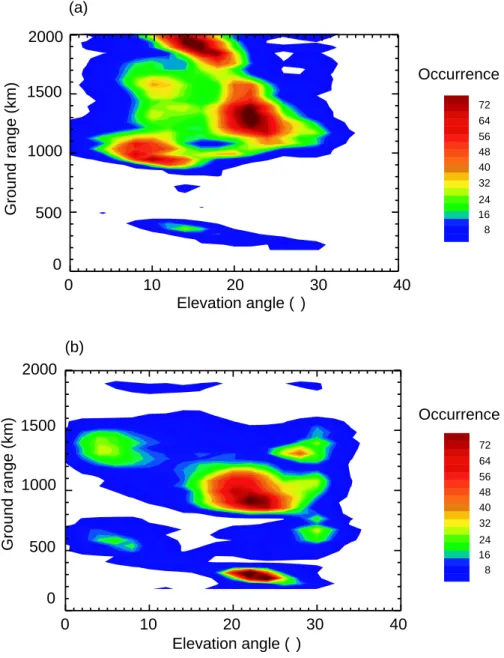
Fig. 9.The occurrence of measured Hankasalmi radar angle-of-arrival information as a function of ground range. Angle-of-arrival informa-tion from all beams of Hankasalmi are used.(a)The interval 22:20–22:50 UT, before the substorm expansion phase onset(b)The interval 22:50–23:20 UT, during the substorm expansion phase.
Fig. 8b, are both viable new propagation paths for HF radar backscatter. The total amount of backscatter recorded is also clearly reduced between Figs. 9a and b. These changes in received backscatter elevation angles are largely consis-tent with the ray-tracing analysis presented in Fig. 8. This suggests that the changes in, and losses of, backscatter at substorm onset were primarily a consequence of altered HF propagation conditions. The substorm precipitation resulted in a region of modest absorption increase of a scale size sim-ilar to the IRIS field-of-view. HF propagation conditions in this region were significantly altered, with a new, low eleva-tion angle propagaeleva-tion path opening up in the region of the substorm-affected ionosphere.
ve-70 71 72 73 74
Magnetic Latitude
70 71 72 73 74
Magnetic Latitude
1 km/s
2230 2240 2250 2300 2310 2320 2330
UT 0
5 10 15 20 25
H
all Conductance (S)
Beam 2, Az: 359.5 El: 30.0 70
71 72 73 74
Magnetic
Latitude
-640 -480 -320 -160 0 160 320 480 640
V
e
locity (ms
-1
)
70 71 72 73 74
Magnetic
Latitude
SP-UK-CSUB
21 August 1998(a)
(b)
(c)
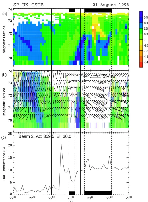
Fig. 10. (a)Line-of-sight velocity measurements from the ESR, as a function of magnetic latitude, for the interval 22:30–23:30 UT. Pi2 onset times are marked with vertical solid lines and the intervals of HF radar data loss with vertical dashed lines, as in Fig. 2. (b)Hankasalmi beam 9 measurements of line-of-sight velocity for the same times and latitudes as panel (a). Overlayed are estimates of the convection velocity, derived from a beam-swinging analysis of data from beams 1 and 2 of the EISCAT VHF system. (c)An estimate of the Hall conductance derived from data measured in the beam 2 direction of the EISCAT VHF system.
locities, visible in the Hankasalmi line of sight data presented in Figs. 2 and 10 after 22:55 UT. Clearly, as Hankasalmi suf-fers from data loss shortly after this time, it is not an ideal instrument to characterize the velocity field. However, the EISCAT radars do not suffer from such a data loss, and can provide independent velocity measurements where the EIS-CAT beams are close to being collocated with Hankasalmi beam 9. Both the EISCAT VHF Tromsø radar and the
over-laid with velocity vectors derived from the VHF beams 1 and 2, calculated via a beam-swinging technique. Finally, Fig. 10c presents the Hall conductance derived from the VHF beam 2 power profile equatorward of the velocity measure-ments. The Pi2 onset times are marked with vertical solid lines and the intervals of HF radar data loss with vertical dashed lines, as in Fig. 2. An increase in energetic parti-cle precipitation, as evidenced from the enhanced Hall con-ductance, peaks at 22:55 UT, and persists at a lower, but still enhanced level thereafter. The initial Hankasalmi data loss interval can be seen to coincide with an interval of reduced ionospheric convection velocity, whereas the convection is strong for the second interval, in spite of the conductivity in-crease. A possible consequence of such an electric field sup-pression is the reduction of ionospheric irregularities in the low electric field region (Milan et al., 1999). The increasing strength of the equatorward flows at 23:02 UT indicate the return of the Hankasalmi data. Subsequent to this feature an extended data gap appears in the Hankasalmi data, after the electric field has recovered, but also after the substorm pre-cipitation has significantly altered the HF propagation condi-tions. The likelihood that irregularities would have been lost during the substorm interval due to reduced electric fields has so far been neglected, and of course, the level of scattering structure present at any particular time and place cannot be easily assessed. The best evidence that one can obtain simply in support of there being an effective depletion in scattering structure is to show that the electric field strength and radar power have been reduced simultaneously in a particular lo-cation. This is the case in Fig. 10, and suggests that electric field reduction plays some role in the initial, short-lived in-terval of HF radar data loss.
6 Summary
Data from the Hankasalmi HF radar, the EISCAT incoher-ent scatter radars and the IRIS riometer, combined with cal-culations of HF absorption and propagation have enabled a quantitative insight to be gained into the operational con-straints put upon HF radar systems by changes in the iono-sphere associated with substorm precipitation. While large substorm expansion phase onsets local to the radar field-of-view would result no doubt in the complete absorption of the SuperDARN HF radar signal, we have demonstrated that for smaller events the radars are able to receive backscatter in spite of riometer absorption levels of∼0.5 dB at 38 MHz. A more significant constraint is presented by the changing HF propagation conditions, which can result in the loss of viability of HF rays of certain elevation angles as candidates for HF backscatter. In contrast, new, very low elevation an-gle backscatter HF propagation paths are opened up by the substorm precipitation. SuperDARN radars are frequency agile between 8 and 20 MHz, so careful frequency manage-ment, when combined with ray-tracing simulations such as that presented in Fig. 8, may significantly improve data cov-erage during the substorm expansion phase. In addition, the
HF radar data loss may be used to track the location and prop-agation of the enhanced regions of D-region absorption, and to evaluate the modifications to the available HF propagation paths which are imposed on HF communications links by the localized regions of the auroral ionosphere affected by substorm precipitation. In addition, it is suggested that for brief intervals during the substorm expansion phase that the suppression of the ionospheric electric field can contribute to the loss of HF radar backscatter, via a reduction in the ionospheric irregularities responsible for forming the radar targets.
Acknowledgements. The CUTLASS HF radars are deployed and operated by the University of Leicester, and are jointly funded by the UK Particle Physics and Astronomy Research Council (Grant no. PPA/R/R/1997/00256), the Finnish Meteorological Institute, and the Swedish Institute for Space Physics. The authors thank the director and staff of EISCAT for the operation of the facility and dissemination of the data. EISCAT is an international facil-ity funded collaboratively by the research councils of Finland (SA), France (CNRS), the Federal Republic of Germany (MPG), Japan (NIPR), Norway (NAVF), Sweden (NFR) and the United Kingdom (PPARC). IMAGE data were kindly supplied by the Finnish Mete-orological Institute. JKG was supported by a PPARC studentship. JAD is supported on PPARC Grant number PPA/G/O/1997/000254. The riometer data originated from the Imaging Riometer for Iono-spheric Studies (IRIS), operated by the Department of Communica-tions Systems at Lancaster University (UK), funded by the Particle Physics and Astronomy Research Council (PPARC) in collabora-tion with the Sodankyl¨a Geophysical Observatory.
The Editor in chief thanks G. Chisham for his help in evaluating this paper.
References
Baker, K. B., and Wing, S.: A new magnetic coordinate system for conjugate studies at high-latitudes, J. Geophys. Res., 94, 9139– 9143, 1989.
Banks, P. M.: Collision frequency and energy transfer: Ions, Planet. Space Sci. 14, 1105–1122, 1966.
Baumjohann, W., Pellinen, R. J., Opgenoorth, H. J., and Nielsen, E.: Joint two-dimensional observations of ground magnetic and ionospheric electric fields associated with auroral zone currents: current systems associated with local auroral break-ups, Planet. Space. Sci., 29, 431–447, 1981.
Browne, S., Hargreaves, J. K., and Honary, F.: An imaging riome-ter for ionospheric studies, Electronics and Communication En-gineering Journal 7, 209–217, 1995.
Davies, J. A., Yeoman, T. K., Lester, M., and Milan, S. E.: A com-parison of F-region ion velocity observations from the EISCAT Svalbard and VHF radars with irregularity drift velocity mea-surements from the CUTLASS Finland HF radar, Ann. Geophys-icae, 18, 589–594, 2000.
Davies, K.: Ionospheric Radio, Blaisdell Publishing Company, USA, 1969.
Darn/Superdarn: A global view of the dynamics of high-latitude convection, Space Sci. Rev., 71, 761–796, 1995.
Hedin, A. E.: Extension of the MSIS thermosphere model into the middle and lower atmosphere, J. Geophys. Res. 96, 1159–1172, 1991.
Inhester, B., Baumjohann, W., Greenwald, R. A., and Nielsen, E.: Joint two-dimensional observations of ground magnetic and ionospheric electric fields associated with auroral zone currents 3. Auroral zone currents during the passage of a westward trav-elling surge, J. Geophys., 49, 155–162, 1981.
Jones, R. M. and Stephenson, J. J.: A versatile three-dimensional ray-tracing computer program for radio waves in the ionosphere, OT Report 75–76, US Govt. Printing Office, Washington DC, 1975.
Lester, M., Milan, S. E., Besser, V., and Smith, R.: A case study of HF radar spectra and 630.0 nm auroral emission in the pre-midnight sector, Ann. Geophysicae, 19, 327–339, 2001. Lewis, R. V., Freeman, M. P., and Reeves, G. D.: The relationship of
HF radar backscatter to the accumulation of open magnetic flux prior to substorm onset, J. Geophys. Res., 103, 26 613–26 619, 1998.
Lewis, R. V., Freeman, M. P., Rodger, A. S., Reeves, G. D., and Milling, D. K.: The electric field response to the growth phase and expansion phase onset of a small isolated substorm, Ann. Geophysicae, 15, 289–299, 1997.
L¨uhr, H.: The IMAGE magnetometer network, STEP International Newsletter, 4, no. 10, 4–6, 1994.
Milan, S. E., Davies, J. A., and Lester, M.: Coherent HF radar backscatter characteristics associated with auroral forms identi-fied by incoherent radar techniques: a comparison of CUTLASS and EISCAT observations, J. Geophys. Res., 104, 22 591–22 604, 1999.
Milan, S. E., Jones, T. B., Lester, M., Warrington, E. M., and Reeves, G. D.: Substorm correlated absorption on a 3200 km trans-auroral HF propagation path, Ann. Geophys., 14, 182–190, 1996.
Morelli, J. P., Bunting, R. J., Cowley, S. W. H., Farrugia, C. J., Freeman, M. P., Friis-Christensen, E., Jones, G. O. L., Lester, M., Lewis, R. V., L¨uhr, H., Orr, D., Pinnock, M., Reeves, G. D., Williams P. J. S., and Yeoman, T. K.: Radar observa-tions of auroral zone flows during a multiple-onset substorm, Ann.Geophysicae, 13, 1144–1163, 1995.
Opgenoorth, H. J., Bromage, B., Fontaine, D., LaHoz, C., Huusko-nen, A., Kohl, H., Løvhaug, U.-P., Wannberg, G., Gustaffson, G., Murphree, J. S., Eliasson, L., Marklund, G., Potemra, T. A., Kirkwood, S., Nielsen, E., and Wahlund, J.-E. Coordinated ob-servations with EISCAT and the Viking satellite: the decay of a westward travelling surge, Ann. Geophyicae, 7, 479–500, 1989. Rishbeth, H. and Williams, P. J. S.: The EISCAT ionospheric radar:
The system and its early results Q. J. R. Astr. Soc., 26, 478–512, 1985.
Robinson, T. R.: Towards a self-consistent nonlinear theory of radar-auroral backscatter, J. Atmos. Terr. Phys., 48, 417–422, 1986.
Schunk, R. W. and Nagy, A. F.: Electron temperatures in the F-region of the ionosphere: Theory and observations, Rev. Geo-phys. Space Phys. 16, 355–399, 1978.
Shand, B. A., Yeoman, T. K., Lewis, R. V., Greenwald, R. A., and Hairston, M. R.: Inter-hemispheric contrasts in the ionospheric convection response to changes in the Interplanetary Magnetic Field and substorm activity: A case study, Ann. Geophysicae, 16, 764–774, 1998.
Wannberg G., Wolf, L., Vanhainen, L.-G., Koskenniemi, K., R¨ottger, J., Postila, M., Markkanen, J., Jacobsen, R., Stenberg, A., Larsen, R., Eliassen, S., Heck S., and Huuskonen, A.: The EISCAT Svalbard radar: a case study in modern incoherent scat-ter radar system design, Radio Science, 32, 2283–2307, 1997. Yeoman, T. K. and L¨uhr, H.: CUTLASS/IMAGE observations of
high-latitude convection features during substorms, Ann. Geo-physicae, 15, 692–702, 1997.
Yeoman, T. K., Davies, J. A., Wade, N. M., Provan, G., and Milan, S. E.: Combined CUTLASS, EISCAT and ESR observations of ionospheric plasma flows at the onset of an isolated substorm, Ann. Geophysicae, 18, 1073–1087, 2000.
Yeoman, T. K., Lewis, R. V., Milan, S. E., and Watanabe, M.: An interhemispheric study of the ground magnetic and ionospheric electric fields during the substorm growth phase and expansion phase onset, J. Geophys. Res., 104, 14 867–14 877, 1999. Yeoman, T. K., Mukai, T., and Yamamoto, T.: Simultaneous