Forecasting the Portuguese stock market time series by using artificial neural networks

(1)

This content has been downloaded from IOPscience. Please scroll down to see the full text.

Download details:

IP Address: 193.136.189.2

This content was downloaded on 26/06/2015 at 11:49

Please note that terms and conditions apply.

Forecasting the portuguese stock market time series by using artificial neural networks

View the table of contents for this issue, or go to the journal homepage for more 2010 J. Phys.: Conf. Ser. 221 012017

(http://iopscience.iop.org/1742-6596/221/1/012017)

(2)

Forecasting the Portuguese Stock Market Time Series by

Using Artificial Neural Networks

Monica Isfan1, 2, Rui Menezes3 and Diana A. Mendes3

1

Department of Statistical Metodology, INE, Avenida António José de Almeida, 1000-043 Lisbon, Portugal

2

ISCTE-IUL, Avenida das Forças Armadas, 1649-026 Lisbon, Portugal 3

Department of Quantitative Methods, ISCTE-IUL and UNIDE, Avenida das Forças Armadas, 1649-026 Lisbon, Portugal

E-mail: monica.isfan@ine.pt; rui.menezes@iscte.pt and diana.mendes@iscte.pt

Abstract. In this paper, we show that neural networks can be used to uncover the non-linearity that exists in the financial data. First, we follow a traditional approach by analysing the deterministic/stochastic characteristics of the Portuguese stock market data and some typical features are studied, like the Hurst exponents, among others. We also simulate a BDS test to investigate nonlinearities and the results are as expected: the financial time series do not exhibit linear dependence. Secondly, we trained four types of neural networks for the stock markets and used the models to make forecasts. The artificial neural networks were obtained using a three-layer feed-forward topology and the back-propagation learning algorithm. The quite large number of parameters that must be selected to develop a neural network forecasting model involves some trial and as a consequence the error is not small enough. In order to improve this we use a nonlinear optimization algorithm to minimize the error. Finally, the output of the 4 models is quite similar, leading to a qualitative forecast that we compare with the results of the application of k-nearest-neighbor for the same time series.

1. Introduction

Time series analyses and in particular forecasting of financial data have attracted some special attention in the last years. Unfortunately, the nonlinear nature and the complex behaviour of this type of data transform forecasting into a very hard task, and the classical statistical methods turn to be not adequate. A new generation of methodologies, including artificial neural networks (ANN) and genetic algorithms (GA) has been used for the analysis of trends and patterns, classification and forecasting. In particular, the use of computational intelligence based techniques for forecasting has proved to be extremely successful in recent times due to the ability of neural networks to approximate nonlinear functions [2, 8, 13, 14, 16, 20, 21].

Stock market prediction is very difficult. The efficient market hypothesis states that the current market price fully reflects all available information. This implies that past and current information is incorporated into stock price, thus price changes are merely due to new information and irrelevant to existing information. Since news occur randomly and cannot be forecasted, stock price should follow a random walk pattern. If this hypothesis is true, then any attempts to predict market will be futile. The random walk model has been tested extensively in various markets. The results are mixed and

7th International Conference on Applications of Physics in Financial Analysis IOP Publishing Journal of Physics: Conference Series 221 (2010) 012017 doi:10.1088/1742-6596/221/1/012017

(3)

sometimes contradictory. However, most of the recent studies [6, 7, 8, 10, 16, 17] on stock markets reject the random walk behavior of stock prices. Although numerous reports produce evidence that stock prices are not purely random, they all agree that the behavior of stock prices is approximately close to a random walk process.

Moreover, if the underlying process to a market time series is a fractional random walk, which can be deduced by estimating the Hurst exponent, then the only methods available for prediction are the neural algorithms [16, 18].

An artificial neural network is a mathematical model or a computational model based on biological neural networks or, in other words, is an emulation of a biological neural system. It consists of an interconnected group of artificial neurons and processes information using a connectionist approach to computation. The ANN is a powerful tool for nonlinear time series models and, in the last years, was used with success in solving nonlinear prediction and forecasting problems. In particular, ANNs are used to forecast financial markets, since they are able to learn nonlinear mappings between inputs and outputs, the systems' model is no needed (no priori assumption is needed) and can be applied to no-stationary data. Neural network forecasting models have been widely used in financial time series analysis during the last decade [2, 7, 13, 14, 15, 18, 20, 21].

In this paper, we show that neural networks can be used to uncover the non-linearity that exists in the financial field. First, we follow a traditional approach by analysing some of the deterministic/stochastic characteristics of the Portuguese stock exchange index and some typical features are done. We also produce a BDS (Brock, Dechert, and Scheinckman, 1987) test to investigate the nonlinearity and the result was as expected: the financial time series do not exhibit linear dependence. We analyze several periods with large and small Hurst exponents in order to obtain indications to make efficient the process of prediction time series with a multi-layer ANN with supervised learning. Secondly, we trained four types of neural networks for the stock markets and used the models to make a forecast.

ANN models were obtained using a three-layer feed-forward topology and the back-propagation learning optimization algorithm. The quite large number of parameters that must be selected to develop a neural network forecasting model involves some trial and as a consequence the error is not small enough. In order to improve this we use some nonlinear optimization numerical algorithm to minimize the error. Finally, the output of the 4 models was quite similar, leading to a qualitative forecast.

To compare the forecast errors for the above considered cases; we also forecast the data by using nearest neighborhood methods. By analyzing the response of various configurations to our data series, with specific characteristics; we conclude that the forecasting results when neural networks are applied are better than k-nearest-neighbor forecast results.

Nearest neighbor forecasting models are attractive with their simplicity and the ability to predict complex nonlinear behavior. They rely on the assumption that observations similar to the target one are also likely to have similar outcomes. A common practice in nearest neighbor model selection is to compute the globally optimal number of neighbors on a validation set, which is later applied for all incoming queries. For certain queries, however, this number may be suboptimal and forecasts that deviate a lot from the true realization could be produced.

2. Methodology

Formally, the problem of prediction of future values of some time series y(t), t = 1,2,…, can be formulated as finding a (nonlinear) function F so as to obtain an estimate y’(t + D) of the vector y at

(4)

time t+D (D = 1,2, …), given the values of y up to time t, plus a number of additional time independent variables (exogenous features) ui:

y’ (t+D) =F(y(t), … y(t-dy), u(t), …, u(t-du)),

where u(t) and y(t) represent the input and output of the model at time t, du and dy are the lags of the input and output of the system and F a nonlinear function. Typically, D = 1, means one-step ahead, but we can take any value larger than 1 and we say multi-step ahead prediction.

Viewed this way, prediction becomes a problem of (nonlinear) function approximation, where the purpose of the method is to approximate the continuous function F as closely as possible.

Usually, the evaluation of prediction performance is done by computing an error measure E over a number of time series elements, such as a validation or test set:

E=∑ (y’ (t-k) y (t-k))

E is a function measuring the error between the estimated (predicted) and actual sequence element.

Typically, a distance measure (Euclidean or other) is used, but depending on the problem, any function can be used.

The adopted methodology in this work is based on three main steps: firstly, we established the architecture for the ANN; in particular a multilayer feed-forward artificial neural network with supervised training realized through the back-propagation algorithm. The error function was optimized by a numerical optimization technique based on Levenberg-Marquard algorithm. Secondly, in order to test the forecasting ability we due some basic descriptive statistics of the data and estimate the Hurst exponents. Finally, we forecast the future values for the Portuguese stock exchange (index) time series by using ANN and nearest neighbour with correlation and with absolute distance.

2.1. Feed-forward Artificial Neural Networks

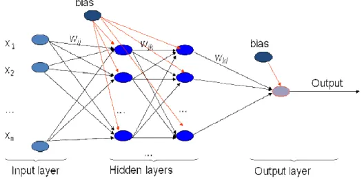
Feed-forward neural networks [13], [15] are the simplest form of ANN. A feed-forward neural network (figure 1) is a biologically inspired classification algorithm. It consists of a (possibly large) number of simple neuron-like processing units, organized in layers. Every unit in a layer is connected with all the units in the previous layer. These connections are not all equal; each connection may have a different strength or weight. The weights on these connections encode the knowledge of a network and the transformation of the node information is realized by the activation function.

Data enters at the inputs and passes through the network, layer by layer, until it arrives at the

outputs. During normal operation, that is when it acts as a classifier, there is no feedback

between layers. This is why they are called feed-forward neural networks.

(5)

Figure 1. Feed-forward artificial neural network

Training an artificial neural network involves presenting input patterns in a way so that the system minimizes its errors and improves its performance. The training algorithm may vary depending on the network architecture, but the most common training algorithm used is back-propagation [6], [10]. This is the process of back-propagating errors through the system from the output layer towards the input layer during the training (figure 2). Back-propagation is necessary because hidden units have no training target value that can be used, so they must be trained based on errors from previous layers. The output layer is the only layer which has a target value which can be compared. As the errors are back-propagated through the nodes, the connection weights are changed. Training occurs until the errors in the weights are sufficiently small to be accepted.

Back-propagation algorithms are often too slow for practical problems, so we can use several high performance algorithms [9]. These faster algorithms fall into two main categories: heuristic techniques (as variables learning rate back-propagation, resilient back-propagation) and numerical optimization techniques (as conjugate gradient, Levenberg-Marquardt, etc.). In this paper, Levenberg-Marquardt algorithm, the sigmoid transfer function in the hidden layer and a linear transfer function in the

output layer were suitable for our study.

The major problem in training an ANN is deciding when to stop training. Since the ability to generalize is fundamental for these networks to predict future values, overtraining is a serious problem. Overtraining occurs when the system memorize patterns and thus looses the ability to generalize. Overtraining can occur by having too many hidden nodes or training for too many time periods (epochs). However, overtraining can be prevented by performing test and train procedures or cross-validation. The test and train procedure involves training the network on most of the input data (around 90%) and testing on the remaining data. The network performance on the test set is a good indicator of its ability to generalize and handle data it has not been trained on. If the performance on the test is poor, the network configuration or learning parameters can be changed. The network is then retrained until its performance is satisfactory.

(6)

Figure 2. Backpropagation algorithm

2.2. Hurst exponent

In time series forecasting, the first question we want to know is whether the data under study is predictable. If the time series is random, then all methods are expected to fail. For this reason, we need some more details about the data, and we try to identify and study those time series having at least some degree of predictability.

The Hurst exponent, proposed by H. E. Hurst [10] for use in fractal analysis, has been applied to many research fields, and recently in finance domain. The Hurst exponent provides a measure for long-term memory and fractality of a time series and in consequence, can be used as a numerical estimate of the predictability of a time series. It is defined as the relative tendency of a time series to either regress to a longer term mean value or cluster in a direction. The reason the Hurst Exponent is an estimate and not a definitive measure is because the algorithm operates under the assumption that the time series is a pure fractal, which is not entirely true for most financial time series.

In conjunction with technical indicators or neural networks, Hurst Exponent estimation can help to determine which assets to forecast and which ones to ignore. This can be particularly useful in neural nets where models can focus more on time series with higher predictability. The date period is usually chosen arbitrary without any explanations. In this paper, we use the Hurst exponent to select period with great predictability to do further investigation.

The Hurst exponent [18] can be calculated by rescaled range analysis (R/S analysis). Hurst find that (R/S) scales by power-law as time increases, which indicates

(R/S)t =ct H

(1)

where R is the range series, S is the standard deviation series, (R/S) is the rescaled range series, c is a constant and H is the Hurst exponent.

The values of the Hurst exponent range between 0 and 1. Based on the Hurst exponent value H, a time series can be classified into three categories:

• H=0.5 indicates a random series;

• 0<H<0.5 indicates an anti-persistent series;

(7)

• 0.5<H<1 indicates a persistent series.

An anti-persistent series has characteristics of "mean-reverting", which means an up value is more likely followed by a down value, and vice-versa. The strength of "mean-reverting" increases as H approaches 0.0. A persistent series is trend reinforcing, which means the direction of the next value is more likely the same as current value. The strength of trend increases as H approaches 1.0. Most economic and financial series are persistent with H>0.5. To estimate the Hurst exponent, we plot (R/S) versus t in log-log axes. The slope of the regression line approximates the Hurst exponent.

2.3. Nearest neighbour algorithm

The k-nearest neighbour (k-NN) algorithm is defined as a non-parametric regression. In order to obtain some forecast, we first have to identify the k most similar time series to a given query and then, by combining their historical continuations, evaluate the expected outcome for the query. For the k-NN the location of the observation in time is not important, because the objective of the algorithm is to locate similar pieces of information, independently of the respective time location. Thus the main idea of k-NN is to capture a non-linear dynamic of self similarity of the series.

The methods are linear with respect to the model parameters, and yet they turn out to be suitable for predicting highly nonlinear fluctuations too. This is due to the fact that the identified neighbors themselves could comprise complex nonlinear patterns.

The univariate nearest neighbour correlation method. The univariate case for k-NN algorithm [4, 5]

works with the following steps:

• We define a starting training period and divide the period on different sectors or pieces yt m

of

size m, where t=m,...,T and T is the number of observation on the training period. The term m is also defined as the embedding dimension of the time series. The last sector available before the observation to be forecast will be called yTm, and the other pieces will be called yim.

• We select k pieces most similar to yT m

. For the method of correlation, that means that we search for the k pieces with the highest value of |q|, which represents the absolute correlation between yi

m

and yT

m

.

• With k pieces on hand (each one with m observations), is necessary to understand in which way the k vectors can be used to construct the forecast on (t+1). Several methods can be considered here, including the use of an average or of a tricube function.

The univariate nearest neighbour absolute distance method. The method of absolute distance [4, 5] is

much simpler than the method of correlation, and the steps to follow are:

• We define a starting training period and divide the period on different sectors or pieces yt m

of

size m, where t=m,...,T and T is the number of observation on the training period. The term m is also defined as the embedding dimension of the time series. The last sector available before the observation to be forecast will be called yT

m

, and the other pieces will be called yi m

. • We select k pieces most similar to yT

m

. For the method of absolute distance, that means that we search for the k pieces with the lowest sum of distances between the vectors yi

m

and yT

m

.

• With k pieces on hand (each one with m observations), is necessary to understand in which way the k vectors can be used to construct the forecast on (t+1). The absolute distance method simply verifies the observations ahead of the k chosen neighbours and takes the average of them.

3. Data

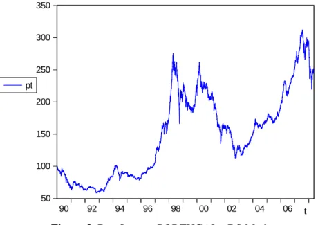
The input variables are given by the Portuguese stock exchange market and consist of 4789 daily observations; 5 days per week (see figure 3). The data is non-stationary, with high skewness and kurtosis, and non-normal distribution, as can be observed from figure 4.

(8)

The BDS statistics clearly shows that there is no linear dependence in the data (see table 1). The BDS test tests the null hypothesis of independent and identical distribution (i.i.d.) in the data against an unspecified departure from i.i.d. A rejection of the i.i.d. null hypothesis in the BDS test is consistent with some type of dependence in the data, which could result from a linear stochastic system, a nonlinear stochastic system, or a nonlinear deterministic system. Under the null hypothesis, the BDS test statistic asymptotically converges to a standard normal distribution.

In table 1, C(m,n) corresponds to the correlation integral, m is the embedding dimension and n the distance between the standard deviation of the data.

We applied the BDS test to our data for embedding dimensions of m = 2,3,4,5 and 6. We use the quantiles from the small sample simulations reported by Brock et al. [1] as approximations to the finite-sample critical values of our BDS statistics. The i.i.d. null hypothesis is rejected in all cases for yield changes.

The data were divided into two sets, the training set and the test set (3831 observation were used for the training of the network while the rest of 958 data was used for testing). The Hurst exponent, ANN models and k-NN prediction were analyzed and estimate by using MATLAB packages and programs. The out-of-sample forecasting horizon is one-step ahead, with the competing forecasting models estimated over the training set and applied over the test set to generate genuine one-step-ahead out-of-sample forecasts. The criterion for forecasting performance is absolute mean.

The analysis was initially done for the original non-stationary data and after extended to the log difference data. We stress out that all the initial parameters and the algorithms implemented are the same for the original data and log difference data.

50 100 150 200 250 300 350 90 92 94 96 98 00 02 04 06 pt t

Figure 3. DataStream: PORTUGAL - DS Market

(9)

0 100 200 300 400 500 600 80 120 160 200 240 280 320 Series: PT Sample 1/02/1990 5/12/2008 Observations 4790 Mean 149.5132 Median 151.5150 Maximum 312.1800 Minimum 58.83000 Std. Dev. 66.51653 Skewness 0.384446 Kurtosis 2.054050 Jarque-Bera 296.5841 Probability 0.000000

Figure 4. DataStream: PORTUGAL - DS Market Table 1. BDS statistics for Portuguese Stock Market

4. Results

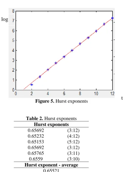
We do several tests in order to estimate the Hurst exponent, for the considered data. As we can observe from figure 5 and table 2 the average Hurst exponent we found is approximately equal to 0.65, meaning that the time series is trend reinforcing. This indicates that we are in the presence of a long memory dependence process with low fractal dimensions and in consequence the date is quite predictable.

(10)

Figure 5. Hurst exponents

Table 2. Hurst exponents Hurst exponents 0.65692 (3:12) 0.65232 (4:12) 0.65153 (5:12) 0.65692 (3:12) 0.65765 (3:11) 0.6559 (3:10)

Hurst exponent - average 0.65521

In all the performed simulations and estimations, a one-step-ahead prediction is considered; that is, the actual observed values of all lagged samples are used as inputs.

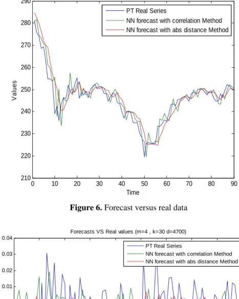
In figure 6 and figure 7, respectively we have represented the real no-stationary data versus the forecasted data by using nearest neighbour with correlation and with absolute distance methods and the log difference data versus the forecasted data using the same methods as above. For the two forecast algorithms (nearest neighbour with correlation method and absolute distance method) and for both original data and log difference data, we considered

4700 observations on the training period, k= 30 most similar pieces and m=4 the embedding

dimension. The results for the absolute mean error and correlation mean error are showed in table 3.

Table 3. Absolute mean error and correlation mean error

Mean absolute error Correlation mean error

Real data 1.0245 0.7819

Log difference data 1.8993e-004 8.1925e-004

t

log

(11)

0 10 20 30 40 50 60 70 80 90 210 220 230 240 250 260 270 280 290 Time V a lu e s

Forecasts VS Real values (m=4 , k=30 d=4700) PT Real Series

NN forecast with correlation Method NN forecast with abs distance Method

Figure 6. Forecast versus real data

0 10 20 30 40 50 60 70 80 90 -0.06 -0.05 -0.04 -0.03 -0.02 -0.01 0 0.01 0.02 0.03 0.04 Time V a lu e s

Forecasts VS Real values (m=4 , k=30 d=4700) PT Real Series

NN forecast with correlation Method NN forecast with abs distance Method

Figure 7. Forecast versus log difference data

We can observe that, for this forecasting method, we obtain better results if we apply the methods to the stationary log difference data, than for the non-stationary data.

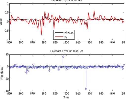
In figure 8 and 9 we illustrate the forecast results for the original and respectively, the log

(12)

difference data and the forecast of the error for the test set.

Various ANN models with different numbers of lagged input steps (or time windows), and different number of neurons in hidden layers have been compared. All the models had layer 1 (input) with N neurons and a single neuron in layer 2 (output layer). The main characteristics for our optimal ANN are registered in Table 4, namely the best performance was obtained for a 3-layer feed-forward neural network with 12 hidden units, low learning rate (0.1) and trained for maximum 2000 epochs. In order to obtain fast convergence we apply the Levenbeg-Marquardt algorithm.

850 860 870 880 890 900 910 920 930 940 950 0.2 0.4 0.6 0.8 1 v al ue

Frecasted by Optimal Net

yhatopt yy 850 860 870 880 890 900 910 920 930 940 950 -0.2 -0.1 0 0.1 0.2 0.3 Time R es idul as

Forecast Error for Test Set

Figure 8. Forecast of original data by the optimal ANN

In figure 8 yy is the original data and yhatopt represents the forecast results for original data. In figure 9, yy stands for the log difference data and yhatopt represents the forecast results for log difference data.

We can observe in this case that ANN methods perform a better prediction for the original

no-stationary data than for the log difference data. We also highlight, that we obtain a lower forecast error for stationary log difference data by using k-nearest neighbour.

Consequently, the use of ANN provides fast convergence, high precision and strong forecasting ability of real data. Even if ANN’s are not perfect in their prediction, they outperform all other methods and provide hope that in the future we can better understand the underlying dynamic of chaotic and/or stochastic systems such as the stock markets, between others.

(13)

850 860 870 880 890 900 910 920 930 940 950 -1 -0.5 0 0.5 1 v a lu e

Frecasted by Optimal Net

yhatopt yy 850 860 870 880 890 900 910 920 930 940 950 -40 -20 0 20 Time R e s id u la s

Forecast Error for Test Set

Figure 9. Forecast of log difference data by the optimal ANN

Table 4. Parameters of the optimal ANN for forecast No. of layers Hidden units Training set Output units Learning rate Training epochs Min RMSE Original data 3 12 80% 5 0.1 2000 0.0066 Log differenc e data 5 10 80% 5 0.5 2000 0.0454

Acknowledgment: Financial support from the Fundação Ciência e Tecnologia, Lisbon, is grateful acknowledged by the authors, under the contracts No PTDC/GES/73418/2006 and No PTDC/GES/70529/2006.

References

[1] Brock, W., Dechert, W. D., and J. Scheinkman, 1987, A Test for Independence Based on the Correlation Dimension, Economics Working Paper SSRI-8702, University of Wisconsin. [2] Enke, D. & Thawornwong, S., 2005, The use of data mining and neural networks for forecasting

stock market returns, Expert Systems with Applications, 29 (4) 927-940.

[3] Farmer, D. and Sidorowich J, 1987, Predicting chaotic time series, Physical review letters, vol 59, p 845-848.

[4] Fernández-Rodríguez, F., Sosvilla-Riveiro, S. and Felix, J, A,, 2002, Nearest neighbor

predictions in foreign exchange markets (Working paper), no. 05, FEDEA.

[5] Fernández-Rodríguez, F., Sosvilla-Riveiro, S. and García-Artile, M., 2001, An empirical

evaluation of non-linear trading rules (Working paper), no.16, FEDEA.

[6] Gallagher, L. and M. Taylor, 2002, Permanent and Temporary Components of Stock Prices:

(14)

Evidence from Assessing Macroeconomic Stocks, Southern Economic Journal, 69, pp.245-262.

[7] Gately, E., 1996, Neural networks for financial forecasting, Wiley: New York, 1996.

[8] Gooijer, J.G. de & Hyndman, R.J., 2006, 25 years of time series forecasting. International

Journal of Forecasting, 22, 443-473.

[9] Hayati, M. and Shirvany, Y., 2007, Artificial neural network approach forshort term load forecasting for Illam Region, Proc. of World Academy of Science, Engineering ang

Technology (Volume 22, ISSN 1307-6884).

[10]

Hurst, E. H ., 1951, Long-term storage of reservoires: an experimental study, Transaction of the

American society of civil engineering (116, 770-799).

[11] Kavussanos, M.G. and E. Dockery, 2001, A multivariate test for stock market efficiency: the case of ASE, Applied Financial Economics, vol. 11, no. 5, pp. 573-579(7), 1 October 2001. [12] Lawrence, R., 1997, Using neural networks to forecast stock market prices (Course project,

University of Maritoba, Canada).

[13] McNelis, D. P., 2005, Neural Networks in finance: gaining predictive edge in the market (USA: Elsevier Academic Press).

[14] Moreno, D. & Olmeda, I. , 2007, The use of data mining and neural networks for forecasting stock market returns. European Journal of Operational Research.182 (1) 436-457.

[15] Priddy, L. K. and Keller, E. P., 2005, Artificial Neural Network: an introduction (Washington: Bellington) SPIE Press.

[16] Rotundo, G., Torozzi, B., and Valente, M., 1999, Neural Networks for Financial Forecast, private communication.

[17] Refenes, A., 1995, Neural networks in the capital markets, Wiley: New York.

[18] Qian, B. and Rasheed, K., 2004, Hurst exponent and financial market predictability, Proc. of

Financial Applications and Engineering, 437.

[19] Yildiz, B., Yalama, A. and Coskum, M., 2008, Forecasting the Istambul stock exchange national 100 index using an artificial neural network, Proc. of World Academy of Science,

Engineering ang Technology (Volume 36, ISSN 2070-3740).

[20] S. Walczak, S., 2001, An empirical analysis of data requirements for financial forecasting with neural networks, Journal of Management Information Systems, 17(4), pp.203-222.

[21] Zirilli, J.S., 1997, Financial Prediction using Neural Networks, International Thomson Computer Press: UK.