Multi-objective metaheuristic algorithms for the resource-constrained project scheduling problem with precedence relations

(1)

Multi-objective metaheuristic algorithms for the resource-constrained

project scheduling problem with precedence relations

Helton Cristiano Gomes

a,n

, Francisco de Assis das Neves

a

,

Marcone Jamilson Freitas Souza

b

a_{Departamento de Engenharia Civil, Universidade Federal de Ouro Preto, Campus Universitário}

–Morro do Cruzeiro, Ouro Preto, 35400-000 Minas Gerais, Brazil

b_{Departamento de Ciência da Computação, Universidade Federal de Ouro Preto, Campus Universitário}

–Morro do Cruzeiro, Ouro Preto, 35400-000 Minas Gerais, Brazil

a r t i c l e

i n f o

Available online 12 November 2013

Keywords: Project management

Resource constrained project scheduling Multi-objective optimization

Metaheuristics

a b s t r a c t

This study addresses the resource-constrained project scheduling problem with precedence relations, and aims at minimizing two criteria: the makespan and the total weighted start time of the activities. To solve the problem,five multi-objective metaheuristic algorithms are analyzed, based on Multi-objective GRASP (MOG), Multi-objective Variable Neighborhood Search (MOVNS) and Pareto Iterated Local Search (PILS) methods. The proposed algorithms use strategies based on the concept of Pareto Dominance to search for solutions and determine the set of non-dominated solutions. The solutions obtained by the algorithms, from a set of instances adapted from the literature, are compared using four multi-objective performance measures: distance metrics, hypervolume indicator,epsilonmetric and error ratio. The computational tests have indicated an algorithm based onMOVNSas the most efficient one, compared to the distance metrics; also, a combined feature ofMOGandMOVNSappears to be superior compared to the hypervolume andepsilonmetrics and one based onPILScompared to the error ratio. Statistical experiments have shown a significant difference between some proposed algorithms compared to the distance metrics,epsilonmetric and error ratio. However, significant difference between the proposed algorithms with respect to hypervolume indicator was not observed.

1. Introduction

Scheduling problems have been broadly studied in literature. Among those, the project scheduling (PSP) has been prominent. According to Oguz and Bala[1], the PSP is an important problem and it is challenging for those responsible for project management and for researchers in the relatedﬁeld. As said by the authors, one of the reasons for its importance is that it is a common problem in a great number of real situations of decision making, such as problems that originate in the project management of civil con-struction. The PSP is challenging, theoretically, for belonging to the class of NP-hard combinatorial optimization problems[2]. Thomas and Salhi[3], for example, state that the optimal solution of the PSP is hard to determine, especially for large-scale problems with resource and precedence constraints.

Despite several authors like Slowinski[4], Martínez-Irano et al.

[5]and Ballestín and Blanco[6]consider that the resolution of the PSP involve several and conﬂicting objectives, few studies have been developed using this approach. According to Ballestín and Blanco[6], the number of possible multi-objective formulations for the PSP is very large, due to the countless objectives found in literature. These can be combined in several forms, thus generat-ing new problems. Among the objectives that project managers are most interested in, according to Ballestín and Blanco[6], we can emphasize the following:

minimization of the project makespan;

minimization of the project earliness or lateness;

minimization of the total project costs;

minimization of the resources availability costs;

minimization of the total weighted start time of the activities;

minimization of the number of tardy activities;

maximization of the project net present value.

According to Martínez-Irano et al. [5], the multi-objective for-mulation of a problem is particularly important when the objectives Contents lists available atScienceDirect

journal homepage:www.elsevier.com/locate/caor

Computers & Operations Research

n

Corresponding author. Postal address: 35 Bourbon S., Jardim Ouro Verde, Carmo do Paranaíba, 38840-000 Minas Gerais, Brazil. Tel.:þ55 318 748 1302,

þ55 313 552 2244 (home),þ55 343 851 5658 (home),þ55 343 855 9320 (work). E-mail addresses:helton.gomes@gmail.com,

hcrisgomes@yahoo.com.br (H.C. Gomes),fassis@em.ufop.br (F. de Assis das Neves), marcone@iceb.ufop.br (M.J.F. Souza).

(2)

are conﬂicting, i.e., when the objectives may be opposed to one another.

In this work, the PSP with resource and precedence constraints (RCPSPRP) is addressed as a multi-objective optimization problem. Two conﬂicting objectives are considered in the problem: the makespan minimization and the minimization of the total weighted start time of the activities.

Several multi-objective optimization methods can be found in literature to solve this class of problems. Such methods can be basically divided into two groups: the classic and the metaheur-istic methods. The classic methods consist of transforming the objective function vector into a scalar objective function, as it is the case of the Weighted Criteria and the Global Criterion methods. In this case the problem is treated as a mono-objective problem. The metaheuristic methods use metaheuristics to gen-erate and analyze several solutions, as well as to obtain a set of non-dominated solutions. Literature revisions about the multi-objective metaheuristic methods, as published by Jones et al.[7], show the Multi-objective Tabu Search (MOTS) [8], the Pareto Simulated Annealing (PSA) [9], the Non-dominated Sorting Genetic Algorithm II (NSGA-II) [10] and the Strength Pareto Evolutionary Algorithm II (SPEA-II)[11]as the most used. Accord-ing to Ballestín and Blanco [6], there are still few works that propose efﬁcient methods for solving the multi-objective RCPSPRP. Due to the computational complexity of the RCPSPRP, according to Thomas and Salhi[3], the metaheuristic methods appear as the best form to solve it.

According to Ballestín and Blanco[6], Slowinski[4]was theﬁrst author to explicitly represent the RCPSPRP as a multi-objective optimization problem. In the last years, some authors have addressed the RCPSPRP this way, as is the case of Viana and Sousa

[12], Kazemi and Tavakkoli-Moghaddan [13], Abbasi et al. [14], Al-Fawzan and Haouari[15], Ballestín and Blanco[6]and Aboutalebi et al.[16].

Recently, new metaheuristic methods have arisen in literature. The main examples are the Multi-objective GRASP (MOG) [17], Multi-objective Variable Neighborhood Search (MOVNS)[18]and Pareto Iterated Local Search (PILS)[19]. Such methods have been applied successfully in several types of problems, as have reported in[20–24]. However, no article was found in literature using these new multi-objective metaheuristic methods to solve the RCPSPRP. Due to the success of using these new methods, variations of theMOG,MOVNSandPILSare analyzed in this study to solve the RCPSPRP. For this, ﬁve algorithms were implemented: a MOG, a MOVNS, a MOG using VNS as local search, named GMOVNS, aMOVNSwith an intensiﬁcation procedure based on[24], named MOVNS_I, and aPILS. From our knowledge, in terms of algorithms, no work was found usingVNSas local search for theMOG, as was done in theGMOVNS.

To assess the efﬁciency of the implemented algorithms, the results obtained through the use of instances adapted from literature were compared through four multi-objective performance measures: distance metrics, hypervolume indicator, epsilonmetric,and error ratio. Statistic experiments were also carried out aiming at verifying, if there is a signiﬁcant difference between the algorithms regarding the used performance measures.

The rest of this paper is organized as following: inSection 2a literature review is presented. InSection 3the characteristics of the problem addressed in this study are described and inSection 4

some concepts of the multi-objective optimization are presented. In Section 5 the aforementioned multi-objective metaheuristic algorithms are described, while inSection 6the characteristics of the instances, as well as the performance measures used to assess and compare the algorithms, are laid out. InSection 6the results of the conducted tests are presented and analyzed. The last section concludes the work.

2. Literature review

In this section, we brieﬂy describe some important works that have researched the multi-objective RCPSPRP.

Slowinski[4]applied the multi-objective linear programming to solve the multi-mode RCPSPRP, allowing activities preemption. Renewable and non-renewable resources were considered. Make-span and costs minimization were choosing as objectives. In Slowinski's[4]approach, the decision-making is done before the search for solutions. For this, weights were assigned to objectives, which were grouped in a linear objective function. Thus, the decision maker can prioritize one of the objectives. However, this approach present an important disadvantage, the difﬁculty in deﬁning adequate weights to the objectives. In all the proposed algorithms in our work, the decision-making is done after the search for solutions. That is, a set of candidate solutions (ideally the Pareto-optimal front or an approximation of it) is calculated by the algorithms and then the decision maker selects a solution among them. Also, goal programming and fuzzy logic applications to the multi-objective RCPSPRP were discussed by the author.

The PSA and MOTS algorithms were implemented by Viana and Sousa[12]to solve the multi-objective RCPSPRP. Three minimizing criteria were used: makespan, mean weighted lateness of activities and sum of the violation of resource availability. Due to the lack of multi-objective instances for the problem, adaptations of instances taken from PSPLib were used to test the algorithms. The PSPLib contains numerous mono-objective instances for the RCPSPRP, and adaptations were made to enable the application of multi-objective algorithms. The used instances are composed by 12, 18, 20 and 30 activities and 4 renewable resources. In our work were also made adaptations in instances taken from PSPLib for the application of the proposed algorithms. The average and max-imum distance metrics were used to assess and compare the algorithms efﬁciency. Except for the instances group with 20 activities, the MOTS obtained better results for the used metrics.

Kazemi and Tavakkoli-Moghaddan[13]presented a mathema-tical model for the multi-objective RCPSPRP considering positive and negative cash ﬂows. The maximization of net present value and makespan minimization were considered as objectives. Weights were assigned to objectives, creating a linear objective function, and one optimization software was used to solve the model. Due to the computational complexity of the RCPSPRP (NP-hard), the use of optimization softwares restricts the tests to instances with small number of activities and resources. The model was tested using four small instances with 12 activities. Kazemi and Tavakkoli-Moghaddan [13] have proposed also the application of NSGA-II to solve the problem. Instances with 10, 12, 14, 16, 18 and 20 activities were used in the computational tests. The instances were taken from PSPLib and adapted to multi-objective optimization.

Abbasi et al. [14] studied the multi-objective RCPSPRP con-sidering two objectives, makespan minimization and robustness maximization. The authors grouped the two objectives in a linear objective function, like in Slowinski[4]and Kazemi and Tavakkoli-Moghaddan[13]. Abbasi et al.[14]described the same difficulty in defining adequate weights to the objectives. However, to generate different solutions for large-scale problems, the Simulated Anneal-ing metaheuristic was used. A numerical example with fifty activities and only one renewable resource was used to illustrate the method.

(3)

is that Al-Fawzan and Haouari [15] have not used priority rules. Eight algorithm variants were considered in the computational tests. Each variant presents a different conﬁguration for three algorithm parameters (number of steps, neighborhood size and aggregation function). In the tests were used 480 instances with 30 activities and 4 renewable resources. Like in Viana and Sousa[12]and Kazemi and Tavakkoli-Moghaddan [13], the instances were taken from PSPLib and adapted. The distance metrics were used to assess and compare the efﬁciency of the variants.

Ballestín and Blanco[6]have presented theoretical and prac-tical fundamentals of multi-objective optimization applied to the RCPSPRP. The authors described the relevance of the multi-objective formulation for the problem. They present several objective functions for the problem and a study regarding seven multi-objective performance measures and their disadvantages. Also, a comparison between the SPEA-II, NSGA-II and PSA was presented using the makespan and resources availability costs minimizations as objectives. The S-SGS and P-SGS (parallel sche-dule generation scheme) were used to generate initial solutions for the algorithms. Like in our work, Ballestín and Blanco [6] have used priority rules in the methods. The activities parameters used as priority rules were the release date, due date and duration. Instances with 120 activities and 4 renewable resources, taken from the PSPLib and adapted, were used to test the proposed algorithms. Ballestín and Blanco[6]presented results limiting the number of generated solutions in 5000, 10,000, 25,000 and 50,000. In our work, the results are presented limiting the number of generated solutions in 5000. The average distance metric was used to assess and compare the algorithms efﬁciency.

Aboutalebi et al.[16] have presented two evolutionary algo-rithms, NSGA-II and Multi-objective Particle Swarm Optimization (MOPSO), for the bi-objective RCPSPRP. The adopted objectives were the minimization of the project makespan and the max-imization of the net present value, which are two common objectives of this problem in the literature. Instances with 10, 12, 18, 20 and 30 activities and 4 renewable resources were used in the computational experiments. The instances also were taken from PSPLib and adapted to the multi-objective optimization. The spacing and maximum spread metrics and the metric C were used to assess and compare the algorithms efﬁciency. The computa-tional results showed the superior performance of the NSGA-II with regard to the proposed metrics.

No article was found in literature using theMOG,MOVNSand PILSto solve the multi-objective RCPSPRP.

3. Problem statement

The RCPSPRP consists of, given a set A¼{1,…_,_n_{}, with} _n activities, and, anotherR¼{1,…_,_m_{}, with}_m_{renewable resources} with predeﬁned availabilities Bk, determining the start time of execution (si) of each one of the n activities, assuring that the resource level and the precedence relation are not violated. The execution of each activityiAAhas a duration (processing time) pre-determined pi, a weight ci and demand bik units of each resourcekAR.

The precedence relations determine that some activities need to be conducted in a particular sequence; that is, an activity cannot start while its precedent activities have not beenﬁnished.

Two conﬂicting objectives have been considered in the for-mulation used for the problem, the makespan minimization (f1(s)) and the minimization of the total weighted start time of the activities (f2(s)). The values of f1(s) and f2(s) are given by Eqs.

(1) and (2), where nþ1 is an artiﬁcial activity (pnþ1¼cnþ1¼0, bnþ1,k¼08k) that represents the last one to be concluded andsnþ1

represents the project'sﬁnishing time.

f1ðsÞ ¼ Min snþ1 ð1Þ

f2ðsÞ ¼ Min ∑

n

i ¼1

ci

si ð2Þ

In problems related to RCPSPRP, the makespan minimization is the objective more found in literature. Due to concern on meeting deadlines, the project managers always seek to ﬁnalize the projects as soon as possible. The objective f2(s) represents a much-discussed issue in project management: worth making a larger investment to perform the activities as early as possible. The generated solutions by the algorithms will present different relations between the used objectives, helping the project man-agers in decision-making.

4. Some deﬁnitions of multi-objective optimization

For the best understanding of the developed algorithms the deﬁnition of some concepts of multi-objective optimization are primarily necessary.

(1) Deﬁnition 1–Pareto Dominance

Given the feasible solutionssands′_{, it is found:}

(1) if fk(s)r_f_k(_s′_{) for all} _k_{¼1, 2,}…_,_l _and _f_j(_s₎o_f_j(_s′_{) for} anyj,swill be a solution that dominatess′_; (2) if fk(s′₎rfk(s) for all k¼1, 2,…_,_l _and _f_j(_s′₎ofj(s) for

anyj,swill be a solution dominated bys′_;

(3) iffj(s)ofj(s′_{) for any}_j_e_f_i(_s₎4fi(s′_{) for any}_i_,_s_and_s′ are stated non-dominated or indifferent.

(2) Deﬁnition 2–Pareto Optimality

A feasible solutionsis named Pareto-optimal (or efﬁcient) if there is no other feasible solutions′_{suck that}_s′_dominates_s_, that is, a solutions′_{such as}_f_k(_s′₎rfk(s) for allk¼1, 2,…_,_l_and fj(s′₎o_f_j(_s_{) for any}_j_.

The set of all optimal solutions is termed Pareto-optimal front and as a result of the deﬁned concepts, all the solutions that belong to the Pareto-optimal front are non-dominated (indifferent).

In all the algorithms proposed in this work the criterion of the Pareto Dominance was used, as described in this section, to assess the solutions generated along with its iterations and to determine the set of non-dominated solutions, denoted byDn

, to be returned by the algorithms.

5. Methodology

In this section the multi-objective algorithms proposed to solve of the RCPSPRP are described. In theﬁrst three sub-sections the common components of theﬁve algorithms are presented, such as the representation of a solution, the generation of an initial solution and the neighborhood structures.

5.1. Representation of a solution

A solution for the RCPSPRP is represented by a lists¼{s1,s2,…,sn}, wheresiindicates the start time of the execution of the activityi.

(4)

An example of a feasible solution, not necessarily optimal, for the presented instance is the lists¼{15, 1, 22, 30, 9, 10, 4, 10, 27, 14}. TheGantt chart representing the described solution for the instance is presented inFig. 1.

In the presented solution it is observed that the activity 2 is the

ﬁrst to be executed (s2¼1) and the activity 4 is the last (s4¼30). For this solution the objective functions values are:f1(s)¼35 and f2(s)¼606.44.

5.2. Initial solution generation

The proposed multi-objective algorithms start from an initial set of non-dominated solutions generated through a priority rule based scheduling heuristic. According to Kolisch[26], usually, this heuristic is composed of a priority rule and a schedule generation scheme for the determination of feasible sequencing.

For the generation of the initial set of non-dominated solutions the S-SGS proposed by Kelley[27]was used. In S-SGS, activities in an activity listLare scheduled in the order in which they appear inL; they are scheduled at the earliest clock time at which the required resources become available. An activity listLis a precedence feasible list of all activities of the given project[32]. If more than one activity can be assigned at a certain clock time, the activity to be scheduled is selected based on a priority rule. In the S-SGS used, three different types of priority rules were used as mentioned later:

(1) Lower duration: a solution s is generated by sequencing activities in non-decreasing order of the value of its duration; (2) Bigger number of successors activities: a solutionsis generated by sequencing activities in non-increasing order of its numbers of successors activities;

(3) Lower weight: a solutionsis generated by sequencing activities in non-decreasing order of the value of its weight.

5.3. Neighborhood structures

Local search methods usually use a neighborhood search to explore the space of feasible solutions of the addressed problem.

The methods begin with a solutions, and generate a neighborhood of this solution. Such neighborhood is obtained by applying simple changes on solutions.

The algorithms developed in this paper use two neighborhood structures: exchange and insertion. For a given solution (sequence) s, the neighborhood structures are described below:

(1) Exchange Neighborhood(N1(s)): the neighbors of sare gener-ated by interchanging two activities in the sequence. The size of neighborhoodN1(s) isn(n 1)/2.

(2) Insertion Neighborhood (N2(s)): the neighbors of sare gener-ated by inserting one activity in another position of the sequence. The size of neighborhoodN2(s) is (n 1)2.

By using the described two neighborhood structures, infeasible solutions can be generated due to resource constraints and prece-dence relations, but only the feasible solutions generated are con-sidered and assessed by the algorithms.

5.4. Multi-objective metaheuristic algorithms for the RCPSPRP

5.4.1. MOG algorithm

The Multi-objective GRASP (MOG) is a multi-objective optimi-zation algorithm based on the metaheuristic Greedy Randomized Adaptive Search Procedure (GRASP) proposed by Feo and Resende

[28]. TheMOGversion proposed in this work, based on Reynolds and Iglesia[17], is presented in the Algorithm 1.

Algorithm 1:MOG

Input:MOGmax,

θ

Output:Dn Dn

’

ϕ

;

For(Iter¼1 toMOGmax)do s’Construction_MOG(s,

θ

,Dn);

s’LocalSearch_MOG(s,Dn);

End_for; ReturnDn

;

As in the method proposed by Feo and Resende [28], the MOGis composed of two phases: construction and local search. In each one of theMOGmaxiterations of Algorithm 1, a solutions is generated in the construction phase through an adaptation of S-SGS. This adaptation consists of the insertion of a randomization rate (

θ

) to the method, being thegreedy function, a characteristic of GRASP, based on the priority rules described in Section 5.2. Table 1

Data for an instance with 10 activities.

Activities 1 2 3 4 5 6 7 8 9 10

pi 7 3 5 5 6 4 5 4 3 7

ci 200 300 500 100 600 200 500 300 300 200

bi1 0 2 3 3 2 1 1 1 1 3

bi2 2 1 3 2 1 0 3 1 1 1

Successors 3 6, 7 4, 9 11 1 1 5, 8 10 4 9

(5)

The pseudo-code of the procedureConstruction_MOGis presented in Algorithm 1.1.

Algorithm 1.1:Construction_MOG

Input:s,

θ

,Dn Output:s s’

ϕ

;

Initialize the candidate listCL;

Determine randomly the value

θ

A[0,1]; Determine randomly a priority rule; While(CLa

ϕ

)do

DetermineRCLwith theﬁrst

θ

% elements ofCLwhich are based on the selected priority rule;

Select randomly an elementtARCL; s’s[{t};

UpdateCL; End_while; Dn

’non-dominated solutions ofDn[{s};

Returns;

In Algorithm 1.1 the construction of a solutionsstarts with the generation of a list of activities CL that are candidates to be included in the sequencing. TheCLis determined by the available activities to the execution, at the time instant considered, and with its precedent activities already being sequenced. From the CL, the value of

θ

, will deﬁne the restricted candidates list (RCL), where the greedy function is determined by the priority rule selected in

Section 5.2, that is, the activity that has the biggest priority will be the one that will bring the biggest beneﬁt by being included in the sequencing. Once theRCLis deﬁned, an activitytARCLis randomly selected and inserted ins, thus being theCLupdated. Finally, the solutionsgenerated is assessed to be part or not ofDn

. Aiming at the generation of different solutions over the Pareto front, the value of

θ

A[0, 1] and the priority rule to be used are randomly determined by eachConstruction_MOGprocedure call.

In the local search phase, the solution s generated by the Algorithm 1.1 is modiﬁed by the exchange movement (N1(s)), described inSection 5.3, in a way that new solutions are gener-ated. The pseudo-code of the procedure LocalSearch_MOG is presented in Algorithm 1.2.

Algorithm 1.2:LocalSearch_MOG

Input:s,Dn Output:Dn

Determine randomly a neighbor solutions′AN₁(s); For(each neighbor s″A_N₁₍_s′₎₎_do

Dn

’non-dominated solutions ofDn[{s″};

End_for; ReturnDn

;

The Algorithm 1.2 starts with a random determination of a solutions′AN₁(s). Then theDnset is updated through the evalua-tion of all the neighbors soluevalua-tionss″A_N₁₍_s′_).

5.4.2. MOVNS algorithm

The Multi-objective Variable Neighborhood Search (MOVNS) is an algorithm of multi-objective optimization presented by Geiger[18]. Its structure is based on metaheuristic Variable Neighborhood Search

(VNS), delineated by Mladenovic and Hansen[29]. In Algorithm 2 the proposed version ofMOVNS, based on Ottoni et al.[24], is presented.

Algorithm 2:MOVNS

Input:r,StoppingCriterion Output:Dn

{s1,s2,s3}’solutions (sequencing) constructed by using

3 different priority rules; Dn

’non-dominated solutions of {s1,s2,s3}; While(StoppingCriterion¼False)do

Select randomly anunvisitedsolutionsADn; Mark(s)’True;

Determine randomly a neighborhood structureNiA{N₁,…, Nr};

Determine randomly a solutions′ANi(s); For(each neighbor s″A_N_i(_s′₎₎_do

Dn

’non-dominated solutions ofDn[{s″};

End_for;

If(all the solutions of Dn

are marked as visited)then All marks must be removed;

End_if; End_while; ReturnDn

;

Algorithm 2 starts with the generation of three solutions (s1,s2, s3) using the S-SGS described in Section 5.2. Each of these was attained using a different priority rule. These solutions are, then, inter-assessed and, the non-dominated ones are stored in theDn set. Accordingly with Geiger[18], from each local search iteration a non-visited solutionsADn is randomly selected and marked as visited (Mark(s)’True). A neighborhood structure NiA{N₁,…_,_N_r} is also randomly selected. Two neighborhood structures (r¼2) were used in Algorithm 2, as described inSection 5.3. After that, a solutions′ANi(s) is randomly determined and the setDnis updated through the assessment of all neighbors solutionss″ANi(s′_{). Finally,} it is checked whether all solutions belonging toDn

are marked as visited. If they are, the marking is removed from all solutions. This procedure is repeated until the stopping criterion is fulﬁlled.

5.4.3. GMOVNS algorithm

TheGMOVNSproposed in this study is a hybrid algorithm that combines MOG features with MOVNS features, described in

Sections 5.4.1and 5.4.2, respectively. The algorithm follows the structure described in Algorithm 1, but has modiﬁcations on the construction and on local search phases. The pseudo-code of GMOVNSis presented in Algorithm 3.

Algorithm 3:GMOVNS

Input:GMOVNSmax,

θ

,

β

Output:Dn

Dn

’

ϕ

;

For(Iter¼1 toGMOVNSmax)do D1’Construction_GMOVNS(

θ

,

β

,D1); D1’LocalSearch_GMOVNS(D1,Dn,r); End_for;

ReturnDn ;

(6)

3.1 describes theConstruction_GMOVNSprocedure, in which a set of non-dominated solutionsD1is generated on each algorithm iteration.

Algorithm 3.1:Construction_GMOVNS

Input:

θ

,

β

Output:D1 D1’

ϕ

;

For(Iter¼1 to

β

)do s’

ϕ

;

Initialize the candidate listCL;

Determine randomly the value

θ

A[0,1]; Determine randomly a priority rule; While(CLaϕ)do

LetRCLbe a list with the

θ

%ﬁrst elements ofCLbased on the selected priority rule;

Select randomly an elementtARCL; s’s[{t};

UpdateCL; End_while;

D1’non-dominated solutions ofD1[{s}; End_for;

ReturnD1;

In each one of the GMOVNSmax iterations of Algorithm 3,

β

solutions are generated during the construction phase described in Algorithm 3.1. These solutions are assessed and the non-dominated ones are stored in theD1set. All the solutions of this phase are generated through the same adaptation of S-SGS used in MOG. For the different solutions to be generated, a value for

θ

A[0, 1] and a priority rule are randomly determined during the construction of each solution.

In the local search phase of theGMOVNS, the metaheuristic VNS was proposed with two neighborhood structures, described in

Section 5.3and used in Algorithm 2. The VNS is better capable of exploring the space of feasible solutions to this problem due to its systematic swap of the neighborhood structure. With this, the quality of set Dn can be improved. The pseudo-code of the procedureLocalSearch_GMOVNSis presented in Algorithm 3.2.

Algorithm 3.2:LocalSearch_GMOVNS

Input:D1,D n

,r,StoppingCriterion Output:Dn

While(StoppingCriterion¼False)do

Select randomly anunvisitedsolutionsAD₁; Mark(s)’True;

Determine randomly a neighborhood structureNiA{N₁,…_, Nr};

Determine randomly a solutions′ANi(s); For(each neighbor s″ANi(s′₎₎_do

D1’non-dominated solutions ofD1[{s″}; End_for;

If(all the solutions of D1are marked as visited)then All marks must be removed;

End_if; End_while; Dn

’non-dominated solutions ofDn[D1; ReturnDn

;

On each iteration of Algorithm 3.2 the solutionsto be explored is determined randomly within the non-visited ones that belong

to setD1 generated in the construction phase. Then, a neighbor-hood structureNiA{N₁,…,Nr} and a neighbor solutions′ANi(s) are chosen randomly. TheD1set is then updated through the assess-ment of all the neighbors solutionss″ANi(s′_{). Finally, it is checked,} if all the solutions that belong toD1are marked as visited, and, if they are, the marking is removed from all solutions. This procedure is repeated until the stopping criterion is fulﬁlled. From D1on each iteration theD

n

set is updated with the assessment of all solutions ofDn

[D1.

5.4.4. MOVNS_I algorithm

Two variants of algorithmMOVNSare found in literature. One is proposed by Ottoni et al.[24]and another by Arroyo et al. [23]. These variants consist of adding an intensification procedure to the algorithm. The intensification of the search around the best solution is obtained, for example by the application of small perturbations on it. TheMOVNSwith intensification, denominated MOVNS_I, proposed in this work is based on the variant proposed by Ottoni et al.[24]and it is described in Algorithm 4.

Algorithm 4:MOVNS_I

{s1,s2,s3}’solutions (sequencing) constructed by using

3 different priority rules; Dn

’non-dominated solutions of {s1,s2,s3}; While(StoppingCriterion¼False)do

Select randomly anunvisitedsolutionsADn; Mark(s)’True;

Determine randomly a neighborhood structureNiA{N₁,…_, Nr};

Determine randomly a solutions′A_N_i(_s_); For(each neighbor s″A_N_i(_s′₎₎_do

Dn

’non-dominated solutions ofD

n [{s″_}; End_for;

If(all the solutions of Dn

are marked as visited)then All marks must be removed;

End_if;

Select randomly a solutionsADn; D1’INTENSIFICATION(s,d);

Dn

’non-dominated solutions ofDn[D1; End_while;

ReturnDn ;

According to Ottoni et al.[24], the intensiﬁcation procedure is composed by two stages: destruction and reconstruction, as pre-sented in Algorithm 4.1.

Algorithm 4.1:INTENSIFICATION

Input:s,d Output:D1 sr’

ϕ

;

sp’

ϕ

;

Deﬁne randomly the weightsw1andw2A[0, 1], such that w1þw2¼1;

For(i¼1 tod)do

Letsp(j) thejth activity ofsprandomly selected; Removesp(j) fromsp;

Insertsp(j) insr; End_for;

(7)

fn

p ’ 1;

For(j¼1 to (n dþi))do

s′_’_{result of the insertion of the}_i_{th activity from}_s_r_{in the} jth position fromsp;

If(f(s′₎o_fn_p₎then sn

p’s′;

fn

p’fðs′Þ;

End_if; End_for; sp’snp; End_for;

For(j¼1 ton)do

s′_’_{result of the insertion of the last activity from}_s_r_{in the}_j_th position fromsp;

D1’non-dominated solutions ofD1[{s′}; End_for;

ReturnD1;

The intensiﬁcation procedure starts with thedestructionstage, in whichdactivities are removed from a solutionsADnrandomly selected. In our experiments,dwasﬁxed at 4. This strategy results in the generation of a partial solution sp, composed by (n d) activities, and of a setsrwith thedactivities removed froms. Then the solutionsis reconstructed inserting (d 1) activities ofsrinsp. To do this, an activity belonging to sris inserted in all possible positions ofsp. The position that offers the best partial solution is selected. The assessment of the partial solutions is done through a weighted function given by the equationf¼w1f1þw2f2, wherew1 and w2 are associated weights with the objective functions and w1þw2¼1. This procedure is made until (d 1) activities ofsrare inserted insp. Finally, the last activity ofsris inserted in the partial solutionspin all its possible positions. All solutions generated by this last insertion process are assessed and the non-dominated ones are stored inD1.

After the intensiﬁcation procedure, the set Dn is updated through the assessment of allDn

[D1solutions.

5.4.5. PILS algorithm

The Pareto Iterated Local Search (PILS) is a multi-objective optimization algorithm proposed by Geiger [19]. It is based on metaheuristic Iterated Local Search (ILS) delineated by Lourenço et al.

[30]. The basic pseudo-code ofPILSis presented in Algorithm 5.

Algorithm 5:PILS

Determine the initial set of non-dominated solutionsDn ; Select randomly a solutionsADn;

While(StoppingCriterion¼False)do i’1;

While(io_r4_{StoppingCriterion}¼False)do For(each neighbor s′ANi(s))do

Dn

’non-dominated solutions ofDn[{s′};

End_for;

If((_s′ANi(s)|s′dominatess)then s’s′;

Rearrange the neighborhood structuresN1,…,Nrin some random order;

i’1;

End_if; Else

iþ þ; End_else; End_while; Mark(s)’True;

If((_s′ADn/s′has not yet been visited)then s’s′;

End_if; Else

Select randomly a solutions′ADn; s″_’_{PERTURBATION(}_s′_);

s’s″_; End_else; End_while; ReturnDn

;

Algorithm 5 starts with the generation of an initial set of non-dominated solutions Dn

, using the procedure S-SGS and the priority rules from Section 5.2. After that, a solution sADn is randomly selected, that starts to be the current solution and all its neighborhood is explored. The neighborhood structures used are presented onSection 5.3(r¼2). In case any neighbor solutions′ ANi(s) dominates the current solution s, thens′ _{starts to be the} new current solution, the neighborhood structures are then randomly reordered and the procedure returns to itsﬁrst neigh-borhood structure of the new generated order. This procedure is repeated until all solutions belonging toDn

are visited, that is, until the algorithm arrives in a local optimum in the explored neighbor-hood. Once this is done, a solutions′ADnis randomly selected on which a perturbation is applied. The objective on perturbation a solution is to explore other local optimums. The perturbation used here is proposed originally by Geiger[19]and works as follows: after the selection of solution s′A_Dn

, one position jrn 4 is randomly determined along with four consecutive activities ofs′ on the positions j, jþ1, jþ2 and jþ3. A solution s″ _{is then} generated by applying the activities swap movement on positions jandjþ3, and on the activities from positionsjþ1 andjþ2. Thus, the activities before the activity on positionjand those before the activity on position jþ3, stay on the same position after the perturbation. After that the solution s″ _{starts to be the current} solution and its neighborhood is explored. In case all neighbors solutions from the one generated by the perturbation are domi-nated by any solution that belongs toDn

, then the perturbation procedure is repeated. This procedure is repeated until the stop-ping criterion is fulﬁlled.

6. Computational experiments

Theﬁve algorithms presented in this study were coded in Cþ þ and executed on an AMDTurion II Dual-Corewith a 2.20 GHz and 4.0 GB of RAM.

The algorithms were run with the same stopping criterion (StoppingCriterion) based on the limit of the generated solutions. In literature, this stopping criterion is extensively used for perfor-mance comparison of mono and multi-objective algorithms for the RCPSPRP, as illustrated in[31,6, 32] and others. Several values are found in literature, but in this work the limit of generated solutions equal to 5000 was used as the stopping criterion for the algorithms.

(8)

6.1. Problems instances

According to Viana and Sousa[12]the study of multi-objective RCPSPRP involves some difﬁculties, specially related to the avail-ability of instances shown in literature. Several mono-objective problems can be found, like the Project Scheduling Problem Library (PSPLib), developed by Kolisch and Sprecher[33], but nothing was found by the authors regarding multi-objective instances.

Due to this, 160 instances from the PSPLib, available in[34], were used to test the algorithms. These instances have the numbers of activitiesn¼30, 60, 90 and 120. For each value ofn, 40 instances were used, from which 4 different types of renewable resources are available. As the instances were used for the mono-objective RCPSPRP and they do not present associated weights to the activities. Thus, such weights were then generated randomly and uniformly distributed over the interval [1,500].

Due to the fact the proposed algorithms using random choices, theﬁve algorithms were run thirty times independently (repli-cates), with thirty different seeds randomly generated, for all the 160 instances. From the solutions attained on the thirty runs of each algorithm, the sets of non-dominated solutions are deter-mined for each instance.

6.2. Performance measures

The comparison between non-dominated solution sets attained by multi-objective optimization algorithms is not a trivial task. Several performance measures (metrics) of multi-objective algo-rithms can be found in literature, such as in[35–38]and [39].

In this work, to assess the quality of the non-dominated solutions attained by the proposed algorithms, four multi-objective perfor-mance measures were used: distance metrics, hypervolume indicator, epsilonmetric and error ratio.

For each instanceDiis the non-dominated solutions set found by the algorithmi, fori¼1, 2,…_,_h_{, and}_h_{is the number of assessed} algorithms. From these sets a reference set, denoted byRef, where Ref¼{sAD₁[D₂[…[D_h|sis a non-dominated solution}, is deter-mined. TheRefset is the best known Pareto-optimal front. The performance of an algorithm is then measured in terms of the quality of the solution obtained by this algorithm regarding the solutions inRef. Based on the Refset, the deﬁnition of the used performance measures are presented as follows:

Distance metrics: measures the proximity between the solu-tions of setDiand the solutions of setRef. It also measures the solutions spreading on setDi. The closer to zero the distances are, the better the quality of the solutions found by the algorithm will be. The formulas used to calculate the average (Dav) and maximum (Dmax) distances from the Di solutions compared to theRefset are:

DavðDiÞ ¼ 100 1 jRefj_sA∑Ref

mins′AD_idðs;s′Þ ð3Þ

DmaxðDiÞ ¼ maxsAReffmins′ADidðs;s′Þg 100 ð4Þ

in which|_Ref|_{is the cardinality of set}_Ref_and:

ðs;s′Þ ¼ max

ðf1ðsÞ f1ðs′ÞÞ

Δ

1

;

ðf2ðsÞ f2ðs′ÞÞ

Δ

2

ð5Þ

Δ

j is the difference between the biggest and the smallest value of the objective functionfj, considering the solutions of setRef.

The distancesDavand Dmax are broadly used as performance measure of multi-objective algorithms such as in [9,12] and [24].

Hypervolume indicator: measures the covered or dominated area by set Di. For the minimization of two objectives, a reference point (x,y) is used to limit this coverage, denoted by H(Di), where x and y are upper bounds for f1 and f2, respectively. A larger dominance area indicates that the solu-tions attained by the algorithm generated a good coverage on the Pareto-optimal front. The value of the hypervolume differ-ence (H (Di)) is calculated by Eq.(6):

H ðDiÞ ¼ HðRefÞ HðDiÞ ð6Þ

AsH(Ref)4H(Di), the smaller the value ofH (Di), the better the quality of set Di will be. In Fig. 2, the covered area by the solution setsD1andD2are illustrated.

As it is shown in Fig. 2, H(D1)4H(D₂), therefore H (D₁)

o_H ₍_D₂_{), which indicates the solutions from the}_D₁ _{set are}

“better”than the ones from theD2set.

Epsilon metric: given a set Di and za¼ ðza₁;…;z a

rÞ and

zb_{¼ ð}_zb

1;…;z b

rÞ, two solutions belonging to the setsDiandRef, respectively, theepsilon metric denoted byI1ε¼ ðDiÞ, measures the maximum normalized distance from setDiin relation to set Ref, and is calculated by Eq.(7):

I1εðDiÞ ¼ max Zb

ARef min

ZaA_D_i

max

1rjrr Zaj Zb j

( )

ð7Þ

Therefore, the quality of a non-dominated solutions set Di attained by an algorithm to a determined instance is assessed in relation to setRefand asI1ε¼ ðDiÞmeasures the maximum distance of Diin relation toRef, thus a value close to zero of I1

ε¼ ðDiÞindicates a good quality of set Di. To use theepsilon metric to assess aDiset, the values of the objective functions must be normalized according to the following equation:

fn

iðsÞ ¼

fiðsÞ fmini fmax_i fmin_i 100

!

ð8Þ

where fmini and f max

i are, respectively, the smallest and the biggest value found to theith objective considering the solu-tions belonging to set Ref. Hence, the values of the objective functionfn

iðsÞ calculated by Eq.(8)are in the interval [0, 100]. Error ratio: indicates the percentage of the solutions that belong to setDithat do not belong to setRef. The metric based on Veldhuizen[36]and denoted byTEi, is calculated by Eq.(9):

TEi ¼

jDij jRef \ Dij jDij

100 ð9Þ

where|_D_i|_{corresponds to the cardinality of set}_D_i_and|_Ref\Di| to the number of reference solutions originating from the set Di. According to Coello and Lamont[40],TEi¼0 indicates that

(9)

all solutions belonging toDiare part ofRef. On the other hand, TEi¼100 indicates that no solutions from Di are part of Ref. Thus, the nearest to zero the value of theTEithe better is the performance of the algorithm.

6.3. Computational results

For each group of 40 instances of sizen,Table 2 shows the average values (in seconds) of the computational time spent by each algorithm to obtain the non-dominated solutions sets.

Table 2shows that all algorithms presented low computational effort, i.e., obtained the sets of non-dominated solutions in an acceptable time.

ExceptTable 5, all following tables in this section presents, for each group of 40 instances of sizen, the average values of the performance measure attained by each algorithm.

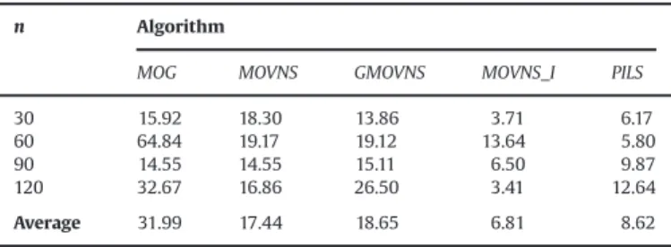
In Tables 3and 4 the results attained by the algorithms in relation to the distance metrics are presented. In Table 3 the results regarding the average distance and inTable 4the results regarding the maximum distance are presented.

Through Tables 3 and 4, it is veriﬁed that the MOVNS_I algorithm is the one that produces lower average values, that is, closer to zero, from the average and maximum distances to the majority set of instances. The MOVNS_I did not attain lower average values to the set of instances withn¼60 only wherePILS showed better results.

As presented inSection 6.2, the distance metrics measures the proximity between the solutions of a setDiand the solutions of set Ref. Therefore, the higher the percentage of solutions ofDiin the Refset, the lower tends to be the values of the distance metrics. The values of the distance metrics tend to be smaller, but those values also depend of the distance between Di solutions and solutions belonging toRefset obtained by other algorithms. For each group of 40 instances of size n, Table 5 shows average percentages of solutions obtained by the MOVNS_I and PILS algorithms which are part ofRefset.

Table 5shows that algorithms had presented very close values for the average percentage except for the set withn¼60. In this case, the percentage difference was 28.42%. For the groups of instances in which the difference between the average percen-tages was small, the MOVNS_I algorithm had presented better results forDavandDmax, even thePILSshowing higher percentage. However, when the difference between these average percentages was large, as in the case of the instances set withn¼60, better values for the distances was obtained by thePILS. Therefore, the MOVNS_I had presented in most cases a better performance regarding the distance metrics.

In Table 6 the values attained by the proposed algorithms regarding the hypervolume indicator are presented.

Through Table 6 it is veriﬁed that the GMOVNS algorithm presented lower average values, compared with the other algo-rithms, from the hypervolume indicator for all sets of instances.

InTable 7the results attained by the proposed algorithms are shown regarding theepsilonmetric.

ThroughTable 7it is veriﬁed that theGMOVNSis the algorithm that produces lower average values for theepsilon metric for all sets of instances.

In Table 8, the values attained by the algorithms proposed regarding the error ratio are presented.

As it can be observed inTable 8, thePILSalgorithms presented, in all sets of instances, a lower average value for the error ratio. This means that, based on error ratio, the algorithm PILS was superior to the others.

6.3.1. Analysis of the results

Based on the average values of the computational time spent by each algorithm to obtain the non-dominated solutions sets, we can see that all the algorithms were computationally efﬁcient, obtain-ing solutions sets in an acceptable time. For all the instances sets, Table 2

Average computational time.

n Algorithm

MOG MOVNS GMOVNS MOVNS_I PILS

30 0.18 0.42 0.39 1.05 1.12

60 1.01 3.93 3.01 4.12 10.98

90 2.78 13.21 11.04 15.79 53.44 120 7.69 54.13 36.40 57.70 143.34

Table 3

Distance metrics results–average distance (%).

n Algorithm

30 15.92 18.30 13.86 3.71 6.17

60 64.84 19.17 19.12 13.64 5.80

90 14.55 14.55 15.11 6.50 9.87

120 32.67 16.86 26.50 3.41 12.64

Average 31.99 17.44 18.65 6.81 8.62

Table 4

Distance metrics results–maximum distance (%).

n Algorithm

30 64.75 49.10 55.80 12.50 20.25 60 102.49 62.82 78.55 35.51 21.00 90 47.55 40.64 38.34 14.80 29.90 120 88.27 44.40 95.93 14.15 37.23

Average 75.76 49.24 67.15 19.24 27.01

Table 5

Average Percentages of Solutions of theMOVNS_IandPILSin theRefSet.

n Algorithm Difference

MOVNS_I PILS

30 56.70 59.80 3.10

60 27.10 55.52 28.42

90 36.67 38.63 1.96

120 42.12 44.22 2.10

Table 6

Hypervolume indicator results.

N Algorithm

30 925.78 616.44 352.12 373.22 367.21 60 1769.16 807.31 535.98 1433.66 888.32 90 2700.65 2351.28 1979.39 2143.45 2132.65 120 5165.89 5913.00 3715.94 3876.98 3800.99

(10)

the MOG and PILS algorithms had presented the lowest and highest average computational time, respectively.

Results attained from the computational experiments, showed that theGMOVNSalgorithm had best performance. TheGMOVNS has generated better results for two of the four multi-objective performance measures assessed: hypervolume indicator and epsi-lon metric. This means that the GMOVNSalgorithm produces a better coverage for the Pareto-optimal front and that the non-dominated solutions generated by this algorithm are closer to the Refset. Regarding the distance metrics, in general, theMOVNS_I algorithm has obtained the lowest average values for these metrics. Therefore, theMOVNS_I has achieved better distributed solutions throughout theRefset. For all the instances sets, thePILS algorithm had obtained the better results for the error ratio. The PILShad presented, on average, the higher percentage of solutions belonging to theRefset.

Table 9shows a comparison between the results obtained by the proposed algorithms and those obtained by Viana and Sousa

[12]. This comparison was made regarding the average values obtained for the distance metrics, for instances with 30 activities from PSPLib.

ThroughTable 9it is veriﬁed that all the proposed algorithms presented lowest computational effort compared with the pro-posed algorithms by Viana and Sousa[12]. Regarding the distance metrics, theMOVNS_IandPILShave obtained better results, that is, values closer to zero, compared to the PSA and MOTS proposed by Viana e Sousa[12]. Therefore, theMOVNS_IandPILShave achieved better distributed solutions throughout the Ref set. Only the MOVNS has obtained worst results for the two distances, com-pared with the MOTS.

Table 10presents a comparison between the results obtained by the proposed algorithms and those obtained by Ballestín and Blanco [6]. The comparison was performed using the average values obtained for the average distance metric, for instances with 120 activities from PSPLib. The used results were obtained by Ballestín and Blanco [6]limiting the number of generated solu-tions in 5000, the same way that in this work.

ThroughTable 10it is veriﬁed that, except theMOG, all the other proposed algorithms have obtained better results for the average distance, that is, values closer to zero, compared to the SPEA-II,

NSGA-II and PSA proposed by Ballestín and Blanco[6]. TheMOGhas obtained better results only compared to the PSA. Therefore, the MOVNS,GMOVNS,MOVNS_IandPILShave achieved better distributed solutions throughout theRefset.

To compare results, no work was found in literature using the hypervolume indicator, epsilon or error ratio to assess multi-objective algorithms applied to the RCPSPRP.

6.4. Statistical analysis

The experiments that follow aim at verifying, if there is a signiﬁcant difference between the algorithms proposed in this paper, concerning the multi-objective performance measures used. These experiments were conducted with the assistance of the Minitabs computational package on its 16th version. It is emphasized here that this experimentation enables the researchers to make inferences to the population of all instances.

To conduct the experiments, the statistical technique Analysis of Variance (ANOVA) was chosen, as described by Montgomery

[41]. The interest is then to test the equality of the population means (

μ

) to theﬁve implemented algorithms against the inequality of the means.

In the ANOVA application two hypotheses were tested:

H0:

μ

₁¼

μ

₂¼

μ

₃¼

μ

₄¼

μ

₅ ð10Þ

H1: μ

iaμj;for at least one pairði;jÞ;withi;j¼1;2;3;4;5 andiaj ð11Þ

In tests(10) and (11), the null hypothesis(10)represents the equality of the population means hypothesis in relation to the analyzed multi-objective performance measure on theﬁve algo-rithms, that is, it conjectures that there is no signiﬁcant difference between these algorithms regarding the metric. Hypothesis(11), on the other hand, conjectures the opposite.

However, to apply the ANOVA, the sample data should be normally distributed in this case, and the population variances (s2) approximately equal between the factor levels, regarding the algorithms proposed here.

Although the test is based on the supposition that the sample data should be normally distributed, according to Kulinskaya et al.[42], Table 7

Epsilonmetric results.

N Algorithm

30 1.47 1.93 1.21 1.82 1.25

60 1.44 1.75 1.28 1.50 1.44

90 1.88 1.85 1.58 1.91 1.80

120 1.36 1.70 1.21 1.90 1.50

Average 1.54 1.81 1.30 1.78 1.50

Table 8

Error ratio results (%).

n Algorithm

30 77.20 40.72 59.62 43.30 40.20 60 86.19 74.65 66.94 72.90 44.48 90 89.65 62.11 75.15 63.33 61.37 120 91.47 90.52 67.01 57.88 55.78

Average 86.13 67.00 67.18 59.35 50.46

Table 9

Comparison of average values forDav,Dmzxand computational time (in seconds).

Algorithm Dav Dmax Computational time

MOG 15.92 64.75 0.18

MOVNS 18.30 49.10 0.42

GMOVNS 13.86 55.80 0.39

MOVNS_I 3.71 12.50 1.05

PILS 6.17 20.25 1.12

PSA[12] 32.19 41.76 2590 MOTS[12] 16.63 33.86 2599

Table 10

Comparison of average values forDav.

Algorithm Dav

MOG 32.67

MOVNS 16.86

GMOVNS 26.50

MOVNS_I 3.41

PILS 12.64

SPEA-II[6] 27.00

NSGA-II[6] 27.00

(11)

this hypothesis is not critical when the sizes of the samples are at least 15 or 20. Once all the samples on this work have the equal size to 160 (number of instances used) for each algorithm, thus, the normality is not critical. Hence, the normality premise is veriﬁed for all the algorithms regarding all metrics. To use the ANOVA it is needed, then, the veriﬁcation of only the variances proximity between the data from the algorithms regarding each metrics. For this, the following hypotheses were tested:

H0: s2

1 ¼s2

2 ¼s2

3 ¼s2

4 ¼s2

5 ð12Þ

H1: s2_i as2_j for at least one pairði;jÞ;withi;j¼1;2;3;4;5 andiaj ð13Þ

In tests(12) and (13), the null hypothesis(12)represents the equality of the population variances hypothesis in relation to the analyzed multi-objective performance measure on theﬁve algo-rithms. Hypothesis(13)conjectures the opposite.

By applying these hypothesis tests is possible to calculate a test statistic that allows us to accept or reject the null hypothesis. In Statistical Inference is usual to represent this test statistic for p-value. From the value of this test statistic and of a criterion for acceptance/rejection is possible to conclude, with a signiﬁcance level

α

deﬁneda priori, which of the hypotheses accept. That is, if

α

Zp-value rejects H0. All the tests in this section have been executed with a signiﬁcance level

α

¼0.05 (5%).

Nevertheless, the ANOVA does not tell us which pairs of algorithms present signiﬁcant differences, that is, result in differ-ent means to each assessed metric. To answer this question the method of the Least Signiﬁcant Difference (LSD), also known as Fisher's method[41], is used.

All the tables of ANOVA results presented in this section show the calculated value of thep-value, the sample means, the sample standard deviations and the interval limits with 95% of conﬁdence on the population means from the analyzed multi-objective performance measure, in accordance with each algorithm.

Distance Metrics

For the distance metrics the hypothesis tests (12) and (13) were used to verify the proximity of variances between the data of all algorithms. Thep-valuestatistics calculated for this test was equal to 0.075 for the average distance, and 0.055 for the maximum distance. Once

α

op-value for both distance metrics, the variance equality hypothesis is accepted between the population data to theﬁve algorithms. Therefore, once the premise is veriﬁed, the ANOVA is applied to the concerning data from the metrics.

The application of ANOVA to the average distance data allowed us to calculate the values presented inTable 11. According to the results inTable 11,p-value¼0.027. Therefore, it can be stated that the null hypothesis should be rejected, that is, as

α

Zp-value, there are enough statistical evidences

to conclude that the average values regarding the average distance are different on each algorithm. By using the LSD method, it can be stated that there are statistical evidences showing that the average values, regarding the average

distance, are different within the following algorithm pairs: MOGMOVNS_IandMOGPILS.

The application of ANOVA to the maximum distance data allowed us to calculate the values presented inTable 12. According to the results inTable 12, p-value¼0.004. There-fore, it can be stated that the null hypothesis should be rejected, that is, as

α

Zp-value, there are enough statistical

evidences to conclude that the average values regarding the maximum distance are different on each algorithm. By using the LSD method, it can be stated that there are statistical evidences showing that the average values regarding the max-imum distance, are different within the following algorithm pairs:MOGMOVNS,MOGMOVNS_IandMOGPILS.

Hypervolume Indicator

For the hypervolume indicator it was veriﬁed the proximity of variances between the data of all algorithms by the hypoth-esis tests(12) and (13). The calculatedp-valuestatistics was equal to 0.560 and, as

α

o_p-value_{, the hypothesis of the}

variances equality between the population data on theﬁve algorithms is accepted. Once veriﬁed the premise, the ANOVA is applied to the data of this metric.

The application of ANOVA to the hypervolume indicator data allowed us to calculate the values presented inTable 13. According to the results inTable 13, p-value¼0.443. There-fore, it can be stated that the null hypothesis should be accepted, that is, as

α

op-value, there are enough statistical evidences to conclude, with a 5% signiﬁcance level (

α

¼0.05), that the average values regarding the hypervolume indicator equal within all algorithms.

Epsilon metric

For the epsilon metric it was veriﬁed the proximity of variances between the data of all algorithms by the hypoth-esis tests(12) and (13). The calculatedp-valuestatistics was equal to 0.077 and, as

α

o_p-value_{, the hypothesis of the}

variances equality between the population data on theﬁve algorithms is accepted. Once veriﬁed the premise, the ANOVA is applied to the data of this metric.

The application of ANOVA to theepsilonmetric data allowed us to calculate the values presented inTable 14.

According to the results inTable 14,p-value¼0.026. Therefore, it can be stated that the null hypothesis should be rejected, that is, as

α

Zp-value, there are enough statistical evidences

to conclude that the average values regarding the epsilon metric are different between the algorithms. By using the LSD method, it can be stated that there are statistical evidences showing that the average values, regarding theepsilonmetric, are different within the following algorithm pairs:GMOVNS MOVNSandGMOVNSMOVNS_I.

Error ratio

For the error ratio the hypothesis tests(12) and (13) were used to verify the proximity of variances between the data of all algorithms. The calculatedp-valuestatistics was equal to 0.008 and, as

α

4p-value, the hypothesis of the variances equality between the population data on theﬁve algorithms is rejected. Therefore, this premise is not veriﬁed, and consequently, the

Table 11

The results of ANOVA for the average distance.

p-Value, 0.027

Algorithm

Mean 32.0 17.4 18.6 6.8 8.6

Standard deviation 102.8 29.3 31.5 10.5 10.8

(12)

ANOVA cannot be applied to this metric's data. As a result, the Kruskal-Wallis non-parametric test [43] was used. The differ-ence from ANOVA to the Kruskal-Wallis non-parametric test is that the later, instead of working with means, uses population medians (

η

). The test can be used to verify the medians equality of two or more populations and, applying to this work, tests the following hypothesis:

H0:

η

₁ ¼

η

₂ ¼

η

₃ ¼

η

₄ ¼

η

₅ ð14Þ

H1:

η

_i a

η

jfor at least one pairði;jÞ; withi;

j¼1;2;3;4;5 andiaj ð15Þ

In tests(14) and (15), the null hypothesis(14)represents the equality of the population medians hypothesis in relation to the error ratio on the ﬁve algorithms, that is, it conjectures that there is no signiﬁcant difference between these algorithms regarding this metric. Hypothesis (15), on the other hand, conjectures the opposite.

For this test of hypothesis, the p-value statistics calculation brought the value 0.001. Once the signiﬁcance level

α

¼0.05 is adopted and

α

4p-value, the median equality between the population data on the ﬁve algorithms should be rejected. Hence, it is statistically concluded that the algorithms differ in error ratio. By comparing the pairs of algorithms, it can be stated that there are statistical evidences that the median values from the error ratio are different between: MOGMOVNS, MOGGMOVNS, MOGMOVNS_I, MOGPILS, MOVNSPILS andGMOVNSPILS.

7. Conclusions

This work addressed the resource-constrained project schedul-ing problem with precedence relations as a multi-objective opti-mization problem, having two optiopti-mization criteria that were

tackled: the makespan minimization and the minimization of the total weighted start time of the activities.

To solve the problem,ﬁve algorithms were implemented:MOG, MOVNS,MOGusing VNSas local search, denominated GMOVNS; MOVNSwith intensiﬁcation procedure based on Ottoni et al.[24], denominatedMOVNS_I; andPILS.

The algorithms were tested in 160 instances adapted from literature, and compared using four multi-objective performance measures: distance, hypervolume,epsilonand error ratio. Based on the results attained from the computational experiments, we can see that all algorithms were computationally efficient, obtaining sets of non-dominated solutions in an acceptable time, and three conclusions were obtained: first, the MOVNS_I has shown to be superior than the other algorithms on the majority of instances, regarding the distance metrics; second, the GMOVNSis superior regarding the hypervolume indicator and theepsilonmetric; and third, the algorithm PILS is superior regarding the error ratio. Statistical experiments were conducted and have revealed that there is a significant difference between some proposed algo-rithms concerning the distance, epsilon, and error ratio metrics. However, significant difference between the proposed algorithms with respect to hypervolume indicator was not observed.

Acknowledgments

The authors would like to thank the UFOP, UFV and FAPEMIG for their support and incentive in the development of this work.

References

[1]Oguz O, Bala H. A comparative study of computational procedures for the resource constrained project scheduling problem. Eur J Oper Res 1994;72:406–16.

[2]Garey MR, Jonhson DS. Computers and intractability: a guide to the theory of NP-completeness. New York: W.H. Freeman and Company; 1979.

Table 12

The results of ANOVA for the maximum distance.

p-Value, 0.004

Algorithm

Mean 75.8 49.2 67.1 19.2 27.0

IC (μ, 95%) (19.9; 143.1) (29.8; 68.1) (24.9; 106.6) (12.5; 25.6) (18.0; 35.9)

Table 13

The results of ANOVA for the hypervolume indicator.

p-Value, 0.443

Algorithm

Mean 2640.4 2422.0 1645.9 1956.8 1797.3

IC (μ, 95%) (1645.3; 3654.9) (1290.7; 3296.3) (934.3; 2416.2) (1105.3; 2812.2) (865.2; 2694.1)

Table 14

The results of ANOVA for theEpsilonmetric.

p-Value, 0.026

Algorithm

Mean 1.54 1.81 1.30 1.78 1.50

(13)

[3]Thomas PR, Salhi S. A Tabu search approach for the resource constrained project scheduling problem. J Heuristics 1998;4:123–39.

[4]Slowinski R. Multi-objective project scheduling under multiple-category resource constraints. Advances in project scheduling. Amsterdam: Elsevier; 1989.

[5]Martínez-Irano M, Herrero JM, Sanchis J, Blasco X, Garcia-Nieto S. Applied Pareto multi-objective optimization by stochastic solvers. Eng Appl Artif Intell 2009;22:455–65.

[6]Ballestín F, Blanco R. Theoretical and practical fundamentals for multi-objective optimization in resource-constrained project scheduling problems. Comput Oper Res 2011;38:51–62.

[7]Jones DF, Mirrazavi SK, Tamiz M. Multi-objective metaheuristics: an overview of the current state-of-art. Eur J Oper Res 2002;137:1–19.

[8] Hansen MP. Tabu search for multi-objective optimization: MOTS. In: Proceed-ings of the 13th international conference on multiple criteria decision making. University of Cape Town; 1997. p. 6–10.

[9]Czyzak P, Jaszkiewicz A. Pareto simulated annealing – a metaheuristic technique for multiple-objective combinatorial optimization. J Multi-Criteria Decis Anal 1998;7:34–47.

[10]Deb K, Agrawal S, Pratap A, Meyarivan T. A fast elitist nondominated sorting genetic algorithm for multi-objective optimization: NSGA-II. In: Schoenauer M, editor. Parallel problem solving from nature (PPSN VI). Berlin, Germany: Springer; 2000. p. 849–58.

[11]Zitzler E, Laumanns M, Thiele L. SPEA2: improving the strength Pareto evolutionary algorithm. Zurich, Switzerland: Computer Engineering and Net-works Laboratory (TIK); 2001.

[12]Viana A, Sousa JP. Using metaheuristics in multi-objective resource con-strained project scheduling. Eur J Oper Res 2000;120:359–74.

[13] Kazemi FS, Tavakkoli-Moghaddan R. Solving a multi-objective multi-mode resource-constrained project scheduling with discounted cash ﬂows. In: Proceedings of the 6th international management conference. Tehran, Iran; 2008.

[14]Abbasi B, Shadrokh S, Arkat J. Bi-objective resource-constrained project scheduling with robustness and makespan criteria. Appl Math Comput 2006;180:146–52.

[15]Al-Fawzan MA, Haouari M. A bi-objective model for robust resource-constrained project scheduling. Int J Prod Econ 2005;96:175–87.

[16]Aboutalebi RS, Najaﬁ AA, Ghorashi B. Solving multi-mode resource-con-strained project scheduling problem using two multi-objective evolutionary algorithms. Afr J Bus Manage 2012;6(11):4057–65.

[17] Reynolds AP, Iglesia B. A multi-objective GRASP for partial classiﬁcation. Soft Comput 2009;13:227–43.

[18] Geiger MJ. Randomized variable neighborhood search for multi-objective optimization. 4th EU/ME: design and evaluation of advanced hybrid meta-heuristics; 2008. p. 34–42.

[19] Geiger MJ. Foundations of the Pareto iterated local search metaheuristic. In: Proceedings of the 18th MCDM. Chania, Greece; June 2006.

[20]Arroyo JEC, Vieira PS, Vianna DS. A GRASP algorithm for the multi-criteria minimum spanning tree problem. Ann Oper Res 2008;159(1):125–33. [21]Minella G, Ruiz R, Ciavotta MA. Review and evaluation of multi-objective

algorithms for the ﬂowshop scheduling problem. INFORMS J Comput 2010;20:451.

[22] Oliveira Junior PL, Arroyo JEC, Souza VAA. Heurísticas GRASP e ILS para o Problema No-wait Flowshop Scheduling Multiobjetivo. In: Proceedings of the

17th Simpósio Brasileiro de Pesquisa Operacional. Bento Gonçalves, Brasil; 2010.

[23]Arroyo JEC, Ottoni RS, Oliveira AP. Multi-objective variable neighborhood search algorithms for a single machine scheduling problem with distinct due windows. Electron Notes Theor Comput Sci 2011;281:5–19.

[24] Ottoni RS, Arroyo JEC, Santos AG, Algoritmo VNS. Multiobjetivo para um Problema de Programação de Tarefas em uma Máquina com Janelas de Entrega. In: Proceedings of the 18th Simpósio Brasileiro de Pesquisa Oper-acional. Ubatuba, Brasil; 2011.

[25]Koné O, Artigues C, Lopez P, Mongeau M. Event-based MILP models for resource-constrained project scheduling problems. Comput Oper Res 2009;38:3–13.

[26]Kolisch R. Serial and parallel resource-constrained project scheduling meth-ods revisited: theory and computation. Eur J Oper Res 1996;90:320–33. [27]Kelley JE. The critical method: resources planning and scheduling. Industrial

scheduling. New Jersey: Prentice-Hall; 1963; 347–65.

[28]Feo TA, Resende MGC. Greedy randomized adaptive search procedures. J Glob Optim 1995;40:109–33.

[29]Mladenovic N, Hansen P. Variable neighborhood search. Comput Oper Res 1997;24:1097–100.

[30]Lourenço HR, Martin OC, Stüzle T. Iterated local search. In: Glover F, Kochenberger GA, editors. Handbook of metaheuristics. Dordrecht, Nether-lands: Kluwer Academic; 2003. p. 320–53.

[31]Deiranlou M, Jolai FA. New efﬁcient genetic algorithm for project scheduling under resource constraint. World Appl Sci J 2009;7:987–97.

[32]Agarwal A, Colak S, Erenguc SA. Neurogenetic approach for the resource-constrained project scheduling problem. Comput Oper Res 2011;38:44–50. [33]Kolisch R, Sprecher A. PSPLib–a project scheduling problem library. Eur J

Oper Res 1996;96:205–16.

[34] PSPLib.〈http:/129.187.106.231/psplib/〉.

[35]Hansen M, Jaszkieweiz A. Evaluating the quality of approximations to the non-dominated set. Department of Mathematical Modeling, Technical University of Denmark; 1998 ([technical report]).

[36]Veldhuizen D. Multi-objective evolutionary algorithms: classiﬁcations, ana-lyses and new innovations. Dayton, Ohio: School of Engineering of the Air Force Institute of Technology; 1999 ([Ph.D. thesis]).

[37]Zitzler E, Ded K, Thiele L. Comparison of multi-objective evolutionary algo-rithms: empirical results. Evol Comput 2000;8:173–95.

[38]Deb K, Jain S. Running performance metrics for evolutionary multi-objective algorithms. Kanpur Genetic Algorithms Laboratory, Indian Institute of Tech-nology Kanpur, India; 2002 ([technical report]).

[39] Fonseca C, Knowles J, Thiele L, Zitzler EA. Tutorial on the performance assessment of stochastic multi-objective optimizers. In: Proceedings of the 3th international conference on evolutionary multi-criterion optimization (EMO). Guanajuato, Mexico; 2005.

[40]Coello CA, Lamont GB. Applications of multi-objective evolutionary algo-rithms. world scientiﬁc printers. Singapore: Pte Ltd.; 2004.

[41]Montgomery DC. Design and analysis of experiments. 7th ed.. New York: John Wiley and Sons; 2009.

[42]Kulinskaya E, Staudte RG, Gao A. Power approximations in testing for unequal means in a one-way ANOVA weighted for unequal variances. Commun Stat 2003;32(12):2353–71.