This work aims to investigate the viability and convenience of adopting a variable limit a1 for the instability parameter of buildings with reinforced concrete wall-frame or core-frame structures. Initially, the evolution of tall buildings global stability theory is summarized, giving emphasis to deine when a second order analysis is needed. The treatment given to this subject by the present Brazilian code for concrete structures design (NBR 6118:2007) is also showed. It follows a detailed analytical study that led to the derivation of an equation for the variable limit a1; a series of examples is presented to check its accuracy. Results are analyzed, showing the validity bounds of the equation and research directions are sug -gested, in order to improve it.
Keywords: instability, bracing structures, second order.
O presente trabalho tem por objetivo investigar a viabilidade e a conveniência de se adotar um limite variável a1 para o parâmetro de instabilidade de edifícios com estruturas de concreto armado, constituídas por associações de pórticos com paredes ou núcleos. Inicialmente, é feito um re-sumo da evolução da teoria sobre a análise da estabilidade global de edifícios altos, especialmente sobre a deinição da necessidade ou não de se realizar uma análise de segunda ordem; mostra-se também como esta questão é tratada pela atual norma de projeto de estruturas de concreto (NBR 6118:2007). Na seqüência, apresenta-se um detalhado estudo analítico que levou ao estabelecimento de uma fórmula para o limite variável a1, seguido de uma série de exemplos para testar a validade da mesma. Os resultados são analisados, mostrando-se os limites de validade da fórmula e indicando-se linhas de investigação no sentido de aperfeiçoá-la.
Palavras-chave: instabilidade, estruturas de contraventamento, segunda ordem.
A variable limit for the instability parameter of
wall-frame or core-frame bracing structures
Um limite variável para o parâmetro de instabilidade
de estruturas de contraventamento formadas por
associações de pórticos com paredes ou núcleos
R. J. ELLWANGER a [email protected]
a Professor Associado, Departamento de Engenharia Civil, Universidade Federal do Rio Grande do Sul, e-mail: [email protected],
endereço postal: Rua Marcelo Gama 1189/401, CEP 90540-041, Porto Alegre-RS, Brasil.
Received: 14 Sep 2011 • Accepted: 18 Nov 2011 • Available Online: 01 Feb 2012
Abstract
1. Introduction
1.1 Second order effects in building structures
Depending on its lexibleness, a building bracing structure, when simultaneously subject to gravity and wind loads, may develop addi -tional effects to those usually obtained in a irst order linear analysis (in which the equilibrium is veriied in the non deformed structure). They are the second order effects, in whose computation the mate-rial nonlinear behavior (physical nonlinearity) and the structure de -lected shape (geometric nonlinearity) must be considered. The work of Beck and König [1], brought in 1967, represented an im -portant advance in the development of tall buildings global stability analysis. A very easy criterion to apply was established, determining that the second order effects may be neglected, provided that they don’t represent an increase more than 10% on the irst order effects. Figure 1 shows the simpliied model for the bracing system. At irst, all bracing substructures are grouped in a single column, while all braced elements (bearing elements that don’t belong to the bracing system) are replaced by an assemblage of hinged bars, as shown in igure 1-a. The wind is considered by means of a w rate uniform load. P and V are the loor vertical loads, applied on the bracing sub -structures and braced elements, respectively. The loads w, P and V are considered with their characteristic values. Thereafter, in order to make possible to determine the second order effects by means of a continuum analysis, an equivalent approximate model, shown in igure 1-b, is adopted, with a continuous and uniform distribution of loors and vertical loads (p = P/h e v = V/h).
Concerning to the inluence of the loads V, acting on the braced elements, Beck and König [1] proved that, when the system dis -torts laterally, horizontal forces are transmitted through the loor
members to the bracing system, increasing the bending moment on its support. It can be proved that this increase is given by the sum of the forces V multiplied by the horizontal displacements of the respective loors. Therefore, in order to compute this bending moment including second order effects, the vertical loads acting on the bracing system would be given by the sum of its proper P loads and V loads.
In 1978, the criterion proposed by Beck and König [1] was included in the Comité Euro-International du Béton recommendations (CEB [2]). Its application consists in comparing the global bending mo -ments at the bracing system support M I (considering only irst or -der effects) and M II (including second order effects):
(1)
I
II
M
M
£
,1
1
or
(2)
2
75
1
1
1
8
75
1
1
1
2
75
1
23 2
tot
tot
tot
,
,
wH
EJ
v)H
(p
,
wH
,
£
´
+
-×
It can be noted that M Iand MII are due to factored loads, since the rates w, p and v are multiplied by 1,75. On the other hand, the physical nonlinearity is regarded taking EJ = 0,7 EcmJ for the structural members, where EcmJ represents the sum of the bracing substructures stiffness coeficients at the non cracked stage. Thus, performing this substitution leads to the condition:
Figure 1 – Simplified model for the bracing system
[2], on determining in its section 15 that the second order global effects are negligible when lower than 10% of the respective irst order effects (ixed nodes structure). In order to “verify the possibil -ity of dispensing the consideration of second order global efforts, in other words, to deine if the structure may be classiied as a ixed nodes one, without the need of a rigorous analysis”, ABNT [8] presents two approximate procedures, based respectively on the instability parameter and the gz factor. The irst one just consists of the Beck and König [1] criterion application and determines that: “A symmetrical framed structure may be considered as a ixed nodes one, if its instability parameter a will be lesser than the a1 value, according to the expressions:
(5)
)
/(
CS Ck
tot
N
E
I
H
=
a
(6)
4
6
,
0
3
1,
0
2
,
0
11
=
+
n
'
n
£
Ù
a
=
'
n
³
a
“n is the number of horizontal bars levels (loors) above the founda -tion or a slightly displaceable subsoil level. Htot is the structure total height, measured from the foundation top or a slightly displaceable subsoil level. Nk is the summation of all vertical loads acting on the structure (from the level considered for Htot computation), with their characteristic values. ECSIC represents the summation of all column stiffness values in the considered direction. In the case of framed, trussed or mixed structures, or columns with variable stiffness along the height, the ECSIC value of an equivalent column with constant section may be considered”. The determination of this equivalence will be seen in section 2.1. IC is the moment of inertia considering columns gross sections. ECS is the secant elas-ticity modulus, expressed by:
(7)
2/ 1
5600
85
,
0
85
,
0
Ci ckCS
E
f
E
=
=
´
ECS, ECi (tangent elasticity modulus) and fck (compressive charac-teristic strength) are given in MPa. The NBR 6118 code also ad -opted the Franco [5] propositions on determining different a1 val-ues, depending on the bracing structure type: “The limit value a1 = 0,6, prescribed for n > 4, is generally applicable to the building usual structures. It may be adopted for wall-columns assemblages and rigid frames associated to wall-columns. It may be increased until a1 = 0,7 in the case of bracing systems composed exclusively by wall-columns and must be reduced to a1 = 0,5 if there are only rigid frames.”
In a second order analysis, the effects of both physical and geomet-ric nonlinearities must be considered. ABNT [8], in its item 15.7.3, allows that the physical nonlinearity can be considered in an ap-proximated manner, on calculating second order global efforts in framed structures with four or more loors. This is done by means of a reduction of the structural members (EI)sec stiffness factors as
(3)
0,54
)
/(
)
(
tot cmtot
p
+
v
H
E
J
£
H
According to Vasconcelos [3], the results obtained by Beck and König [1] could be applied only to building structures whose lat -eral stiffness was concentrated in few columns rigidly connected among themselves, in order to be considered as a single column. The correspondence of this model with other types of bracing sys-tems (variable section walls, rigid frames etc.) came to be done through the equality of horizontal displacements due to horizontal loads. The equivalent column would be that one with a stiffness factor EJ such that the resulting horizontal displacements were the same of the structure under consideration, for the same hori-zontal loading. With the purpose of simpliication, this equivalent stiffness came to be determined based on the actuation of a unit horizontal load at the building top. In Brazil, the procedure came to be applied changing the load factor from 1,75 to 1,40 – see, for example, Sussekind [4] – and came to be known as minimal stiff -ness check. Consequently, inequality (3) changed to:
(4)
0,60
)
/(
)
(
tot S 28 Itot
p
+
v
H
E
-J
£
H
where ES-28 is the concrete secant elasticity modulus at 28 days and JI is the sum of bracing substructures inertias at non cracked stage. In 1985, Franco [5] proposed that the equivalent column stiff -ness have to be obtained based on the actuation of a uniformly dis-tributed horizontal load, in place of the top unit load. Furthermore, he preconized that the delected shape of the bracing structure can affect the Beck and König [1] criterion application. Thus, the coef -icient on the inequality (4) right hand would have its value deined as a function of the bracing type:
- walls or cores: coeficient 0,7;
- wall-frame or core-frame structures: coeficient 0,6; - only rigid frames: coeficient 0,5.
In 1995, Franco [6], dealing with the physical nonlinearity consid -eration through structural members stiffness reduction, proposed different reduction factors, speciic for slabs, column members and beam members with symmetrical and asymmetrical reinforcement. Although not belonging to this work purpose, a mention deserves to be made to the method based on the moment ampliication fac -tor gz, presented in 1991 by Franco and Vasconcelos [7]. It also ap -plies the criterion of 10% increase in relation to irst order effects, to deine if a second order analysis is or not needed; however, in this case it is done for each combination of horizontal and verti-cal loads. Furthermore, under certain conditions, this method may itself constitute a second order analysis. These features caused this method to be rapidly disseminated and largely employed in buildings structures design.
1.2 ABNT NBR 6118 prescriptions
nance of frames, when a value lesser than 0,6, possibly close to 0,5, should be adopted.
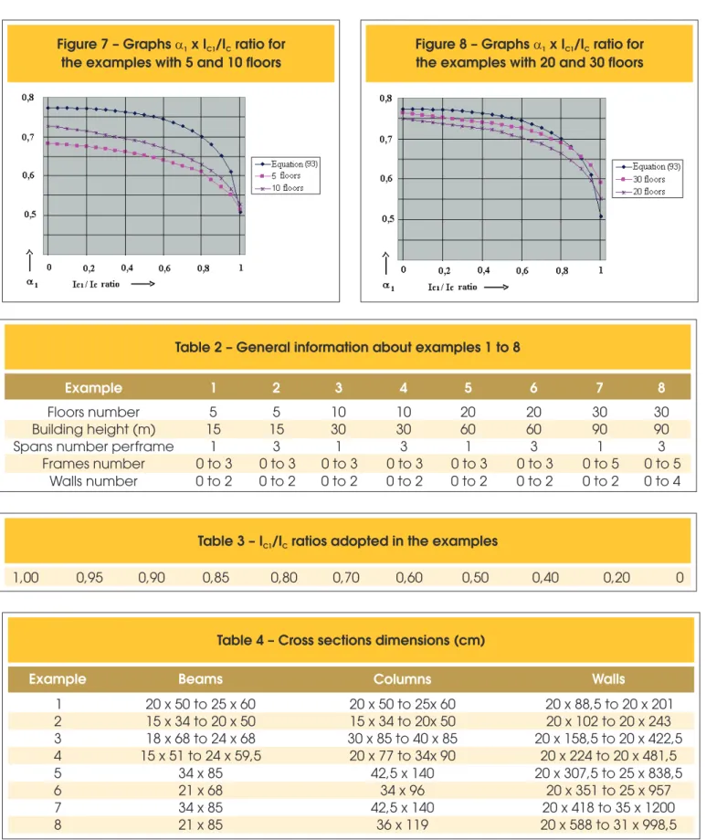
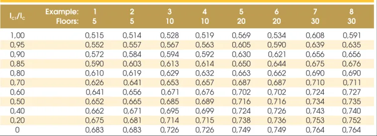
These errors, if expressed in relation to a1, are apparently small. However, is must be remembered that the instability parameter computation requires a square root extraction. Consequently, on verifying the exemption of performing a second order analysis, the error on determining the needed stiffness can become signiicant. This work aims to research a way of deining the instability parameter limit a1 for associations of rigid frames and walls/cores, variable with their stiffness factors proportion. At irst, the linear behavior formula -tion for these associa-tions is presented, followed by an analytical study about the geometric nonlinear behavior of isolated walls/cores and rigid frames and then of their association. This study is based on the simpli-ied model presented in section 1.1, applying the criterion expressed by inequality (1); the differential equations are solved by Galerkin method. Right away, the formula found for the variable limit a1 is tested in a series of examples of buildings braced by wall-frame associations. 88 tests are performed, varying the number of loors, of frame spans and the proportion between the stiffness factors of frames and walls.
2. Linear analysis
2.1 Equivalence between bracing substructures
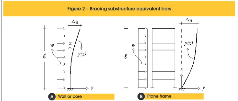
The substructures of the wall or core types distinguish themselves by a high stiffness to shear, predominating lexural delections. They may be modeled by simple beams, ixed on the building sup -port, behaving as columns. Figure 2-a shows a wall or core, mod -eled by a cantilever bar of length l, subject to an uniformly distribut
-ed horizontal load of ratio w. Representing the material longitudinal elasticity modulus, the constant section moment of inertia and the bending moment function respectively by E, J and M(x), the differ-ential equation of motion may be expressed as:
(13)
2
/
)
(
)
(
/
/
2 22
y
dx
E
J
d
dx
M
x
w
x
d
J
E
=
f
=
=
l
-Bending moments inducing tension on the bar left side are posi -tive, the delected concavity becoming turned to right (f(x) is its slope). Introducing the appropriate boundary conditions, y(x) and the top horizontal displacement DH are obtained:
(14)
ú
ú
û
ù
ê
ê
ë
é
-+
÷
ø
ö
ç
è
æ
-=
1
4
1
24
)
(
4 4l
l
x
x
EJ
w
x
y
l
(15)
EJ
w
y
H
=
(
l
)
=
l
4/
8
D
In substructures of the rigid frame type, the delections due to bend -ing of the individual beam and column members are predominant. When the frame is subject to horizontal loads, the global bending moment is mainly carried to the columns as axial efforts, for which a function of ECiIC, or of ECSIC if equation (7) is used. Representing
by As and As’, respectively, the tensile and compressive longitudi-nal reinforcements areas, the following expressions can be written: - slabs:
(8)
CCS C
Ci
I
E
I
E
EI
)
0
,
3
0
,
353
(
sec=
=
- beams:
(9)
'sec
0
,
4
0
,
471
)
(
EI
=
E
CiI
C=
E
CSI
C'
A
s¹
A
s(10)
' sec0
,
5
0
,
588
)
(
EI
=
E
CiI
C=
E
CSI
C'
A
s=
A
s- columns:
(11)
C CS C
Ci
I
E
I
E
EI
)
0
,
8
0
,
941
(
sec=
=
Furthermore, when the bracing substructure is exclusively con-stituted by beams and columns (rigid frame) and the “importance factor” of the second order global efforts (gz) is lesser than 1,3 (cor -responding to a “bland” nonlinearity) it is allowed to consider the stiffness of the rigid frame members as a whole, as follows:
(12)
CCS C
Ci
I
E
I
E
EI
)
0
,
7
0
,
824
(
sec=
=
1.3 Reasons and targets of the research
The ABNT [8] code represented an improvement in relation to the preceding one, on establishing procedures for checking if second order global effects are unnecessary to consider. Con -cerning to the instability parameter for buildings with four or more loors, it treated differently the various types of bracing systems, on determining different values for the a1 limit. How-ever, the prescription of a ixed limit (a1 = 0,6) for associations of walls and/or cores with rigid frames is questionable. As the relation between the stiffness factors of walls/cores and frames can vary, a1 also can vary from 0,5 to 0,7. This can lead to two types of errors:
n on behalf of safety: in associations with predominance of walls/
cores, the code restricts a1 to 0,6, when a larger value, possibly close to 0,7, could be adopted;
-the structure has a high stiffness. The horizontal delections are mostly caused by global shear. Therefore, the rigid frames may be modeled as vertical bars extremely stiff to global bending, prevail-ing shear distortions.
Figure 2-b shows a rigid plane frame subject to an uniformly dis -tributed horizontal load of ratio w. It is modeled by a vertical bar predominantly deformable by shear. As shown in the igure, the delected shape of this bar characterizes itself by a maximum f(x) slope at basis and tending to zero at top, just the contrary that hap -pens to the bar simulating the wall or core. This slope is related with the differences between horizontal displacements at adjacent loors. In their turn, these differences are proportional to the global shear Q(x). According to Stamato [9], the delected shape for this case is described by the following equation:
(16)
)
(
)
(
)
(
/
dx
S
x
Q
x
w
x
dy
S
=
f
=
=
l
-The proportionality factor S represents the system (plane frame) stiff -ness to global shear; it corresponds to the G A / c factor of a bar with shear deformation, where G, A and c are, respectively, the shear modulus, the section area and the section shape factor. Solving equa -tion (16), y(x) is obtained, leading to the top horizontal displacement:
(17)
S
w
y
H
=
(
l
)
=
l
2/
2
D
The relations established in this section have as their purpose to obtain the inertia of a bar equivalent to a given rigid plane frame. The item 15.5.2 of ABNT [8] code, on dealing with the instability parameter, establishes a methodology to determine the ECSIC fac-tor of a constant section column, equivalent to a given rigid plane frame. According to this methodology, the above-mentioned stiff
-ness factor should be obtained computing initially the horizontal displacement on the bracing structure (frame) top, under the hori -zontal loading, which is just DH given by (17). The next step is to obtain the stiffness of an equivalent column with constant section such that, under the same loading, undergoes the same top hori-zontal displacement which, in this case, is DH given by (15). This implies in equality between the two expressions for DH, resulting:
(18)
2/
4
E
J
l
S
=
2.2 Association of rigid frames with walls and/or cores
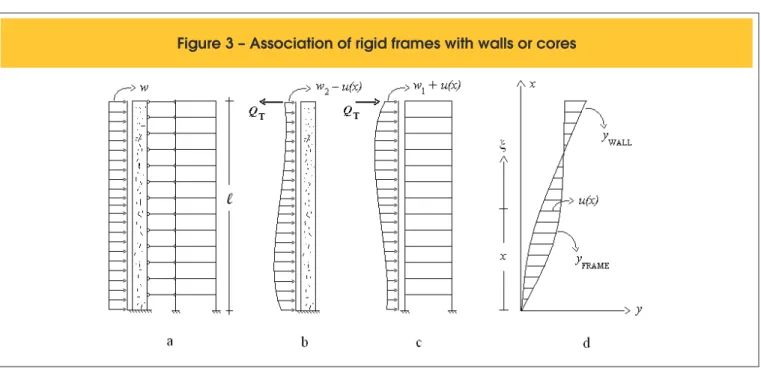
This section presents the formulation of the linear response of frame-wall/core structures, in order to that it have further on to be used by Galerkin method in obtaining an approximate solution for the nonlinear behavior of these structures. Figure 3-a shows the simpliied model of a bracing system composed by substruc -tures of the frame and wall/core types. The model consists in a wall (representing all system walls and cores) and a rigid frame (representing all system frames) connected among themselves by hinges (representing the loor slabs). An uniform distribution of rate w is admitted for the wind loads. EJ1 represents the stiffness of the frames set, according to equation (18). EJ2 represents the stiffness of the walls/cores set.
Figures 3-b and 3-c show the loads to that the wall and the frame will respectively be subject. These loads consist in top concen -trated forces (QT for the frame and –QT for the wall) and distributed forces that can be decomposed in constant and variable (along the height) parcels. The constant parcels (w1 for the frame and w2 for the wall) are such that w1 + w2 = w. The variable parcels (rate (u(x) for the frame and –u(x) for the wall), jointly with the forces QT, represent internal forces originated from the wall-frame interaction; since they are connected by the hinges, the wall and the frame
Figure 2 – Bracing substructure equivalent bars
Wall or core
BB
Plane frameare impeded to develop their natural delected shapes, as shown in igure 3-d. The frame will be subject to a global shear forces distribution given by:
(19)
ò
+
+
-=
l
lx
T
u
d
Q
x
w
x
Q
(
)
1(
)
(
x
)
x
As was seen in section 2.1, the frame behavior is described by equation (16). Writing this equation, introducing (18) and (19) and isolating the terms regarding to the internal forces, gives:
(20)
)
(
)
(
4
)
(
d
EJ
21x
w
1x
u
Q
x
T
+
ò
=
l
-
l
-l
f
x
x
In its turn, the wall will be subject to a bending moments distribu -tion given by:
(21)
ò
-=
l
l
lx
T
x
u
x
d
Q
x
w
x
M
(
)
(
)
2/
2
(
)
(
x
()
x
)
x
2
As was also seen in section 2.1, the wall behavior is described by equation (13). Writing this equation, introducing M(x) given by (21) and deriving both members, gives successively:
(22)
ò
-=
l
l
lx
T
x
u
x
d
Q
x
w
dx
d
EJ
f
(
)
2/
2
(
)
(
x
()
x
)
x
22
(23)
ò
+
+
-=
l
lx
T
u
d
Q
x
w
dx
d
EJ
f
2 2(
)
(
x
)
x
2 2
Substituting (20) into (23) and re-arranging:
(24)
0
)
(
)
(
)
(
4
2 1
21 2 2
2
d
dx
-
EJ
x
+
w
-
x
+
w
-
x
=
EJ
l
l
l
f
f
Considering that w1 + w2 = w (total wind load acting on the system) and deining a new variable K =
J
1/
J
2 , the solution for equa -tion (24) may be expressed as follows:(25)
)
(
4
)
(
1 2 /
2 2 / 2
1
e
C
e
w
EJ
x
C
x
=
Kx l+
- Kx l+
l
l
-f
where
(26)
1
e
2
e
8
42
1 3
1
=
K-
+
K
K
K
EJ
w
C
l
(27)
1
e
e
e
2
8
42 4
1 3
2
=
-
K+
+
K K
K
K
EJ
w
C
l
3. The Galerkin method
In many engineering problems, as the ones that are presented in the next sections, there arises the need to solve an equation of the type L(y) = 0, where L is a differential operator, whose solu-tion satisies to homogeneous boundary condisolu-tions. The Galerkin method consists in obtaining an approximate solution of the form:
(28)
å
=
=
n ix
a
x
y
1 i i
)
(
)
(
j
where
ϕ
i(
x
)
(i = 1, 2,..., n) are functions, previously chosen and satisfying to the same boundary conditions; the ai are coef-icients to be determined. The n functionsϕ
i(
x
)
must be linearly independent and belong to a system, represented by {ϕ
i(
x
)
} (i = 1, 2,..., n) and endowed of the completeness property in the solution domain. In order toy
(
x
)
be the exact solution of the given equation, it is necessary that L(y
) be identically null. This requirement, if L(y
) is considered to be continuous, is equiva -lent to the requirement of the orthogonality of the expression L(y
) to all the functionsϕ
i(
x
)
(i = 1, 2,..., n). However, having at disposal only n constants ai, only n orthogonality conditions can be satisied. Applying these conditions, the following system of equations is obtained:(29)
ò å
ò
×÷÷
=
=
ø
ö
ç
ç
è
æ
=
×
= D
n
j
n
i
dx
x
x
a
L
dx
x
x
y
L
(
(
))
(
)
(
)
i(
)
0
(
,1
,2
..
,.
)
1 j j
D
j
ij
j
The solution of this system (a linear one, in the case of a linear operator L) provides the values of the coeficients ai, from which the approximate solution
y
(
x
)
is obtained. The proof of conver-gence, as well as more detailed considerations about the Galerkin method can be seen in Kantorovich and Krylov [10].4. Exemption of the second order effects
consideration
The sections 4.1 and 4.2 present the formulation of the geometric nonlinear behavior, respectively of wall/cores and rigid frames assem-blages. For both cases, the limits a1 of the instability parameter are de-duced, comparing them with the values prescribed by ABNT [8] code. The section 4.3 does the same for the associations of these types of substructures, obtaining an expression for the variable limit a1, main objective of this work.
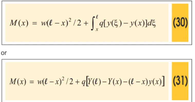
Figure 4-a shows the delected shape of a bar equivalent to a bracing system, subject to uniformly distributed loads of rates w and q, respec-tively in the horizontal and vertical directions; q is given by the sum of the rates p and v of igure 1-b. Taking into account the bar delections (geometric nonlinearity) and representing by Y the primitive function of the displacements y(x), the bending moment will be given by:
(30)
x
x
y
x
d
y
q
x
w
x
M
x
[
(
)
(
)]
2
/
)
(
)
(
=
l
-
2+
ò
l-or
(31)
[
(
)
(
)
(
)
(
)
]
2
/
)
(
)
(
x
w
x
2q
Y
Y
x
x
y
x
M
=
l
-
+
l
-
-
l
-Considering that y(0) = 0, the bending moment at support will be expressed by:
(32)
[
(
)
(
0
)
]
2
)
0
(
w
2q
Y
Y
M
=
l
+
l
-Figure 4 – Deformations influence in the structure response
Bracing system equivalent bar
BB
Shear deformation at the infinitesimal level4.1 Substructures of shear wall or shear core types
In the case of bracing systems formed exclusively by shear walls and/or shear cores, the differential equation of motion will be ob -tained equalizing
EJ
d
2y
/
dx
2 to M(x) given by (31):(33)
[
(
)
(
)
(
)
(
)
]
2
/
)
(
/
2 22
y
dx
w
x
q
Y
Y
x
x
y
x
d
J
E
=
l
-
+
l
-
-
l
-Deriving it in relation to x and considering that the rotations are given by f(x) = dy/dx, changes equation (33) into:
(34)
0
)
(
)
(
)
(
22
dx
+
q
-
x
x
+
w
-
x
=
d
J
E
f
l
f
l
An approximate solution for equation (34) can be obtained through the Galerkin method. Assuming that this solution is proportional to f(x) due exclusively to first order effects, it may be written:
(35)
ú
ú
û
ù
ê
ê
ë
é
÷
ø
ö
ç
è
æ
-=
=
1 1(
)
11
1
3)
(
l
x
a
x
a
x
j
f
where
ϕ
1(
x
)
was obtained deriving equation (14) in relation to x and suppressing the constant that would remain in evidence. Ap -plying equation (29) with n = 1, leads successively to:(36)
(
(
)
)
(
)
0
)
(
)
(
0 1 1 1
0
×
1=
ò
×
=
ò
lL
f
j
x
dx
lL
a
j
x
j
x
dx
(37)
( )
( )
ò
=
ú
ú
û
ù
ê
ê
ë
é
÷
ø
ö
ç
è
æ
-×
ïþ
ï
ý
ü
ïî
ï
í
ì
-+
ú
ú
û
ù
ê
ê
ë
é
÷
ø
ö
ç
è
æ
-+
÷
ø
ö
ç
è
æ
-ll
l
l
l
l
l
0 3 3 121
1
1
1
1
1
0
6
EJa
x
q
x
a
x
w
x
x
dx
Performing the integration and isolating a1, results:
(38)
33 1
24
EJ
4
w
l
3
q
l
a
-=
On substituting (38) into (35), the approximate solution is obtained:
(39)
ú
ú
û
ù
ê
ê
ë
é
÷
ø
ö
ç
è
æ
-=
3 31
1
33
24
4
)
(
l
l
l
x
q
EJ
w
x
f
Integrating (39) in relation to x and applying the condition of zero
displacement at support, leads to the displacements function. Inte-grating again, leads to:
(40)
C
x
x
x
q
EJ
w
x
Y
+
ú
ú
û
ù
ê
ê
ë
é
-+
÷
ø
ö
ç
è
æ
-=
l
l
l
l
l
5 23 4
2
1
5
3
24
)
(
where C is the integration constant. The bending moment at sup-port can be obtained on applying equations (32) and (40):
(41)
)
5(8
2
2
)
0
(
2 5 3l
l
l
q
EJ
qw
w
M
-+
=
Equation (41) can be transformed successively into:
(42)
3 3 2 3 3 28
5
/
8
2
)
5(8
4
1
2
)
0
(
l
l
l
l
l
l
q
EJ
q
EJ
w
q
EJ
q
w
M
-×
=
÷÷
ø
ö
çç
è
æ
-+
×
=
The condition of that, in the ultimate limit state (loads multiplied by 1,4), the second order effects may not exceed the irst order effects in more than 10% (inequality (1)), is applied to the support bending moment, obtaining:
(43)
2
1,4
1,1
1,4
8
/5
1,4
8
2
1,4
2 3 3 2l
l
l
l
w
q
EJ
q
EJ
w
£
´
-´
The terms wl2, multiplying both sides of the inequality, do vanish.
Performing the required algebraic transformations, results:
(44)
6349
,
0
/
3
EJ
£
ql
Since a wall or core has a behavior equivalent to the one of a column, the physical nonlinearity may be considered adopting for EJ the expression 0,941 ECSIC, according to equation (11). On the other hand, remembering that qlis the total vertical load Nk and lis the total height Htot, inequality (44) becomes:
(45)
5974
0,
/
CS C k2
tot
´
N
E
I
£
H
Extracting the square root of both members:
(46)
773
0,
/
CS Ck
Thus, inequality (46) denotes a value of 0,773 for a1. In its turn, the ABNT [8] code allows the coeficient a1 to be increased until 0,7 if the bracing system is composed exclusively by shear walls or shear cores.
4.2 Substructures of the rigid plane frame type
In the case of bracing systems formed exclusively by rigid frames, the equivalent bar of igure 4-a will deform predominantly by shear. Also in this case, the efforts expression must take the delected shape into account. It can be proved that the ininitesimals ds and dx shown in igure 4-b are related by:
(47)
2 2 2 2 22
+
=
(
1
+
)
=
1
+
f
=
dx
dy
dx
dy
dx
dx
ds
The shear effort can be obtained from the derivation of equation (31) in relation to the bar delected axis. Introducing ds given by (47), results:
(48)
)
(
1
)
(
)
(
)
(
)
(
1
)
(
2 2x
x
x
q
x
w
x
dx
dM
ds
dM
x
Q
f
f
f
+
-+
-=
+
-=
-=
l
l
It is an inclined shear effort, as shown in igure 4-b. The shear deforma -tion caused by it has the same slope, given at the ininitesimal level by:
(49)
2
2
1
1
1
cos
f
=
=
+
f
=
dy
+
f
dy
ds
dx
dy
dy
On establishing the differential equation of motion for this case, two changes must be performed with relation to equation (16): to introduce dy/cos f given by (49), in place of dy, and Q(x) given by (48). On doing so, results:
(50)
(x)
S
(x)
x)
q(
x)
w(
S
Q(x)
x
dx
dy
2 21
)
(
1
f
f
f
+
-+
-=
=
+
l
l
Thus:
(51)
)]
(
1
[
)
(
)
(
2x
S
x
x)
q(
x)
w(
dx
dy
x
f
f
f
+
-+
-=
=
l
l
In cases of “bland” geometric nonlinearity, as the ones treated by this work, the rotations f(x) present values much lesser than unit; therefore, f2(x) may be neglected in face of 1 and equation (51) may be put in the form:
(52)
)
(
)
(
)
(
)
(
x
w
x
q
x
x
S
f
=
l
-
+
l
-
f
Isolating f(x):
(53)
)
(
)
(
)
(
x
q
S
x
w
x
-=
l
l
f
Integrating equation (53) in relation to x and applying the condition of zero displacement at support, leads to the displacements func-tion. Integrating again, gives:
(54)
[
] [
{
]
}
(
x
)
C
q
w
)
q
(S
x
q
Sw
x)
q(
S
x)
q(
S
q
Sw
Y(x)
=
-
-
×
-
-
-
-
-
-
2+
2+
23
l
ln
l
1
ln
l
2
l
where C is the integration constant. Applying equation (54) for x = 0 and x = l, leads to the difference below:
(55)
÷÷
ø
ö
çç
è
æ
+
-=
-q
S
q
w
q
S
S
q
w
S
)
Y(
)
Y(
2
ln
0
23l
l
l
l
Thus, the bending moment at support can be expressed, substitut-ing equation (55) into (32):
(56)
q
Sw
S
q
ln
q
w
S
q
S
w
q
S
S
ln
q
w
S
w
)
M(
l
l
l
l
l
l
-=
÷÷
ø
ö
çç
è
æ
+
-+
=
/
1
1
2
2
0
2 22 22Applying the condition expressed by inequality (1) to this bending moment, results:
(57)
2
4
1
1
1
4
1
4
1
4
1
1
1
ln
4
1
4
1
2 2 22
l
l
l
w
,
,
q
,
Sw
,
S
q
,
q
,
w
S
,
-
£
´
-Performing the required algebraic transformations, inequality (57) changes into:
(58)
77
0
1
4
1
1
1
ln
4
1
1
2
,
q
/S
q
/S
,
/S)
(q
,
l
-
l
-
l
£
Taking the factor ql /Sas an unknown, inequality (58) can be solved by means of trials, obtaining:
(59)
0962
,
0
/
S
£
Substituting S by expression (18), results:
(60)
3848
0
2
×
q
l
/EJ
£
,
l
According to the ABNT [8] code, the physical nonlinearity might be considered, substituting EJ by (EI)sec given by (12). However, the (EI)sec /ECSIC ratio of the frame bars assemblage, as a function of the individual bar (EI)sec /ECSIC ratios cannot be considered a con-stant value; it can vary due to many factors, such as the numbers of loors and spans, story heights, span lengths, relation between the cross section dimensions of beams and columns etc. Pinto and Ramalho [11] show that the inluence of physical nonlinearity in the frame lateral stiffness depends mainly on the reinforcement ratios and the loading magnitude; they obtained (EI)sec /ECSIC ratios vary-ing from 0,51 until 0,75 for the ultimate limit state.
On the other hand, Schueler [12] states that the contribution of beams lexibility for the lateral delections of a rigid frame can reach 65%, remaining 35% due to columns lexibility. Furthermore, in a slender frame the beam reinforcements As and As’ tend to be the same, due to the predominance of wind effects. Thus, in this case equations (10) and (11) may be employed to relate the components of yNL (frame horizontal displacements including physical nonlinearity), due to the beams (yNLBEAMS) and columns (y
NL
COLUMNS), with the corresponding
components (yLBEAMS) and(y
LCOLUMNS) of the horizontal displacements resulting from linear analysis (yL). Simultaneously, the above-men -tioned share factors (35% and 65%) of these components in the total displacements may be used, leading to the following expressions:
(61)
941
,
0
35
,
0
941
,
0
L LNL
COLUMNS
COLUMNS
y
y
y
=
=
(62)
588
,
0
65
,
0
588
,
0
L LNL
BEAMS
BEAMS
y
y
y
=
=
Performing the sum of the components expressed by (61) and (62), leads to the following relation between the total horizontal displacements yNL and yL:
(63)
677
,
0
588
,
0
65
,
0
941
,
0
35
,
0
L L LNL
y
y
y
y
=
+
=
As the frame lateral stiffness is inversely proportional to these dis -placements, it may be written:
(64)
CCS
I
E
EI
)
0
,
677
(
sec=
Considering this expression of (EI)sec and following the same de-ductive sequence that led to the inequalities (45) and (46), results:
(65)
51
0,
/
CS C ktot
´
N
E
I
£
H
It can be noticed that this inequality is coherent with ABNT [8] code, which appoints the value of 0,5 for the coeficient a1, if the bracing system is constituted exclusively by rigid frames. In fact, in order to obtain a1 = 0,5, (EI)sec must satisfy the following:
(66)
CCi C
CS
I
E
I
E
EI
)
0
,
650
0
,
552
(
sec=
=
4.3 Associations of rigid frames with shear walls
and/or shear cores
The same model of igure 3 is adopted and the same deinitions of section 2.2 are considered. In order to deduce the differential equation of motion for the frames assemblage (igure 3-c), equa -tion (50) is applied, adding the terms due to the wall-frame interac -tion to the shear effort, as was done in equa-tion (19):
(67)
)
(
1
)
(
)
(
1
)
(
)
(
)
(
)
(
2 2
1 1
x
x
x
S
x
x
q
d
u
Q
x
w
S
Q(x)
T xf
f
f
f
x
x
+
=
+
-+
+
+
-=
l
ò
l
l
Considering that f2(x) may be neglected in face of 1 and isolating the terms due to the interaction forces:
(68)
)
(
)
(
)
(
)
(
)
(
d
S
x
w
1x
q
1x
x
u
Q
x
T
+
ò
x
x
=
f
-
l
-
-
l
-
f
l
In order to deduce the differential equation of motion for the walls assemblage (igure 3-b), the bending moment given by (31) is in -troduced, added to the terms due to the interaction forces, as was done in equation (21):
(69)
[
]
2222 2
2
(
)
(
()
)
)(
(
)
(
)
(
)
2
)
(
dx
y
d
EJ
x
y
x
x
Y
Y
q
d
x
u
x
Q
x
w
x
T
-
-
-
+
-
-
-
=
-ò
ll
l
l
l
x
x
x
Deriving equation (69) in relation to x, gives:
(70)
ò
-
-+
+
-=
=
l
ll
x
T
u
d
q
x
x
Q
x
w
dx
d
EJ
dx
y
d
EJ
2 2(
)
(
)
2(
)
(
)
2 2 3 3
Substituting (68) into (70) and re-arranging, results:
(71)
)
(
)
(
)
()
(
)
()
(
1 2 1 22 2
2
d
dx
w
w
x
q
q
x
x
S
x
EJ
f
=
-
+
l
-
-
+
l
-
f
+
f
Considering that w1 + w2 = w (total wind load), q1 + q2 = q (total gravity load) and re-arranging again, leads to the differential equa -tion describing the behavior of a system composed by rigid frames and walls/cores, including the delections inluence:
(72)
0
)
(
)
(
)]
(
[
2 22
d
dx
-
S
-
q
-
x
x
+
w
-
x
=
EJ
f
l
f
l
In order to apply the Galerkin method to equation (72), it will be assumed a solution given by a function f(x) multiplied by the linear solution, expressed by equations (25), (26) and (27):
(73)
ú
û
ù
ê
ë
é
-+
+
=
-(
)
4
)
(
)
(
1 2 / 2 2 / 21
e
C
e
w
EJ
x
C
x
f
x
Kxl Kx ll
l
f
Substituting (73) into (72), results:
(74)
+
ú
û
ù
ê
ë
é
-+
+
-(
)
4
)(
1 2 / 2 2 / 2 12
"f
x
C
e
C
e
w
EJ
x
EJ
Kxl Kxll
l
(
)
ú
+
(
+
)
-û
ù
ê
ë
é
--
- l l - ll
l
l
l
/ 2 2 / 2 1 2 2 2 1 2 / 2 2 / 2 12
)(
2
4
4
)(
2
Kx KxK
EJ
f
x
C
e
KxC
e
KxEJ
w
e
C
e
C
K
x'
f
EJ
[
]
(
)
(
)
0
4
)
(
)(
1 2 / 2 2 / 21
ú
+
-
=
û
ù
ê
ë
é
-+
+
--
-x
w
x
EJ
w
e
C
e
C
x
q
S
x
f
l
Kxl Kxll
l
l
Assuming that f(x) is a constant function, leads the irst and sec -ond terms of equation (74) to be null, since they are multiplied by the derivatives
f
'
(
x
)
andf
"
(
x
)
. Furthermore, considering the preceding deinitions of K (section 2.2) and S (equation 18), it may be written:(75)
S
EJ
EJ
K
=
=
21 2 2 2
4
4
l
l
Consequently, the third term of equation (74) cancels with some parts of the fourth one, reducing the equation to:
(76)
[
1
(
)
]
0
)
(
4
)
(
1 2 / 2 2 / 21
ú
+
-
=
û
ù
ê
ë
é
-+
+
-x
w
f
x
EJ
w
e
C
e
C
x
f
q
Kxl Kxll
l
The Galerkin method will be used in order to ind a constant func -tion
f
(x)
that has to be a good approximation for f(x) appearing in equation (76). According to (28), it may be written:(77)
1
)
(
)
(
1 11
'
=
=
a
x
x
(x)
f
j
j
For this case, equation (29) is applied in the following form:
(78)
[
]
{
(
)
4
1(
)
}
0
0 1 1
2 2 2 2 1
1
+
-
=
ò
la
q
C
e
Kx/l+ C
e
-Kx/lw
l
l
x
EJ
+ w
- a
dx
Performing the integration, a1 can be isolated, giving:
(79)
[
(
1
)
(
1
)
]
2
8
1
1
2 2 2 1 1 3 1-=
- KK
C
e
e
C
Kw
q
EJ
q
a
l
Therefore, the approximate solution for equation (72) will be given by:
(80)
ú
û
ù
ê
ë
é
-+
+
=
-(
)
4
)
(
1 2 / 2 2 / 2 11
C
e
C
e
w
EJ
x
a
x
Kxl Kxll
l
f
with a1 given by (79). Integrating twice leads to the primitive of the displacements function:
(81)
(
)
ú
û
ù
ê
ë
é
+
+
÷
ø
ö
ç
è
æ
-+
+
=
-4 3 1 2 2 / 2 2 / 2 1 2 21
4
4
2
6
)
(
x
C
x
C
EJ
x
w
e
C
e
C
K
a
x
Y
l
Kxl Kxll
l
where C4 is an undetermined constant and C3 results from the con-dition of zero displacement at support:
(82)
)
(e
K
e
)
K(e
EJ
w
C
K K K1
1
8
2 42 4
1 4
3
=
-
l
×
-
+
+
The bending moment at support is obtained, applying equation (32):
(83)
[
]
þ
ý
ü
î
í
ì
+
+
-+
-+
=
l
l
-l
l
3 1 5 2 2 2 1 2 2 1 2