SCALE OF OPERATION, ALLOCATIVE INEFFICIENCIES AND SEPARABILITY OF INPUTS AND OUTPUTS IN AGRICULTURAL RESEARCH
Geraldo da Silva e Souza
∗and Eliane Gonc¸alves Gomes
Received September 29, 2011 / Accepted April 24, 2013
ABSTRACT.In this article we consider some properties of concern for research production at Embrapa. We apply statistical tests to address questions related to the scale of operation, the presence of allocative inefficiencies and separability of inputs and outputs. The production process is assessed by nonparametric methods with the use of Data Envelopment Analysis. The period under analysis is 2002-2009. We conclude that Embrapa’s technology frontier shows variable returns to scale, is allocative efficient in general and is separable in inputs and outputs. These characteristics justify the company policy of adopting a VRS solu-tion and the aggregasolu-tion of output variables. Scale inefficiencies are the basis for further input congessolu-tion studies.
Keywords: DEA, efficiency, agricultural research.
1 INTRODUCTION
The Brazilian Agricultural Research Corporation (Embrapa) monitors, since 1996, the produc-tion process of 37 of its 42 research centers by means of a nonparametric producproduc-tion model. Measures of efficiency are computed using data envelopment analysis. For more details see Souza et al. (1999, 2007, 2010, 2011).
Our interest is on the economic, technical and allocative measures of efficiency, computed in the production system under the assumption of cost minimization. Several important questions arise in the actual application of DEA in the monitoring process at Embrapa.
Firstly there is the choice of aggregating or not the outputs. For some time Embrapa has used a weighted average of output variables as a single output indicator in its production model. Aggregation assumes separability, a property not fully investigated in the model. Aggregation in ultimate analysis is a consequence of a multicriteria additive model, which requires preferen-tial independence among the criteria (Pomerol & Barba-Romero, 2000; Bouyssouet al., 2010). From an economic point of view aggregation, as well as separability, has been a longstanding
*Corresponding author
subject of interest in the economic literature. See Berndt & Christensen (1973), Blackorbyet al. (1977), Chambers & F¨are (1993).
Secondly, there is the assumption on the scale of operation. Embrapa’s model imposes con-stant returns to scale, which generates harsh measures of efficiency for the evaluation process. The approach is justified by the measurement of inputs and outputs on a per employee basis. A statistical test is in order to quantify differences related to the scale of operation, if constant returns is to be used as the final choice in the evaluation model.
It is also of importance for the institution to identify the sources of economic inefficiencies. Are they due to technical inefficiencies, to poor choice of input combinations or both?
Our approach to test for the presence of allocative inefficiencies, returns to scale, and separability of inputs and outputs for Embrapa’s production system follows closely to Banker & Natarajan (2004).
Our discussion proceeds as follows. In Section 2 we describe Embrapa’s production system. In Section 3 we establish the technological nonparametric production setting that can be related to DEA and the parametric and nonparametric statistical tests that can be performed for the assessment of scale of production, allocative inefficiencies and separability. In Section 4 we show the empirical results based on the analysis by year. Finally, in Section 5 we summarize our results.
2 EMBRAPA’S RESEARCH PRODUCTION MODEL
Embrapa’s research system currently comprises 42 research centers (DMUs in the DEA context). Five of these production units were recently created and are not included in the evaluation system. For this reason, our sample consists of 37 DMUs. Input and output variables have been defined from a set of performance indicators known to the company since 1991. The company uses routinely some of these indicators to monitor performance through annual work plans. With the active participation of the board of directors of Embrapa, as well as the administration of each of its research units, 28 output and three input indicators were selected as representative of production actions in the company.
The output indicators were classified into four categories: Scientific Production; Production of Technical Publications; Development of Technologies, Products, and Processes; Diffusion of Technologies and Image.
By Scientific Production we mean the publication of articles and book chapters. We require that each item be specified with complete bibliographical reference. Specifically, the category of Scientific Production includes the following items:
1. Scientific articles published in refereed journals and book chapters – domestic publica-tions1.
2. Scientific articles published in refereed journals and book chapters – foreign publications1.
1Prior to the definition of the categories’ weights, the different types of articles are combined following the QUALIS/
CAPES classification. The weights used in this aggregation were defined by Embrapa’s administration as follows:
3. Articles and summaries published in proceedings of congresses and technical meetings.
The category of Production of Technical Publications groups publications produced by research centers aiming, primarily, agricultural businesses and agricultural production. Specifically,
1. Technical circulars. Serial publications, written in technical language, listing recommen-dations and information based on experimental studies. The intended coverage may be the local, regional or national agriculture.
2. Research bulletins. Serial publications reporting research results.
3. Technical communiqu´es. Serial publications, succinct and written in technical language, intended to report recommendations and opinions of researchers in regard to matters of interest to the local, regional or national agriculture.
4. Periodicals (document series). Serial publications containing research reports, technolog-ical information or other matter not classified in the previous categories. Examples are proceedings of technical meetings, reports of scientific expeditions, reports of research programs etc.
5. Technical recommendations/instructions. Publication written in simplified language aimed at extensionists and farmers in general, and containing technical recommendations in re-gard to agricultural production systems.
6. Ongoing research. Serial publication written in technical language and approaching as-pects of a research problem, research methodology or research objectives. It may convey scientific information in objective and succinct form.
The category of Development of Technologies, Products and Processes groups indicators related to the effort made by a research unit to make its production available to society in the form of a final product. We include here only new technologies, products and processes. These must be already tested at the client’s level in the form of prototypes, through demonstration units or be already patented. Specifically,
1. Cultivars. Plants varieties, hybrids or clones.
2. Agricultural and livestock processes and practices.
3. Agricultural and livestock inputs. All raw materials, including stirps, that may be used or transformed to obtain agricultural and livestock products.
4. Agro-industrial processes. Operations carried out at commercial or industrial level envis-aging economic optimization in the phases of harvest, post harvest and transformation and preservation of agricultural products.
6. Scientific methodologies.
7. Software.
8. Monitoring, zoning (agro ecologic or socioeconomic) and mapping.
Finally, the category of Diffusion of Technologies and Image encompasses production actions related with Embrapa’s effort to make its products known to the public and to market its image. Here we consider the following indicators:
1. Field days. The research units organize these events. The objective is the diffusion of knowledge, technologies and innovations. The target public is primarily composed of farmers, extensionists, organized associations of farmers (cooperatives), and under-graduate students. The field day must involve at least 40 persons and last at least four hours.
2. Organization of congresses and seminars. Only events with at least three days of duration time are considered.
3. Seminar presentations (conferences and talks). Presentation of a scientific or technical theme within or outside the research unit. Only talks and conferences with a registered attendance of at least 20 persons and duration time of at least one hour are considered.
4. Participation in expositions and fairs. Participation is considered only in the following cases: (a) With the construction of a stand with the purpose of showing the center’s research activities by audiovisuals and distributing publications uniquely related to the event’s theme; (b) Co-sponsorship of the event.
5. Courses. Courses offered by a research center. Internal registration is required specifying the course load and content. The course load should be at least eight hours. Disciplines offered as part of university courses are not considered.
6. Trainees. Concession of college level training programs to technicians and students. Each trainee must be involved in training activities for at least 80 hours to be counted in this item.
7. Fellowship holders. Orientation of students (the fellowship holders). The fellowship dura-tion should be at least six months and the workload at least 240 hours.
8. Folders. Only folders inspired by research results are considered. Re-impressions of the same folder and institutional folders are not counted.
10. Demonstration units. Events organized to demonstrate research results – technologies, products, and processes – already in the form of a final product, in general with the co-participation of a private or governmental agent of technical assistance.
11. Observation units. Events organized to validate research results, in space and time, in commercial scale, before the object of research has reached its final form. Observations units are organized in cooperation with producers, cooperatives, and other agencies of research or private institutions. The events may be organized within or outside the re-search unit.
The input side of Embrapa’s production process is composed of three factors:
1. Personnel costs. Salaries plus labor duties.
2. Operational costs. Expenses with consumption materials, travels and services, less income from production projects.
3. Capital. Measured by depreciation.
As indicators of the production process we consider a system of dimensionless relative indices. These are all quantity indexes. The idea, from the output point of view, is to define a combined measure of output as a weighted average of the relative indicators (indices). The relative indices are computed for each production variable and for each research unit within a year dividing the observed production quantity by the mean per research unit. The input indices are indicated by xio,i =1,2,3. These quantities represent relative indices of personnel, operational expenditures and capital expenditures, respectively.
Output measures per category are defined as follows. The output componentyi,i=1,2,3,4, of each production category is a weighted average of the relative indices composing the category. Ifois the DMU (research unit) being evaluated then
yoi =
ki
j=1
aoj iyoj i; 0≤aoj i;
ki
j=1
aoj i =1
whereaoj i, j =1, . . . ,ki is the weight system for DMUoin the category of productioni,ki is the number of production indicators comprisingiandyoj iis the relative index of production j.
The weights, in principle, are supposed to be user defined and should reflect the administra-tion’s perception of the relative importance of each variable to each DMU. Defining weights is a hard and questionable task. In our application we followed an approach based on the law of categorical judgment of Thurstone (1927). See Torgerson (1958) and Kotz & Johnson (1989). It is an alternative to the AHP method of Saaty (1994). The model is well suited when several independent judges are involved in the evaluation process.
m ≥ 2 categoriesC = {C1, . . . ,Cm}. A referee or judge, randomly chosen from a population, is to classify each stimulus Si into one of the categoriesCj. The categories inC are mutu-ally exclusive and ordered according to an underlying characteristic of interest. In this context C1 < C2 <· · · <Cm represents the ordination inC, that is, relative to the characteristics of interestC1represents the least intense impulses andCmthe most intense impulses.
Each time a referee faces a stimulus, a mental discriminal process is put into action and it gen-erates a numerical value in the real line reflecting the stimulus intensity. Therefore, in this way, the stimuli translate in the psychological continuum into scale valuesµ1, . . . , µr. Likewise the categories translate into location valuesτ1, . . . , τm−1. These later quantities form a partition of
the real line(−∞, τ1], (τ1, τ2], . . . , (τm−1,+∞]. The partition relates to stimuli S1and
cate-goriesCj according to the following rule. The referee classifies stimulusSi into∪lj=1Cl if and only ifµi ≤ τj. The process inherits randomness from the sampling scheme and from the fact that due to stochastic fluctuations in nature, a given stimulus and category when repeatedly eval-uated by a referee does not generate the same scale and boundary values in the psychological continuum. Randomness leads one to assume that theµi are indeed means of random variables ξiwith varianceσi2and thatτjare indeed means of random variablesηj with variancesφ2j. The discussion imposes row independence and joint normality, that is, theξi are uncorrelated and (ξ, ηj)are jointly normally distributed. In principle, one has primary interest in the pairwise parametric differencesµi−µj.
Letπi j denote the probability of locating stimulusSi into one of the first j categoriesC1,C2,
. . . ,Cj. We assumeπi j >0. We then have (1).
P
Si ∈ j
l=1
Cl
= πi j, i=1, . . . ,r, j =1, . . . ,m−1
= P{ξi ≤ηj} =
Z ≤ − µi −τj Var(ξi −ηj)
.
(1)
Letg(·)denote the probit transformation. The assumption of joint normality leads to the equa-tions (2), relating the cumulative probabilitiesπi j to the parameters of Thurstone’s model.
g(πi j)= −
µi −τj
Var(ξi −ηj)
, i =1, . . . ,r, j=1, . . . ,m−1. (2)
Clearly it is possible to generalize the normal projection on the psychological continuum to other distributions. Any monotonic function may play the role of g(·). Typical alternatives in this context would be the logistic scale g(x) = ln{x/(1 −x)}and the log-log scale g(x) = ln{−ln(1−x)}. Here we follow the logistic scale.
If enough observations are available to estimate the probabilitiesπi j in (2), then the sample version of the Law of Categorical Judgment is therefore (3), whereπˆi jis the relative cumulative frequency of observations in categoryCj.
g(πˆi j)= −
µi −τj
Var(ξi −ηj)
The vectorsu′i =(ui1, . . . ,uim−1)are independently distributed with a distinct variance matrix
for eachi. Clearly,πˆi j = ˆpi1+ ˆpi2+ · · · + ˆpi j, where pilrepresents the proportion of times the referees classify stimulusSiintoCl.
We follow a particular case of this specification known as Model B (Torgenson, 1958; McCullagh & Nelder, 1989). Model B assumes Var(ξi −ηj) = δi. From (3), this assumption generates the nonlinear regression model (4).
g(πˆi j)= − µi−τj
δi
+εi j. (4)
Notice that we must have 2r+m−3 ≤ r(m −1), i.e., the number of parameters should be at most the number of observations. The number of parameters is adjusted for two identifying restrictions r
i=1δ1i =r and r
i=1µδii =0.
Following Souza (2002), the relative importance of stimuliiis given by (5), assuming the logis-tic scale.
1−πi j
πi j
δi
r
v−1
1−πiv
πiv
δv . (5)
The parameters needed to use this formula may be estimated by maximum likelihood using the multinomial distribution or generalized least squares (GLS) assuming residuals centered at zero. We followed the GLS approach.
We sent out about 500 questionnaires to researchers and administrators and asked them to rank in importance – scale from 1 to 5 – each production category and each production variable within the corresponding production category. A set of weights was determined under the assumption that the psychological continuum of the responses projects onto a lognormal distribution.
centers. It is important to emphasize here that we are postulating a production model. The uni-variate yis assumed to be a monotonic concave function of the inputs defined on a convex set of a three dimensional space. We assume separability, on economic and multicriteria senses, to aggregate outputs. Separabilty will be tested.
We see the use of ratios to define production variables in our application as unavoidable. Dif-ferent denominators are used with the virtue of being independent of the units’ size. This char-acteristic facilitates comparisons between units and allows the assumption of a common pro-duction function. In the context of a pure DEA analysis, the problem of efficiency comparisons may be resolved by imposing the BCC assumption. See Hollingsworth & Smith (2003) and Emrouznejad & Amin (2009). These authors state that when using ratio variables, the constant returns to scale assumption is not valid. In this context a comparison of CCR and BCC solutions is in order.
DEA models are known to be sensitive to outliers. Here we recognize two types of outliers: errors of measurement, mainly in the output variables, and benchmarks resulting from the DEA analysis. We want to detect DEA (benchmarks) outliers. Errors of measurement are undesirable. In our application is crucial the control of this type of error. Control of measurement errors out-liers prior to the DEA analysis is particularly important for output variables to avoid spurious efficiency scores. In this context we use box plot fences to identify the values of outlying obser-vations. Following standard exploratory statistical practices (Hoaglinet al., 2000), values above Q3+1.5(Q3−Q1)are investigated and acted upon if indeed resulted from measurement error. HereQ1 andQ3 denote the first and third quartiles, respectively.
3 TECHNOLOGY SET AND DEA ESTIMATION
Letxj ≥ 0 and yj ≥ 0, j = 1, . . . ,n, be the observed input and output vectors in a sample ofn observations generated from the underlying technology set T = {(x,y); output ycan be produced from inputs x}. The underlying technology T is convex and satisfies the properties listed in Coelliet al. (2005). The efficiency of a DMU jis defined by (6).
θ (xj,yj)=infnη;(ηxj,yj)∈T. (6)
Bankeret al. (2011) assume the following minimal additional probabilistic structure. The quan-tity θ is modeled as a random variable with probability density f(θ ) with support in(0,1). It is further assumed that ifδ ∈(0,1), then1
δ f(θ )dθ >0.
Under the above assumptions the estimatesθ (ˆ xj,yj)are consistent and converge in distribution, whereθ (ˆ xj,yj)=minλ,ηη, subject to the conditionsYλ≥ yj,Xλ≤ηxj,λ1=1 andλ≥0. HereY =(y1, . . . ,yn)is the output matrix andX =(x1, . . . ,xn)is the input matrix.
Banker & Natarajan (2004) suggest three statistical tests to examine the assumption constant versus variable returns to scale. Two of them are based on specific assumptions on the den-sity function f(θ )(exponential and half-normal distributions), and the third is a nonparametric test. Our choice is for the nonparametric test, which is based on the Smirnov-Kolmogorov two sample statistics.
Discussions about returns to scale in DEA can be seen, for instance, in F¨are & Grosskopf (1994), Zhu & Shen (1995), Jahanshahlooet al. (2005), Sueyoshi & Sekitani (2007), Djivre & Menashe (2010), Krivonozhkoet al. (2011), Khaleghiet al. (2012), Soleimani-Damaneh (2012), Essidet al. (2013).
Now we turn our attention to separability of inputs and outputs. We begin with complete input separability. The technology set under this assumption becomes (7). Here s is the number of inputs andxgis a particular coordinate, andxs−1the remaining components of thes-vectorx.
TSinp=
s
g=1
TinpSepg; TinpSepg =
(x =(xg,xs−1),y);xgmay producey. (7)
For output separability we have (8). Herel is the number of outputs and yg is one particular coordinate, andyl−1the remaining components of thel-vectory.
TSoutp=
l
g=1
Toutg
Sep; T
outg
Sep =
(x,y=(yg,yl−1),y);xgmay produceyg
. (8)
Under the assumption of separability of inputs, the efficiency of firm j is given by (9).
θSinp(xj,yj)=infηη;(ηxj,yj)∈TSinp (9)
It can be proved that
θSinp(xj,yj)= max g=1...s
θ (xgj,yj), where θ (xgj,yj)=infηη;(ηxj,yj)∈TSinpg.
Under separability of inputs the efficienciesθSinp(xj,yj)can be estimated calculating a DEA coefficient under constant or variable returns to scale considering, in turn, a DEA estimate
ˆ
θ (xj,ygj)for each input, and computing the maximum of these measurements. One obtains a similar estimate under output separability computing the DEA estimates for each output and the maximum of these measurements. The statistical assessment of separability is performed again via Smirnov-Kolmogorov test statistic.
The separability condition has also been studied by Homburg (2005), Kuosmanenet al. (2006), Ajalliet al. (2011).
to be compared via a nonparametric statistical test like the Smirnov-Kolmogorov two sample test. We notice here that technical efficiency information may be retrieved from cost data on inputs as in Banker & Natarajan (2004).
Allocative efficiencies were studied by Sueyoshi (1992), Fukuyama & Weber (2002, 2003), Ruiz & Sirvent (2011), Paradi & Tam (2012), Begumet al. (2012), among others.
4 EMPIRICAL RESULTS
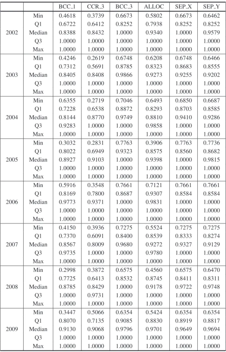
Table 1 shows descriptive statistics for the efficiency measurements of concern in our study. These are cost efficiencies (BCC 1), technical efficiencies under constant returns to scale (CCR 3), technical efficiencies under variable returns to scale (BCC 3), allocative efficiencies (ALLOC) and technical efficiencies computed under the assumptions of separability of inputs (SEP X) and outputs (SEP Y), respectively. Orientation in all DEA models is for inputs and technical efficiencies are computed, typically, with four outputs and three inputs. Cost efficien-cies are calculated with four outputs and one input (aggregated cost).
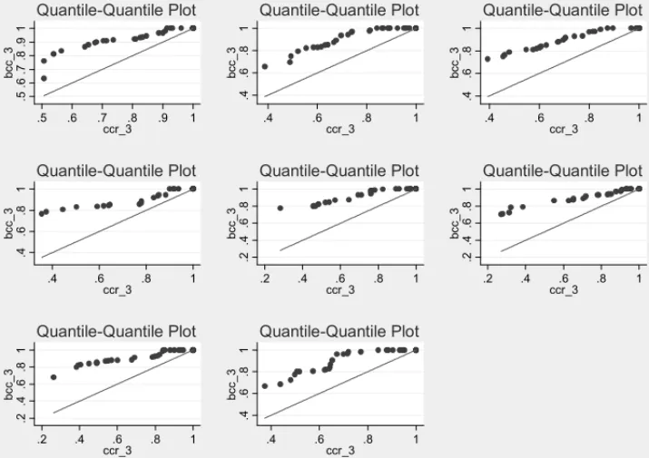
Looking at medians and quartiles we see large differences regarding the assumptions of scale. These differences are further highlighted in Figure 1, where one sees other quantiles under each assumption quite distinct. In the context of formal statistical test, only in 2006 the Smirnov-Kolmogorov statistics shows a non significant p-value of 13.4%. Even in this case Figure 1 shows a distortion from the null hypothesis of no scale effect.
As a referee pointed out, a DMU that has a minimum input value for any input item or a max-imum output value for any output item is BCC-efficient. This is a characteristic of the DEA analysis under the VRS assumption. We notice that the theoretical production model considered in this article does not allow the presence of fully efficient DMUs. This property does not affect consistency and distributional results of the efficiency score relative to the underlying population technology. In practical applications the weights on the optimum solution should be examined in search of Pareto optimality. When one is concerned in characterizing factors causing efficiency, efficient units may simply be discarded from the analysis, as in Simar & Wilson (2007), or mod-eled via a fractional regression, as in Ramalhoet al. (2010, 2011). If the BCC score is viewed as a performance index and one is worried about spurious efficiency derived from unreasonable input or output measurements, the scenario may be detected before the efficiency analysis by robust statistical methods of outlier detection.
Table 1– Number summaries for cost efficiency (BCC 1), technical efficiency under constant returns to scale (CCR 3), variable returns to scale (BCC 3), allocative efficiency (ALLOC) and technical efficiencies under separability for inputs (SEP X) and outputs (SEP Y).
BCC 1 CCR 3 BCC 3 ALLOC SEP X SEP Y
Min 0.4618 0.3739 0.6673 0.5802 0.6673 0.6462
Q1 0.6722 0.6412 0.8252 0.7938 0.8252 0.8252
2002 Median 0.8388 0.8432 1.0000 0.9340 1.0000 0.9579
Q3 1.0000 1.0000 1.0000 1.0000 1.0000 1.0000
Max 1.0000 1.0000 1.0000 1.0000 1.0000 1.0000
Min 0.4246 0.2619 0.6748 0.6208 0.6748 0.6466
Q1 0.7312 0.5691 0.8785 0.8323 0.8683 0.8555
2003 Median 0.8405 0.8408 0.9866 0.9273 0.9255 0.9202
Q3 1.0000 1.0000 1.0000 1.0000 1.0000 1.0000
Max 1.0000 1.0000 1.0000 1.0000 1.0000 1.0000
Min 0.6355 0.2719 0.7046 0.6493 0.6850 0.6687
Q1 0.7228 0.6538 0.8872 0.8293 0.8703 0.8585
2004 Median 0.8144 0.8770 0.9749 0.8810 0.9410 0.9286
Q3 0.9283 1.0000 1.0000 0.9858 1.0000 1.0000
Max 1.0000 1.0000 1.0000 1.0000 1.0000 1.0000
Min 0.3032 0.2831 0.7763 0.3906 0.7763 0.7736
Q1 0.8022 0.6949 0.9323 0.8575 0.8560 0.8682
2005 Median 0.8927 0.9103 1.0000 0.9398 1.0000 0.9815
Q3 1.0000 1.0000 1.0000 1.0000 1.0000 1.0000
Max 1.0000 1.0000 1.0000 1.0000 1.0000 1.0000
Min 0.5916 0.3548 0.7661 0.7121 0.7661 0.7661
Q1 0.8169 0.7800 0.8687 0.9307 0.8584 0.8584
2006 Median 0.9773 0.9371 1.0000 0.9831 1.0000 1.0000
Q3 1.0000 1.0000 1.0000 1.0000 1.0000 1.0000
Max 1.0000 1.0000 1.0000 1.0000 1.0000 1.0000
Min 0.4150 0.3936 0.7275 0.5524 0.7275 0.7275
Q1 0.7370 0.6091 0.8400 0.8539 0.8333 0.8274
2007 Median 0.8567 0.8009 0.9680 0.9272 0.9327 0.9129
Q3 0.9735 1.0000 1.0000 0.9780 1.0000 1.0000
Max 1.0000 1.0000 1.0000 1.0000 1.0000 1.0000
Min 0.2998 0.3872 0.6575 0.4560 0.6575 0.6470
Q1 0.7725 0.6413 0.8532 0.8745 0.8411 0.8311
2008 Median 0.8785 0.8429 1.0000 0.9178 0.9722 0.9748
Q3 1.0000 0.9731 1.0000 1.0000 1.0000 1.0000
Max 1.0000 1.0000 1.0000 1.0000 1.0000 1.0000
Min 0.3447 0.5066 0.6354 0.5424 0.6354 0.6354
Q1 0.8070 0.7135 0.9085 0.8830 0.8919 0.8817
2009 Median 0.9130 0.9068 0.9796 0.9701 0.9649 0.9694
Q3 1.0000 1.0000 1.0000 1.0000 1.0000 1.0000
.5 .6 .7 .8 .9 1 b cc_ 3
.5 .6 .7 .8 .9 1
ccr_3 Quantile-Quantile Plot .4 .6 .8 1 b cc_ 3
.4 .6 .8 1
ccr_3 Quantile-Quantile Plot .4 .6 .8 1 b cc_ 3
.4 .6 .8 1
ccr_3 Quantile-Quantile Plot .4 .6 .8 1 bc c _ 3
.4 .6 .8 1
ccr_3 Quantile-Quantile Plot .2 .4 .6 .8 1 bc c _ 3
.2 .4 .6 .8 1
ccr_3 Quantile-Quantile Plot .2 .4 .6 .8 1 bc c _ 3
.2 .4 .6 .8 1
ccr_3 Quantile-Quantile Plot .2 .4 .6 .8 1 bc c _ 3
.2 .4 .6 .8 1
ccr_3 Quantile-Quantile Plot .4 .6 .8 1 bc c _ 3
.4 .6 .8 1
ccr_3
Quantile-Quantile Plot
Figure 1– Quantile-quantile plots of technical efficiency measures under variable returns to scale (BCC 3) and constant returns to scale (CCR 3) by year – 2009 to 2002 in row order.
.6 .7 .8 .9 1 se p _ x
.6 .7 .8 .9 1
bcc_3 Quantile-Quantile Plot .6 .7 .8 .9 1 se p _ x
.6 .7 .8 .9 1
bcc_3 Quantile-Quantile Plot .7 .8 .9 1 se p _ x
.7 .8 .9 1
bcc_3 Quantile-Quantile Plot .7 5 .8 .8 5 .9 .9 5 1 se p _ x
.75 .8 .85 .9 .95 1
bcc_3 Quantile-Quantile Plot .7 5 .8 .8 5 .9 .9 5 1 se p _ x
.75 .8 .85 .9 .95 1
bcc_3 Quantile-Quantile Plot .7 .8 .9 1 se p _ x
.7 .8 .9 1
bcc_3 Quantile-Quantile Plot .7 .8 .9 1 se p _ x
.7 .8 .9 1
bcc_3 Quantile-Quantile Plot .6 .7 .8 .9 1 se p _ x
.6 .7 .8 .9 1
bcc_3
Quantile-Quantile Plot
.6 .7 .8 .9 1 se p _ y
.6 .7 .8 .9 1
bcc_3 Quantile-Quantile Plot .6 .7 .8 .9 1 se p _ y
.6 .7 .8 .9 1
bcc_3 Quantile-Quantile Plot .7 .8 .9 1 se p _ y
.7 .8 .9 1
bcc_3 Quantile-Quantile Plot .7 5 .8 .8 5 .9 .9 5 1 se p_ y
.75 .8 .85 .9 .95 1
bcc_3 Quantile-Quantile Plot .7 5 .8 .8 5 .9 .9 5 1 se p_ y
.75 .8 .85 .9 .95 1
bcc_3 Quantile-Quantile Plot .6 .7 .8 .9 1 se p_ y
.7 .8 .9 1
bcc_3 Quantile-Quantile Plot .6 .7 .8 .9 1 se p_ y
.7 .8 .9 1
bcc_3 Quantile-Quantile Plot .6 .7 .8 .9 1 se p_ y
.6 .7 .8 .9 1
bcc_3
Quantile-Quantile Plot
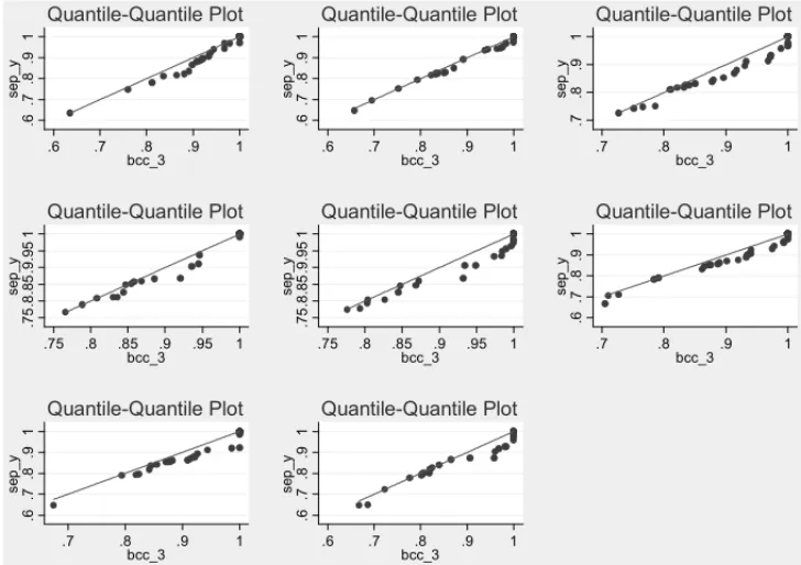
Figure 3– Quantile-quantile plots for investigation of output separability by year – 2009 to 2002 in row order. SEP Y is technical efficiency under output separability and variable returns to scale and BCC 3 is technical efficiency under variable returns to scale.
The differences between the use of separate and combined outputs can be seen in the median efficiency evolution in the period 2002-2009. For separate outputs the figures are 1.00, 0.99, 0.97, 1.00, 1.00, 0.97, 1.00, 0.98, respectively, and for a weighted average combined output the figures are as expected lower: 0.90, 0.85, 0.87, 0.89, 0.91, 0.87, 0.88, and 0.88, respectively. These differences do not seem to be strong enough to invalidate statistically the separability assumption.
There are statistically significant allocative inefficiencies for almost all years. Correspondingp -values for Smirnov Kolmogorov test statistics are 1%, 0.4%, 0.03%, 7.6%, 13.4%, 7.6%, 7.6%, 4% for years 2002-2009, respectively. On the other hand, it should be pointed out that the annual medians of allocative efficiencies are all above 90% (exception of 2004 with 88%), indicating proper choices of input mixes. In this case the Smirnov-Kolmogorov test statistics seems to be detecting small deviations.
5 CONCLUSIONS AND EXTENSIONS FOR FUTURE STUDIES
For Embrapa’s research production model we investigated the properties of returns to scale, proper choice of input mixes and separability of inputs and outputs.
The assumption of constant returns to scale is rejected leading to the more flexible variable returns assumption and higher values of the DEA measures of efficiency. The scale adjustments carried out by the company were not successful to overcome scale of operation differences.
Allocative efficiency is very high for all years, although one notices, in sub-periods, statistically significant differences relative to a variable returns cost technology frontier.
Inputs and outputs are separable. This implies that aggregation is justifiable on both sides of production. The implications of this result to Embrapa are important. For inputs, separability means that the influence of each of the inputs on the output is independent of the other inputs, emphasizing the need for controlling marginal input effects. For outputs, it implies that the same efficiency level could be obtained considering as a production response an output projection on a lower dimensional space. In this context, combined output weighted averages may be computed to impose administration perceptions in the production process and to reduce any biases noticed in the process in the direction of an unwanted grouping of variables. This justifies the use of combined outputs by the company in the evaluation process.
Future researches, as a result of the studies carried out here, should envisage the association of scale inefficiencies with congestion measures. Coelliet al. (2005) points out that one should not go looking for congestion, as it will often be found whether or not it actually exists. Scale is an important component in congestion studies.
ACKNOWLEDGMENTS
The authors would like to thank the National Council for Scientific and Technological Develop-ment (CNPq) for the financial support.
REFERENCES
[1] AJALLIM, BAYATN, MIRMAHALLEHSRS & RAMAZANIMRM. 2011. Analysis of the technical efficiency of the provincial gas companies in Iran making use of the synthetic model of Data Envel-opment Analysis and Anderson-Peterson Method (DEA-AP).European Journal of Social Sciences, 25(2): 156–160.
[2] BANKERRD & NATARAJANR. 2008. Evaluating contextual variables affecting productivity using data envelopment analysis.Operations Research,56(1): 48–58.
[3] BANKERRD & NATARAJANR. 2004. Statistical tests based on DEA efficiency scores. In: COOPER WW, SEIFORDLM & ZHUJ. (Eds.). Handbook on Data Envelopment Analysis, Kluwer Interna-tional Series, Boston, 299–321.
[5] BEGUMIA, ALAM MJ, BUYSSEJ, FRIJAA &VANHUYLENBROECKG. 2012. Contract farmer and poultry farm efficiency in Bangladesh: A data envelopment analysis. Applied Economics, 44(28): 3737–3747.
[6] BERNDTER & CHRISTENSENLR. 1973. The internal structure of functional relationships: separa-bility, substitution and aggregation.The Review of Economic Studies,40(3): 403–410.
[7] BLACKORBY C, PRIMONT D & RUSSELL RR. 1977. On testing separability restrictions with flexible functional forms.Journal of Econometrics,5(2): 195–209.
[8] BOUYSSOUD, MARCHANT T, PIRLOT M, TSOUKIASA & VINCKE P. 2010. Evaluation and Decision Models with Multiple Criteria: stepping stones for the analyst. Springer, New York.
[9] CHAMBERSRG & F ¨ARER. 1993. Input-output separability in production models and its structural consequences.Journal of Economics,57(2): 197–202.
[10] COELLITJ, RAODSP, O’DONNELLCJ & BATTESEGE. 2005. An Introduction to Efficiency and Productivity Analysis. 2ndedition. Springer, New York.
[11] DJIVREJ & MENASHEY. 2010. Testing for constant returns to scale and perfect competition in the Israeli economy, 1980-2006.Israel Economic Review,8(2): 67–90.
[12] EMROUZNEJAD A & AMINRAG. 2009. DEA models for ratio data: convexity consideration. Applied Mathematical Modelling,33(1): 486–498.
[13] ESSID H, OUELLETTE P & VIGEANTS. 2013. Small is not that beautiful after all: Measuring the scale efficiency of Tunisian high schools using a DEA-bootstrap method.Applied Economics Volume,45(9): 1109–1120.
[14] F ¨ARER & GROSSKOPFS. 1994. Estimation of returns to scale using data envelopment analysis: A comment.European Journal of Operational Research,79(2): 379–382.
[15] FUKUYAMA H & WEBER WL. 2002. Estimating output allocative efficiency and productivity change: Application to Japanese banks.European Journal of Operational Research,137(1): 177– 190.
[16] FUKUYAMAH & WEBER WL. 2003. Modeling input allocative efficiency via distance and quasi-distance functions.Journal of the Operations Research Society of Japan,46(3): 264–285.
[17] HOAGLINDC, MOSTELLERF & TUKEYJW. 2000. Understanding Robust and Exploratory Data Analysis. Wiley, New York.
[18] HOLLINGSWORTHB & SMITHP. 2003. Use of ratios in data envelopment analysis.Applied Eco-nomics Letters,10(11): 733–735.
[19] HOMBURGC. 2005. Using relative profits as an alternative to activity-based costing.International Journal of Production Economics,95(3): 387–397.
[20] JAHANSHAHLOO GR, SOLEIMANI-DAMANEH M & ROSTAMY-MALKHALIFEH M. 2005. An enhanced procedure for estimating returns-to-scale in DEA. Applied Mathematics and Computa-tion,171(2): 1226–1238.
[21] KHALEGHIM, JAHANSHAHLOOG, ZOHREHBANDIANM & LOTFIFH. 2012. Returns to scale and scale elasticity in two-stage DEA. Mathematical and Computational Applications,17(3): 193–202.
[23] KRIVONOZHKO VE, FØRSUND FR & LYCHEV AV. 2012. Returns-to-scale properties in DEA models: the fundamental role of interior points.Journal of Productivity Analysis,38(2): 121–130.
[24] KUOSMANENT, PEMSLD & WESSELERJ. 2006. Specification and estimation of production func-tions involving damage control inputs: A two-stage, semiparametric approach.American Journal of Agricultural Economics,88(2): 499–511.
[25] MCCULLAGH P & NELDER JA. 1989. Generalized Linear Models. 2nd edition. Chapman & Hall/CRC, London.
[26] PARADIJC & TAMFK. 2012. The examination of pseudo-allocative and pseudo-overall efficien-cies in DEA using shadow prices.Journal of Productivity Analysis,37(2): 115–123.
[27] POMEROL JC & BARBA-ROMERO S. 2000. Multicriterion decision in management: Principles and practice. Kluwer Academic, Boston.
[28] RAMALHOEA, RAMALHOJJS & HENRIQUESPD. 2010. Fractional regression models for second stage DEA efficiency analyses.Journal of Productivity Analysis,34(3): 239–255.
[29] RAMALHO EA, RAMALHO JJS & MURTEIRA JMR. 2011. Alternative estimating and testing empirical strategies for fractional regression models.Journal of Economic Surveys,25(1): 19–68.
[30] RUIZJL & SIRVENTI. 2011. A DEA approach to derive individual lower and upper bounds for the technical and allocative components of the overall profit efficiency.Journal of the Operational Research Society,62(11): 1907–1916.
[31] SAATY TL. 1994. The Fundamentals of Decision Making and Priority Theory with the Analytic Hierarchy Process. RWS Publication, Pittsburgh.
[32] SEIFORDLM & THRALLRM. 1990. Recent developments in DEA, the mathematical program-ming approach to frontier analysis.Journal of Econometrics,46(1-2): 7–38.
[33] SIMARL & WILSONPW. 2007. Estimation and inference in two-stage, semi-parametric models of production processes.Journal of Econometrics,136(1): 31–64.
[34] SOLEIMANI-DAMANEHM. 2012. On a basic definition of returns to scale.Operations Research Letters,40(2), 144–147.
[35] SOUZAGS. 2002. The law of categorical judgement revisited.Brazilian Journal of Probability and Statistics,16(2): 123–140.
[36] SOUZA GS, AVILA AFD & ALVES E. 1999. Technical efficiency of production in agricultural research.Scientometrics,46(1): 141–160.
[37] SOUZAGS, GOMESEG & STAUBRB. 2010. Probabilistic measures of efficiency and the influence of contextual variables in nonparametric production models: an application to agricultural research in Brazil.International Transactions in Operational Research,17(3): 351–363.
[38] SOUZAGS, GOMESEG, MAGALHAES˜ MC & AVILAAFD. 2007. Economic efficiency of Embrapa research centers and the influence of contextual variables.Pesquisa Operacional,27(1): 15–26.
[39] SOUZAGS, SOUZAMO & GOMESEG. 2011. Computing confidence intervals for output oriented DEA models: an application to agricultural research in Brazil.Journal of the Operational Research Society,62: 1844–1850.
[41] SUEYOSHIT & SEKITANIK. 2007. Measurement of returns to scale using a non-radial DEA model: A range-adjusted measure approach.European Journal of Operational Research,176(3): 1918–1946.
[42] THURSTONELL. 1927. A law of comparative judgments.Psychological Review,34(4): 273–286.
[43] TORGERSONWS. 1958. Theory and Methods of Scaling. Wiley, New York.