Abstract
Some mineral deposits show mineralization along layers. These layers may pass through several subsequent geological events such as folding and/or severe erosional pro-cesses. Grades within these deposits tend to be correlated along orientations where the mineralization was originally deposited or along the same geological period (stratigraphic level). Consequently, some locations close to each other in terms of geographical coordi-nates can show uncorrelated grades. Spatial continuity analysis can also be affected by er-ror inlicted by combining samples from different stratigraphic levels. This article uses the coordinate transformation (unfolding) to align the grades measured along the same strati-graphic level. The modiication in coordinates improved the spatial continuity modeling and the grade estimates at non-sampled locations. The results showed that the mean of the relative error between the estimated value and the real value of the samples using unfolding is -0.10%. However, when using the original coordinates, the mean of the relative error is -0.65%. Furthermore, the correlation between the real and estimated value using cross-validation is greater using stratigraphic coordinates. A complete case study in a manganese deposit illustrates the methodology.
keywords: Change of coordinates, stratigraphic coordinates, grade estimation, kriging.
Ricardo Hundelshaussen Rubio
Engenheiro Industrial, MSc, Doutorando, Universidade Federal Rio Grande do Sul, Departamento de Engenharia de Minas, Porto Alegre, Rio Grande do Sul, Brasil [email protected]
Vanessa Cerqueira Koppe
Professora Auxiliar,
Engenheira de Minas, MSc, Dra. em Engenharia Universidade Federal Rio Grande do Sul, Departamento de Engenharia de Minas, Porto Alegre, Rio Grande do Sul, Brasil [email protected]
João Felipe Coimbra Leite Costa
Professor,Engenheiro de Minas, MSc, PhD, Universidade Federal Rio Grande do Sul, Departamento de Engenharia de Minas, Porto Alegre, Rio Grande do Sul, Brasil [email protected]
Pablo Koury Cherchenevski
Engenheiro de Minas, MSc,
Universidade Federal Rio Grande do Sul, Departamento de Engenharia de Minas, Porto Alegre, Rio Grande do Sul, Brasil [email protected]
How the use of
stratigraphic coordinates
improves grade estimation
Mining
Mineração
http://dx.doi.org/10.1590/0370-44672015680057
1. Inroduction
Mineral deposits such as baux-ite, coal, manganese and some nickel laterites are constituted mainly by large mineralized layers. These layers formed by sedimentation or weath-ering processes may pass through several subsequent geological events such as folding, erosions and/or basin formation.
One of the most common prob-lems for this kind of deposit is the spatial continuity analysis. This spatial continuity may be affected by an error caused by the combination of samples from different stratigraphic levels. For example, two samples may be in the same topographic or Cartesian
level but along a different geologic or stratigraphic horizon. Figure 1 (a) shows that the Cartesian coordinates of samples 1 and 4 are at the top and at the bottom of the mineralized layer respectively, however at the same z – topographic coordinate. The analysis of the spatial continuity and the block estimates would benefit if samples deposited along the same geologic horizon were used; therefore, Sample 1 should have more spatial connectiv-ity with Sample 2 than with Sample 4 (see Figure 1b).
The geostatistical modeling is based on the spatial dependence of the samples. In this type of strata-bound
Figure 1
Interpretation of coordinates between different samples, (a) Cartesian coordinates (b) stratigraphic coordinates.
The objective of this paper is to evaluate the possible beneits in terms of
increasing the precision and accuracy of the estimates with the change of
coor-dinates. A manganese deposit is used to illustrate the methodology.
2. Methodology
In the 80s and 90s, some authors demonstrated interest in using strati-graphic coordinates (Rendu and Readdy, 1982; Weber, 1982-1990; Dagbert et al.,
1984; Bashore and Araktingi, 1994). McArthur (1988) used the transfor-mation of Cartesian coordinates into stratigraphic coordinates in a uranium deposit in Australia, assigning arbitrarily stratigraphic numbers to the new vertical coordinate Z. Since then, a few studies
have shown the process systematically to transform Cartesian coordinates into stratigraphic coordinates in a real case study; among them we ind a real case of sonic wave slowness in Koppe et al.,
(2006). Other alternatives to the unfold-ing techniques can be considered such as geostatistics with locally varying Anisot-ropy (Boisvert et al., 2009).
Deutsch (2002) suggests some approximations that can be made to
transform Cartesian coordinates into stratigraphic coordinates. A vertical coordinate will be deined as the relative distance between a correlation top and correlation base grid. This will make it possible to infer natural measures of horizontal correlation and to preserve the geologic structure in the inal numerical model (Deutsch, 2002). The new vertical coordinates can be calculated using the following equation:
where:
Z(i)str = Z elevation after stratigraphic correction in sample (i);
Z(i) = actual Z elevation in sample (i); Z(i)b = bottom layer Z elevation in sample (i);
Z(i)t = top layer Z elevation in sample (i);
T = average layer thickness;
n = number of samples.
This article considered that the mineralized layer has slight changes in
thickness along its extension (i.e. Z(i)t-Z(i)
b ≅ T), therefore, the equation suggested
by Deutsch (2002) has been redeined as follows:
Equations 2 and 3 represent the stratigraphic coordinates performed using as references the footwall and hangwall distance correction respectively. The new vertical coordinate transformations will be a plane shape, maintaining the distances between horizontal coordinates (Cartesian coordinates).
This transformation, does not cor-rect the horizontal distances between samples, which can, in cases where the layers are folded strongly, modify the horizontal continuity determined by the samples values, leading to errors in the determination of the variograms. There-fore, the use of this transformation is
appropriate for deposits that show only a slight folding along of the layers. Figure 2 shows the transformation of a stratiform geological layer whose coordinates on the vertical axis (Figure 2a) are transformed to stratigraphic coordinates corrected by the footwall (Figure 2b) or hangwall (Figure 2c) of the layer.
i = 1,...,n
i = 1,...,n
i = 1,...,n
Z(i)
str=
Z(i) - Z(i)
bZ(i)
t- Z(i)
bT
*
(1)(2) (3) Z(i)str = Z(i) - Z(i)b
Z(i)str = Z(i)t - Z(i)
Figure 2 Example of a stratiform layer,
(a) Cartesian geological, (b) stratigraphic coordinates corrected by the footwall of the layer, (c) stratigraphic coordinates corrected by the hangwall of the layer. The change of coordinates is made only on the vertical axis (Z).
Figure 3 shows the spatial distribu-tion of the original data in the plane YZ.
Note that, the stratiform geological layer has a slight folding along the deposit.
Figure 3 Base map of the samples distribution in the plane YZ.
This article begins with a com-parison between two point estimates (footwall and hangwall) to choose which reference surface is the most
adequate. Subsequently, we will ana-lyze the spatial continuity and point estimates between original Cartesian coordinates and stratigraphic
coordi-nates. Finally, we will make an esti-mate in blocks to validate the results of the proposed methodology.
3. Results
3.1 Case Study
The case study corresponds to a data set from a manganese deposit located in the Brazilian Amazon (Figure 4).
Figure 4 Location map of the study area.
(a)
3.2 Selection of the Surface of Reference
In order to evaluate the two cor-rections and choose the one that will be used in the analysis of spatial continuity and estimation, two datasets with a new vertical coordinate along Z (distance to hangwall or footwall) were created. Cross-validation (Isaaks and Srivastava, 1989) was used to check the quality of the estimates for the two coordinate-transformed datasets. Figure 5 (a) showsthat the mean error of the variable man-ganese (mn1) corrected by the hangwall is closer to zero (-0.12) compared with the mean error of the same variable (Figure 5 (b)) corrected by the footwall (-0.55). Furthermore, the spread around the mean error was lower using the hangwall. Con-sequently, it was decided to proceed with the stratigraphic coordinates corrected by the hangwall.
Due to the difference in the sample support (variables analyzed in different granulometric fractions), it was necessary to proceed with an auxiliary (accumulat-ed) variable of the manganese. At the end of the estimation process, the accumula-tion is divided by the mass fracaccumula-tion at each block to return unbiased grade estimates (Marques et al., 2014). Furthermore, the jackknife cross validation was performed.
Figure 5
Histogram of distribution of error, (a) coordinates correct by the hangwall, (b) coordinates corrected by the footwall.
3.3 Spatial Continuity Analysis
The spatial continuity for the man-ganese was obtained using experimental non ergodic correlograms (Srivastava, 1987). The construction of these models was performed using data at the original Cartesian coordinates as well as at thestratigraphic coordinates. Figure 6 shows the models adjusted to the major horizon-tal directions of anisotropy for each data coordinate. Note that, the modeling using stratigraphic coordinates (Figure 6c, d) produces better structured experimental
correlograms than when using Cartesian coordinates (Figure 6a, b). The noise noted in the experimental correlogram using Cartesian coordinates (Figure 6a, b) is due to the inluence of events subsequent to the formation of the deposit.
Figure 6
Models of spatial continuity using Carte-sian coordinates
(a) major axis N-90 dip 0
(b) intermediate axis N-0 dip 0 and, using stratigraphic coordinates
(c) major axis N-90 dip 0 (d) intermediate axis N-0 dip 0.
(a) (b)
(a) (b)
3.4 Validation of Estimates points Using Original Coordinates and Stratigraphic Coordinates
A comparison was made using crossvalidation (Isaaks and Srivastava, 1989) to check the results by the coordinate trans-formation and using the originals. The method consists of removing momentarily a sample positioned at the location (u) from the original dataset. This location (u) is estimated using the information of the remaining samples and, inally, the dif-ference between the estimated value and the actual value at the same location (u) is calculated. This difference is known as the error of cross validation. The process is repeated for all samples in the dataset.
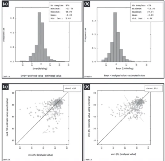
Figures 7a and 7b show the error histogram for the estimates using both the Cartesian coordinates and the strati-graphic coordinates. Note that the mean error using stratigraphic coordinates (Fig-ure 7b) is close to zero (-0.10) whilst the mean error using Cartesian coordinates is -0.65 (Figure 7a). Furthermore, the spread of the error around the center is smaller when using stratigraphic coordinates.
Likewise, Figures 8a and 8b show the scatterplot between the two estimates (original vs. unfolding). Note that the cor-relation between real and estimated value
using stratigraphic coordinates (Figure 8b) is 0.50 whilst the correlation between real and estimated value using Cartesian coordinates is 0.45 (Figure 8b). Globally this difference may be insigniicant, but we can see that the dispersion of the esti-mated values in relation to real value using unfolding (Figure 8b) is much less than the estimated values estimated in the Carte-sian coordinates (Figure 8a). For example, the estimated values in red are closer when using stratigraphic coordinates (Figure 8b) than when using Cartesian coordinates (Figure 8a).
Figure 7 Error histograms obtained by cross validation using (a) original Cartesian coordinates and (b) stratigraphic coordinates correction.
Figure 8 Correlations obtained by cross validation using (a) original Cartesian coordinates and (b) stratigraphic coordinates correction.
3.5. Validation of Estimates Blocks Using Stratigraphic Coordinates
The first check used to verify themodels is the reproduction of the global declustered mean of the original data. Figure 9 shows the histogram of declustered data (Figure 9a) obtained using the polygonal method (Isaaks and Srivastava, 1989) and histogram of the estimated data (Figure 9b) obtained by ordinary kriging (Matheron, 1963). Note that the global mean of the estimates (47.19%) is very similar to the
declustered mean (47.15%), with a slight relative difference of 0.08% between the two, thus ensuring a good reproduction by the estimated model.
Next, the local means were checked. Basically, this method consists in locally comparing the values of the declustered mean and the kriged block model for each attribute along bands in the X, Y and Z directions. The result of each mean is
plot-ted versus its location along X, Y and Z. The plots of the local mean show coherence between both estimates along each band. Figures 10 (a, b, c) show the swath plots between the estimated blocks and declus-tered data along the three main directions, i.e. X, Y, and Z. Note that the local mean estimates are very similar to the declustered mean along each band. The bands used were 100 m wide along X and Y and 8 m along Z. When mixing samples from different
stratigraphic levels, the grades lose spatial connectivity, since they are a result of a
sampling mix that was probably not de-posited along the same deposition period (different horizons). This leads to bias and
noise when calculating the experimental spatial continuity and ultimately leading to incorrect spatial continuity.
(a) (b)
Figure 9
Validation of global mean, (a) declustered data histogram (b) block model grades histogram using the stratigraphic coordinates.
Figure 10
Swath plot for the manganese, (a) X direction,
(b) Y direction and
(c) Z. Red line represents the declustered mean from the data and black line represents the estimated blocks.
4. Conclusion
Stratiform deposits are frequently found in different mineral commodities, and they are properly modelled and es-timated in most cases. Coordinate cor-rection along the vertical axis (Z) using stratigraphic coordinates is essential in geostatistical estimations for this style of mineralization. Ignoring this practice leads to a mix between samples from different geochemical horizons possibly not correlated and ultimately leading to
a signiicant bias in the estimates. The use of stratigraphic coordi-nates showed to be more appropriate for properly capturing the spatial ity. Correlograms were more continu-ous with greater adhesion between the experimental points and the model, if compared to the ones using Cartesian coordinates. Furthermore, the error de-rived by comparing the estimated values and the actual values was more precise
and accurate when using stratigraphic coordinates than when using Cartesian coordinates. Moreover, the correlation between the real and estimated value using cross-validation is greater using stratigraphic coordinates.
The global and local means in the estimated grade block model using stratigraphic coordinates is very similar to the global and local means using declustered data.
5. References
BASHORE, W. M., ARAKTINGI, U.G. Importance of a geological framework and seismic data integration for reservoir modeling and subsequent luid-low. In: CO-BURN, T.C., YARUS, J. M., CHAMBERS, R. L.(Ed.). Stochastic modeling and
(a) (b)
(a) (b)
Received: 08 April 2015 - Accepted: 02 September 2015.
geostatistics: principles, methods and case studies. AAPG Computer Applications in Geology, n. 5, p. 159-176, 1994.
BOISVERT, J., MANCHUK, J., DEUTSCH, C V. Kriging and simulation in the pre-sence of locally varying anisotropy. Mathematical Geosciences, v. 41, n. 10, p. 585-601. 2009.
DAGBERT, M., DAVID, M., CROZEL, D., DESBARATS, A. Computing vario-grams in folded strata-controlled deposits. In: VERLY, G. et al. (Ed.). Geostati-sitcs for Natural Resources Characterization. D. Reidel, Dordrecht., p. 71-89. 1984. (Part 1).
DEUTSCH, C. V. Geostatistical reservoir modeling. New York: Oxford University Press, , 2002. 376p.
ISAAKS, E. H., SRIVASTAVA, M. R. An introduction to applied geostatistics. New York: Oxford University Press, , 1989. 561p.
KOPPE, V. C. Análise de incerteza associada à determinação da velocidade de onda sônica em depósitos de carvão obtida por perilagem geofísica. Porto Alegre: Uni-versidade Federal Rio Grande do Sul, 2005. 282p.
KOPPE, C. V., COSTA, J. F., KOPPE, J. C. Coordenadas cartesianas x coordenadas geológicas em geoestatística: aplicação à variável vagarosidade obtida por perila-gem acústica. REM - Revista Escola de Minas, v. 59, n. 1, p. 25-30, 2006. MATHERON, G. Principles of geostatistics. Economic Geology, n. 58, p.
1246-1266, 1963.
MCARTHUR, G. J. Using geology to control geostatistics in the Hellyer deposit. Ma-thematical Geology, v. 20, n. 4, p. 343-366, 1988.
MARQUES, D. M., HUNDELSHAUSSEN, R. J., COSTA, J. F., APPARICIO, E. M. The effect of accumulation in 2D estimates in phosphatic ore. REM - Revista Escola de Minas, v. 67, n. 4, p. 431-437, 2014.
RENDU, J. M., READDY, L. Geology and the Semivariogram. A Critical Rela-tionship. In: APCOM SYMPOSIUM, 17. New York: A.I.M.E., 1992, p. 771-783. SRIVASTAVA, R. M. Non-ergodic framework for variogram and covariance
func-tions. Stanford, CA: Stanford University, 1987. (Master’s Thesis).
WEBER, K. J. Inluence of common sedimentary structures on luid low in reservoirs models. Journal of Petroleum Technology, v. 34, p. 665-672, 1982.