ISSN 0101-8205 www.scielo.br/cam
On hydromagnetic rotating flow of a dusty fluid
near a pulsating plate
SANCHITA GHOSH1 and ARUN K. GHOSH2
1Department of Computer Science, BIT Mesra, Ranchi 835215, India 2Department of Mathematics, Jadavpur University, Kolkata, 700032, India
E-mail: [email protected]
Abstract. An initial value problem is solved for the motion of an incompressible viscous
conducting fluid with embedded small inert spherical particles bounded by an infinite rigid non-conducting plate. Both the plate and the fluid are in a state of solid-body rotation with constant angular velocity about an axis normal to the plate. The unsteady flow is generated in the fluid-particle system due to velocity tooth pulses subjected on the plate in presence of a transverse magnetic field. It is assumed that no external electric field is imposed on the system and the magnetic Prandtl number is very small. The operational method is used to derive exact solutions for the fluid and the particle velocities and the shear stress at the wall. Some limiting cases of these solutions including the steady-state results are discussed. The general solutions for the fluid velocity and the wall shear stress are examined numerically and the simultaneous effects of rotation, the magnetic field and the particles on them are determined. Finally, the present result for the fluid velocity has been compared numerically with that generated by an impulsively moved plate in a particular case when time is large.
Mathematical subject classification: 76U05.
Key words: hydromagnetic, pulsatile flow, rotating dusty fluid.
1 Introduction
The fluid flow generated by pulsatile motion of the boundary is found to have immense importance in aerospace science, nuclear fusion, astrophysics, atmo-spheric sciences, cosmical gasdynamics, geophysics, and physiological fluid
oscillations to multiple frequency unidirectional pulsatile motion with a view to its application in the analysis of suspension boundary layers in a rotating sys-tem [13], the motion in the liquid core of the earth which is responsible for the observed maintenance and secular variation of the mean geomagnetic field [14], the development of sunspot, the solar cycle and the structure of the magnetic stars [15] and in the flow and heat transfer characteristics of a fluid film over a rotating surface which is important in a number of industrial applications such as spreading of protective coating on electronics and optical devices, lithography and ablation cooling [16].
The problem is concerned with the unsteady flow developed in a semi-infinite expanse of an incompressible electrically conducting viscous fluid containing uniformly distributed small inert spherical particles bounded by an infinite rigid non-conducting plate in presence of an external magnetic field acting transversely to the plate when both the plate and the fluid are in a state of solid-body rotation with constant angular velocity about an axis normal to the plate and the plate is subjected to velocity tooth pulses impulsively from rest. The inquiries are made about the exact solutions for the fluid and the particle velocities and the shear stress at the wall. The results are computed numerically with a view to disclose the quantitative response of various flow parameters on the components of fluid velocity and the wall shear stress. The ultimate steady-state boundary layers are discussed. The present result for the fluid velocity at large values of time has been compared numerically with that generated by impulsively moved plate. It is seen that, in presence of pulsation, particles increase the fluid velocity near the plate only when rotation is small and time is large which is not the case in absence of pulsation. Finally, many known results are derived as limiting cases of the present solutions.
2 Mathematical formulation
external magnetic fieldBare in usual notations:
∂u
∂t +(u· ∇)u+2×u = − 1
ρ∇p+ν∇ 2
u
+ K N
ρ (v−u)+ 1
ρ(j×B)
(2.1)
m
∂v
∂t +(v· ∇)v+2×v
=K(u−v) (2.2)
∇ ·u=0 and ∂N
∂t + ∇ ·(Nv)=0 (2.3a,b)
whereu=(u1,u2,u3)andv =(v1, v2, v3)represent the velocities of the fluid and the particles respectively, p is the fluid pressure, N is the number density of the particles which are distributed uniformly in the fluid of densityρand kinematic viscosityν, m is the mass of the particle,K is the Stokes’ resistance coefficient which for spherical particles of radius a is 6π µa,jis the current density,Bis the magnetic flux density, andis the angular velocity of the coordinate system.
The Maxwell equations with usual MHD approximation are:
∇ ·B=0, ∇ ×B=µ0j, ∇ ×E= −∂B
∂t, (2.4)
j=σ0(E+u×B) (2.5)
where the displacement currents are neglected,µ0andσ0are constants andEis the electric field.
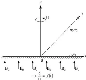
Figure 1 – Geometry of the flow configuration.
We assume that the magnetic Prandtl number Pm = σ0µ0ν << 1 which is plausible for most electrically conducting fluids and no electric fieldEis imposed on the system. This implies that the current is mainly due to induced electric field so thatj=σ0(u×B)and the applied magnetic field is essentially unaltered by the electric current flowing through the fluid. We further assume that the induced magnetic field produced by the motion of the fluid is negligible compared to the applied magnetic field so that Lorentz force term in (2.1) becomes −σ0
ρ B 2 0u. Moreover, the particles are uniformly distributed in the fluid and the flow field is parallel to the x-direction. This implies that all the physical variables are functions of z and t only and the equation (2.3b) is satisfied throughout the flow field whenN =N0= constant.
On the basis of the assumptions made above, the unsteady motion of a two-phase fluid-particle system occupying the semi-infinite spacez >0 is governed by the equations:
∂q
∂t +2iq =ν ∂2q ∂z2 +
k
and
∂r
∂t +2ir = 1
τ(q−r) (2.7)
whereq =u1+i u2is the complex fluid velocity, andr =v1+iv2is the complex particle velocity,k= m N0
ρ is the ratio of the mass density of the particles and the fluid density, usually called, the mass concentration of the particles,τ = mK is the relaxation time of the particles andn= σ0
ρ B 2
0 is the hydromagnetic parameter. Introducing the non-dimensional variables
(q′,r′)= (q,r) U , z
′= √z
ντ and t
′= t
τ (2.8)
and the non-dimensional flow parameters
E =2τ , n′=nτ (2.9)
in equations (2.6) and (2.7) and dropping the primes, we get the non-dimensional equations of motion in the form
∂q
∂t +i Eq = ∂2q
∂z2 +k(r −q)−nq (2.10) and
∂r
∂t +i Er =q−r. (2.11)
The above equations are to be solved subject to the boundary and initial condi-tions given by
q(o,t)= f(t), t >0, (2.12)
(q,r)−→(0,0) as z−→ ∞, t >0, (2.13a,b)
(q,r)=(0,0) at t ≤0 for all z, (2.14a,b)
where f(t) represents the tooth pulses which is an even periodic function of time with period 2T and strength E1T.
3 Solution of the problem
In view of the nature of f(t)mentioned above the mathematical form ofq(o,t) may be written as
q(0,t)= E1 T
t H(t)+2
∞
p=1
(−1)p(t−pT)H(t−pT)
whereH(t)is the Heaviside step function defined as
H(t−T)=0,t<T and H(t−T)=1,t ≥T. (3.2)
Using half-range Fourier series the condition (3.1) may also be written as
q(0,t)= E1 2 −
4E1 π2
∞
p=0
cos
(2p+1)πt/T
(2p+1)2 . (3.3) We now use Laplace transform to the equations (2.10) and (2.11) subject to initial conditions given in(2.14a,b). The transformed equation for the fluid velocity then becomes
d2q¯ d z2 −
(S+i E+1)(S+i E+k+n)−k S+i E +1
¯
q =0 (3.4)
with
¯
q −→0 as z −→ ∞ (3.4a)
and
¯ q = E1
T S2tanh
ST
2 at z =0 (3.4b)
whereSis the Laplace transform variable. The solution of (3.4) gives
¯
q(z,S)= E1 T S2tanh
ST 2 exp −z
(S+i E +c)(S+i E+d) S+i E +1
21 (3.5)
where
c,d = 1 2
a1+n±a12+2n(a1−2)+n2
1
2 (3.6a,b)
with a1=1+k and c≥a1≥1>d. The inversion of (3.5) yields
q(z,t)= E1
T
γ+i∞
γ−i∞
tanh
ST 2
S2 exp
St−z
(S+i E+c)(S+i E+d)
S+i E+1
12
d S (3.7)
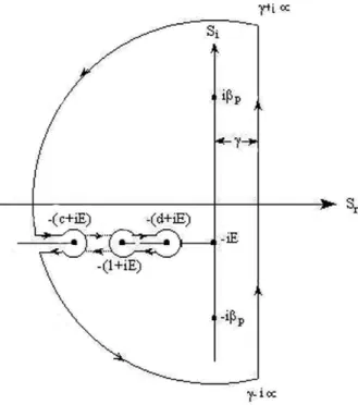
Figure 2 – Contour for the integral(3.7).
On evaluation of the integral (3.7) with the help of residue theorem applied to the contour shown above, the solution forq(z,t)comes out as
q(z,t) E1 =
1 2exp
−√z
2(L1+i L2)
− 2
T2
∞
p=0
1 β2
p
eiβptexp
−√z
2(M1+i M2)
+ e−iβptexp
−√z
2(N1±i N2)
− e
−i Et
πT
∞,1
c,d
e−xttanh[(x +i E)T/2] (x +i E)2
× Sin
z
(x−c)(x−d) x −1
12 d x
where
L1,L2 = (1+E2)−
1
2± [cd+E2(c+d−1)]
+ {cd+E2(c+d−1)}2+E2(c+d−cd+E2)2 1 2
1 2,
(3.9a,b)
M1,M2 = (1+(E+βp)2)−
1
2± [cd+(E+βp)2(c+d−1)]
+ {cd+(E+βp)2(c+d−1)}2+(E+βp)2 × (c+d−cd+(E+βp)2)2
1 2
1 2,
(3.10a,b)
N1,N2 = (1+(E−βp)2)−
1
2± [cd+(E−βp)2(c+d−1)]
+ {cd+(E−βp)2(c+d−1)}2+(E−βp)2 × (c+d−cd+(E−βp)2)2
1 212
,
(3.11a,b)
∞,1 c,d =
∞
c +
1 d
and±signs in (3.8) represent the casesE > βpandE < βp
respectively.
The particle velocity for the corresponding motion can be determined from (2.11) as
r(z,t)=e−(1+i E)t t
0
q(z, ξ )e(1+i E)ξ dξ (3.12) which on using (3.8) yields
r(z,t)
E1 =
exp−√z
2(L1+i L2)
{1−e−(1+i E)t}
2(1+E2)21
e−iφ1
− 2
T2
∞
p=0
exp−√z
2(M1+i M2)
β2
p(1+ E+βp 2)
1 2
eiβpt
−e−(1+i E)te−iφ2
+
∞
p=0
exp−√z
2(N1±i N2)
β2
p(1+ E−βp 2)
1 2
e−iβpt −e−(1+i E)te−iφ3
+e
−i Et
πT
∞,1
c,d
tanh[(x+i E)T/2] (x+i E)2
e−xt −e−t
x−1
× Sin
z
(
x−c)(x−d)
x−1
12
d x
where tanφ1= E,tanφ2=E+βpand tanφ3= E−βp.
Thus the exact solutions for the fluid velocityq(z,t)and the particle velocity r(z,t)are described in equations (3.8) and (3.13) respectively.
4 Limiting cases
( i )The unsteady flow generated in the existing system due to impulsively moved plate can be obtained by making the time periodT −→0 which in turn makes the frequency of pulsationβp −→ ∞. In this situation, the modified forms of the fluid and the particle velocities, as obtained from (3.8) and (3.13) are
q(z,t)
E1 =
1 2exp
−√z
2(L1+i L2)
− e
−i Et
2π ∞,1
c,d
e−xt
(x+i E)Sin
z
(
x−c)(x−d)
x−1
12
d x,
(4.1)
r(z,t)
E1 =
exp−√z
2(L1+i L2)
{1−e−(1+i E)t}
2(1+E2)12
e−iφ1
+ e
−i Et
2π ∞,1
c,d
e−xt−e−t
(x+i E)(x−1)Sin
z
(
x−c)(x−d)
x−1
12
d x.
(4.2)
On putting E1 = 2, the fluid velocity corresponding to Rayleigh problem for hydromagnetic rotating flow in a two-phase fluid can be obtained from (4.1) as
q(z,t) = exp
−√z
2(L1+i L2)
− e
−i Et
π
∞,1
c,d
e−xt (x +i E)Sin
z
(x−c)(x−d) x−1
12 d x,
(4.3)
( ii )For the clean fluid (k = 0), the result (3.8) gives the fluid velocity in the form
q(z,t) E1 =
1 2exp
−√z
2(α1+iα2)
− T22
∞
p=0
1 β2 p exp
iβpt− z √
2(m1+i m2)
+ exp
−iβpt− z √
2(n1±i n2)
− e
−i Et
πT
∞
n
tanh[(x+i E)T/2] (x+i E)2 Sin
z√x−ne−xtd x
(4.4)
where
α1, α2 =
(n2+E2)1/2±n1/2, m1,m2 =
(n2+ E +βp 2)1/2±n 1/2
,
n1,n2 = (n2+ E −βp 2)1/2±n 1/2
.
The result (4.4) is a new one and describes the fluid velocity for the hydromagnetic rotating flow of a viscous fluid near a pulsating plate.
Further, when T −→ 0, E1 = 2 and E = 0, (4.4) provides the solution of hydromagnetic Ekman problem as
q(z,t) = exp
−√z
2(α1+iα2)
− e
−i Et
π ∞
n
e−xt x+i E Sin
z√x −nd x.
(4.5)
This result in the limitn −→0 yields
q(z,t)= 1 2
ez
√
i E er f c
z
2√t +
√
i Et
+e−z
√
i E er f c
z
2√t −
√
i Et (4.6)
which agrees perfectly with Thornley’s [18] result (5.2) withc =1.
Finally, in the limitt −→ ∞, (4.6) recovers the classical Ekman layer solution
q(z,t)=e−z
√
i E
and in absence of rotation (E = 0), it approaches to well-known Rayleigh solution
q(z,t)=er f c
z
2√t . (4.8)
( iii )The solutions of the present problem in a non-rotating system(E =0)are given by
q(z,t)
E1 =
1 2e
−z√cd − 4
T2
∞
p=0
1 β2
p
e−γ1z/ √
2
Cos(βpt−γ2z/ √
2)
− 1
πT
∞,1
c,d
e−xttanh(x T/2)
x2 Sin
z
(
x−c)(x−d)
x−1
1/2
d x,
(4.9)
and
r(z,t) E1 =
1 2e
−z√cd
(1−e−t)
− T22
∞
p=0
e−γ1z/ √
2 β2
p
eiβpt−e−t
1+iβp
e−iγ2z/ √
2
+ e
−iβpt −e−t 1−iβp
eiγ2z/ √
2
+ 1
πT
∞,1
c,d
tanh(x T/2) x2
e−xt−e−t (x−1)
× Sin
z
(x −c)(x −d) x−1
1/2 d x
(4.10)
where
γ1, γ2 = 1+β2p −1/2
±
cd+β2p(c+d−1)
+
cd+β2p(c+d−1)2
+β2p
c+d−cd+β2p21/21/2 .
(4.11a,b)
The results (4.9) and (4.10) are the same as those of Ghosh and Ghosh [10]. WhenT −→0 andE1=2, we get
q(z,t)=e−z
√
cd − 1
π
∞,1
c,d e−xt
x Sin
z (x
−c)(x−d) x−1
1/2
and
r(z,t) = e−z√cd (1−e−t)+ 1 π
∞,1
c,d e−xt
−e−t x(x−1)
× Sin
z (x
−c)(x−d) x−1
1/2 d x.
(4.13)
These results are in complete agreement with Yang and Healy [19] corresponding to their case ω −→ 0 (impulsively moved plate) and describe the solutions for the fluid and the particle velocities associated with Stokes problems for a conducting fluid with suspension of particles.
Further, on puttingk=0 (clean fluid) in (4.12), we find the fluid velocity cor-responding to hydromagnetic Rayleigh problem in a non-rotating system which is mentioned in Pai [20]. The solution for the fluid velocity in this case is given by
q(z,t) = e−z√n − 1 π
∞
n e−xt
x Sin
z√x −nd x
= 1 2
e−z√ner f cη−√nt +ez√ner f cη+√nt
(4.14)
whereη= z 2√t.
Finally, in the hydrodynamic limit(n → 0), (4.14) approaches the classical Rayleigh layer solution
q(z,t)=er f cη (4.15)
which is same as derived in (4.8).
( iv )The complex flow given by (3.8) and (3.13) attains the steady-state in the limit t→ ∞ and the ultimate flow field comprises of
q(z,t) E1 =
1 2exp
− √z
2(L1+i L2)
− T22
∞
p=0
1 β2
p
eiβptexp
−√z
2(M1+i M2)
+e−iβptexp
−√z
2(N1±i N2)
and
r(z,t) E1 =
exp −√z
2(L1+i L2) 2(1+E2)12
e−iφ1
− 2 T2 ∞ p=0
exp
iβpt−√z
2(M1+i M2) β2
p(1+ E+βp 2)
1 2
e−iφ2
+
∞
p=0
exp−iβpt−√z2(N1±i N2) β2
p(1+ E−βp 2)
1 2
e−iφ3
(4.17)
It follows from (4.16) and (4.17) that the particles in the steady-state are unable to attain the actual fluid velocity due to the presence of rotation and pulsation. But in the limitT →0, E1=2 and E =0, we haveu1=v1. This shows that, in absence of pulsation and rotation, the particles attain the fluid velocity in the steady motion generated by impulsively moved plate. This result is also known from Michael and Miller’s [21] analysis.
It is also noticed from (4.16) that the ultimate flow consists of distinct multiple boundary layers, commonly known as Stokes-Ekman Hartman layers, whose thickness are of order
1 M1
√
2ντ , 1 L1
√
2ντ , 1 N1
√
2ντ where M1>L1>N1. (4.18) These boundary layers are modified by rotation, the magnetic field and the par-ticles.
However, in the limit T → 0, E1 = 2 and E = 0, i.e, in the case of flow induced by impulsively moved plate in a rotating system, the above results (4.16) and (4.17) yield
q(z,t)=exp
−√z
2(L1+i L2)
(4.19)
and
r(z,t)= exp
−√z
2(L1+i L2) (1+E2)12 e
−iφ1 (4.20)
absence of pulsation, all the multiple boundary layers coalesce into a single
Ekman-Hartman layer of thickness of the order 1 L1
√
2ντ. In this situation, if
one makesE =0, (4.19) and (4.20) coincide to give
q(z,t)=r(z,t)=e−z√n (4.21)
which provides not only u1 = v1 in a steady-state condition as stated earlier but also exhibits the existence of a single Hartman layer of thickness of order √
ν/n. Thus the steady-state solution of the hydromagnetic Rayleigh problem in a non-rotating system is recovered from the present analysis.
5 The wall shear stress
The exact solution for the components of the shear stress at the wallz =0 can be expressed as
Dkn E(0,t)+i Lkn E(0,t)= −
∂q ∂z
z=0
(5.1)
whereDandLstand for the drag and the Lateral stress respectively on the wall andq is known from (3.8).
Substituting the expression forq from (3.8) in (5.1), we get
Dkn E(0,t)
E1 +
iLkn E(0,t) E1 = L1+i L2
2√2 −
√
2
T2
∞
p=0
(M1+i M2)eiβpt+(N1±i N2)e−iβpt
β2 p
+ e
−i Et
πT
∞,1
c,d
tanh[(x+i E)T/2]
(x+i E)2
(
x−c)(x−d)
x−1
1/2
e−xtd x
(5.2)
The corresponding steady-state result is
Dkn E(0,t) E1 +i
Lkn E(0,t) E1
= L1+i L2 2√2 −
√ 2 T2
∞
p=0
(M1+i M2)eiβpt
+(N1±i N2)e−iβpt
β2 p
which clearly expresses the fact that both the drag and the lateral stress at the wall fluctuates in presence of pulsation even when the steady condition is attained and in such a situation they contain the effects of rotation, the magnetic field and the particles.
In the case of clean fluid flow(k =0)and in hydrodynamic limit(n =0), the result (5.2) gives
D00E(0,t)
E1 +
iL00E(0,t) E1 = √ i E 2 − √ 2 T2 ∞ 0 #
E+βpei(βpt+π/4)+#E−βpe−i(βpt∓π/4) β2
p
+ e
−i Et
πT
∞
0
tanh[(x+i E)T/2]
(x+i E)2 √
xe−xtd x
(5.4)
In this situation, if we makeT →0 and put E1=2, we get
D00E(0,t)+i L00E(0,t) = √
i E+e
−i Et
π
∞
0 e−xt x +i E
√ xd x
= √i E(1− er f c√i Et)+√1 πt e
−i Et
(5.5)
which describes the components of the wall shear stress for the unsteady Ekman layer flow as mentioned in Ghosh and Debnath [11]. In the limitt → ∞, this result recovers the well-known steady solution
D00E(0,t)+i L00E(0,t)= √
i E. (5.6)
On the other hand, whenE =0, (5.2) yields
Dkn0(0,t) E1 =
√ cd
2 −
2√2 T2
∞
p=0
γ1Cos(βpt)−γ2Sin(βpt) β2
p
+ π1T
∞,1
c,d
tanh(x T/2) x2 [
(x −c)(x −d) x −1 ]
1/2e−xtd x
(5.7)
which in the limitT →0 andE1=2 gives
Dkn0(0,t)= √
n+ 1 π
∞,1
c,d (x
−c)(x−d) x−1
1/2 e−xt
This result represents the drag on the plate exerted by a two-phase fluid under hydromagnetic situation in a non-rotating system and is the same as that given by Yang and Healy [19].
Finally, on puttingk =oandn =o, the classical viscous stress on an impul-sively moved plate is obtained from (5.8) as
D000(0,t)= 1 π
∞ 0
e−xt √
x d x = 1 √
πt. (5.9)
6 Numerical results
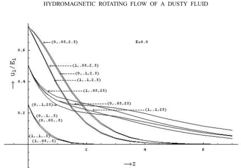
To investigate the effect of various flow parameters on the fluid velocity and the wall shear stress, the exact solutions (3.8) and (5.2) are evaluated for the cases E =0,E =0.1 andE =1.0 withT =2. These values ofEandT are taken as typical although actual values can be used according to the physical situations. The changing nature of the velocity profiles are incorporated in Figures 3, 4(a,b) and 5(a,b) for different values of the particle concentration(k), the magnetic field (n)and time. It is observed from Figure 3 that in absence of rotation(E =0) both the particles and the magnetic field produce diminishing effect on the fluid velocityu1as long as time remains small. But, at large time, a significant rise in the magnitude of the fluid velocity near the plate due to particles is noticed although the magnetic field continues to exert damping effect on it. This is a consequence of the effect of pulsation on the flow near the plate in absence of rotation.
Figure 3 – Variation of the fluid velocityu1for different values of(k,n,t)whenT =2
andE =0.0.
near the plate decreases compared to non-rotating case while theu2component of velocity which appears due to rotation increases near the plate with the increase of particle concentration(k). As a result, the fluid velocity near the plate increases with the particles only at large values of time when rotation is small. Such a phenomenon is not found when rotation is large. We therefore say that pulsation exerts its influence on the flow near the plate only when rotation is small and time is large.
Figure 4(a) – Variation of the fluid velocity componentu1for different values of(k,n,t)
whenT =2 andE =0.1.
Figure 4(b) – Variation of the fluid velocity componentu2for different values of(k,n,t)
Figure 5(a) – Variation of the fluid velocity componentu1for different values of(k,n,t)
whenT =2 andE =1.0.
Figure 5(b) – Variation of the fluid velocity componentu2for different values of(k,n,t)
A comparative study of the magnitude of the fluid velocity produced by pulsa-tion of the plate has been made with that generated by impulsively moved plate for small and large values of rotation particularly when time is large. The results are presented in Figures 6, 7(a,b) and 8(a,b). The distinctive feature of this study is that the magnitude of the fluid velocity near the plate remains always higher in an impulsively generated flow compared to its value produced by pulsation of the plate. Moreover, in presence of pulsation, the increasing effect of the particles onu1component of fluid velocity near the plate for small rotation and large time, is totally absent in a similar situation when the flow is generated by impulsively moved plate. Additionally, the effect of pulsation on the particles to increase the fluid velocity near the plate in the case of small rotation and large time can be minimized with the increase of rotation (see Table I). In all other cases, the particles and the magnetic field produce diminishing effect on the fluid velocity near the plate for both the types of motion mentioned above.
Figure 6 – Fluid velocityu1for different values of(k,n)whenT = 2, E =0.0 and
t=25 corresponding to both pulsatile and impulsive motion of the plate.
Figure 7(a) – Variation of the fluid velocity componentu1for different values of(k,n)
whenT =2,E=0.1 andt =25 corresponding to both pulsatile and impulsive motion of the plate.
Figure 7(b) – Variation of the fluid velocity componentu2for different values of(k,n)
Figure 8(a) – Variation of the fluid velocity componentu1for different values of(k,n)
whenT =2,E=1.0 andt =25 corresponding to both pulsatile and impulsive motion of the plate.
Figure 8(b) – Variation of the fluid velocity componentu2for different values of(k,n)
E t n k (|qz|,θ ) 0.0 0.5 1.0 1.5 2.0 2.5 0.1 2.5 0.05 0.0 |q| 0.750 0.642 0.488 0.339 0.220 0.135
θ 0.0 -.0324 -.0563 -.0759 -.0932 -.1089 1.0 |q| 0.750 0.568 0.383 0.237 0.137 0.075
θ 0.0 -.0331 -.0566 -.0755 -.0919 -.1066 0.1 1.0 |q| 0.750 0.561 0.374 0.229 0.131 0.071
θ 0.0 -.0327 -.0560 -.0748 -.0911 -.1058 25 0.05 0.0 |q| 0.5 0.336 0.261 0.234 0.225 0.218
θ 0.0 -.1001 -.2307 -.3494 -.4356 -.4994 1.0 |q| 0.5 0.339 0.272 0.243 0.222 0.201
θ 0.0 -.1608 -.3429 -.4940 -.6106 -.7090 0.1 1.0 |q| 0.5 0.330 0.255 0.220 0.195 0.172
θ 0.0 -.1411 -.3047 -.4440 -.5523 -.6434 1.0 2.5 0.05 0.0 |q| 0.750 0.602 0.446 0.306 0.197 0.121
θ 0.0 -.3078 -.5446 -.7431 -.9196 -1.080 1.0 |q| 0.750 0.528 0.346 0.211 0.121 0.066
θ 0.0 -.3103 -.5439 -.7355 -.9032 -1.055 0.1 1.0 |q| 0.750 0.522 0.339 0.205 0.117 0.063
θ 0.0 -.3062 -.5378 -.7283 -.8954 -1.047 25 0.05 0.0 |q| 0.5 0.248 0.114 0.077 0.083 0.084
θ 0.0 -.2770 -.7978 -1.669 -2.215 -2.451 1.0 |q| 0.5 0.208 0.083 0.060 0.057 0.047
θ 0.0 -.3188 -.9945 -1.909 -2.343 -2.530 0.1 1.0 |q| 0.5 0.208 0.082 0.057 0.053 0.044
θ 0.0 -.3118 -.9621 -1.871 -2.316 -2.603
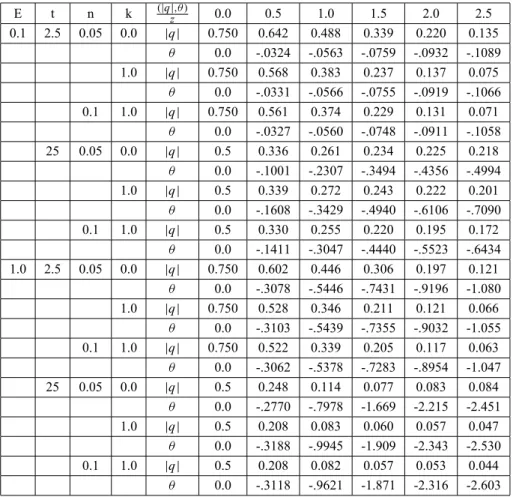
Table 1 – Magnitude|q|and inclinationθof the fluid velocity vector near the plate for different values ofE,t,n,k.
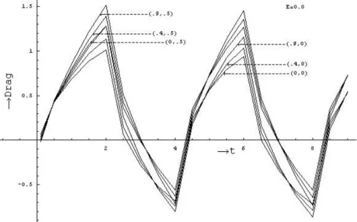
when E =0.0 and E =0.1, the maximum value of the drag is found to occur at aboutt = 2τ which for large rotation(E = 1.0)appears at about t = 6τ. Similar is the case for the appearance of the minimum value of the drag on the plate. This shows that the time of occurrence of the maximum and the minimum of the drag on the plate depends on rotation. In general, the drag on the plate is increased by rotation, the magnetic field and the particles with the effect of rotation increased due to the particles and diminished due to the magnetic field. For instance, whent =5.0,n=0.3 andEis increased from 0.1 to 1.0, the drag on the plate increases by 0.242% and 0.338% fork =0.4 and 0.9 respectively. Similarly, fort = 5.0, k = 0.4 and E is increased from 0.1 to 1.0, the drag on the plate increases by 0.242% and 0.174% forn =0.3 and 0.5 respectively. Moreover, we find that the increasing effect of the particles on the drag dimin-ishes due to increase of the magnetic field both in the rotating and non-rotating system. Finally, we notice that, for all values of rotation, the steady-state result (eqn. 5.3) contains the effect of both the particles and the magnetic field, which differs from that of impulsively moved plate, in which case, the steady-state result for the drag contains both the effects only when rotation is large [Ref. 11].
Figure 10(a) – Drag on the plate for various values of(k,n)whenT =2 andE =0.1.
Figure 10(b) – Lateral stress on the plate for various values of(k,n)whenT =2 and
E=0.1.
Figure 11(a) – Drag on the plate for various values of(k,n)whenT =2 andE =1.0.
Figure 11(b) – Lateral stress on the plate for various values of(k,n)whenT =2 and
unlike drag, the magnitude of the lateral stress diminishes with the magnetic field and increases with the particles irrespective of the values of rotation. The occurrence of the maximum value of the lateral stress depends on rotation with its minimum at the initial stage of the motion. For instance, when E = 0.1, the maximum of the lateral stress occurs at about t = 6.5τ and the same is found at about t = 2.5τ when E = 1.0. Additionally, we observe that the increasing effect of rotation on the lateral stress increases with the magnetic field and decreases with the particles which is just reversed to that observed in the case of drag on the plate.
Finally, the magnitude and inclination of the fluid velocity vector with increas-ingz and for different values of E, t,n,k are shown in the Table I so that an understanding about the propagation of disturbance away from the plate and the structure of the associated Ekman spirals can be ascertained.
7 Conclusion
The Present problem is concerned with the investigation of the unsteady motion in a fluid-particle system induced by multiple frequency unidirectional motion of the boundary instead of the motion generated by oscillations of the boundary with constant frequency about a constant mean as considered by the authors [11]. Accordingly, the flow phenomena encountered by the present authors and the au-thors [11] are not the same. In the present investigation, the velocity distribution remains unidirectional and positive for all the time instead of oscillating posi-tive and negaposi-tive flows as obtained by the authors [11]. However, the present findings coincide with those of authors [11] only in the case of an impulsively moved plate as it represents the same motion. It is further to be noted that blood flows in large arteries, some atmospheric and oceanic flows driven by pressure pulses and other similar problems associated with astrophysics, which are gen-erally considered as unidirectional pulsatile flows, may easily be investigated following the present analysis instead of that given by authors [11].
rotation, (ii) the intensity of pulsatile flow near the plate remains always less than the impulsively generated flow, (iii) the magnetic field and the particles require some time to exert their influence on the drag and the lateral stress from the beginning of the unsteady motion of the plate caused by the pulses. This is true for all values of rotation, (iv) for all values of rotation, the magnitude of drag is increased by both the magnetic field and the particles while the magnitude of the lateral stress is decreased by the magnetic field and increased by the particles.
Acknowledgement. The authors are grateful to the referees for providing many useful suggestions to improve the paper in its present form.
REFERENCES
[1] A.K. Ghosh,Flow of viscous liquid set up between two co-axial cylinders due to pulses of longitudinal impulses applied on the inner cylinder. J. Sci. Engg. Res.,9(2) (1965), 222.
[2] A. Chakraborty and J. Ray,Unsteady magnetohydrodynamic Couette flow between two plates when one of the plates is subjected to random pulses. J. Phys. Soc. Jpn.,48(1980), 1361.
[3] M.N. Makar,Magnetohydrodynamic flow between two plates when one of the plates is sujected to tooth pulses. Acta Phys. Pol.,A71(1987), 995.
[4] A.R. Bestman and F.I. Njoku, On hydromagnetic channel flow induced by tooth pulses. Preprint IC/88/10, Miramare-Trieste, (1988).
[5] N. Datta, D.C. Dalal and S.K. Misra,Unstesdy heat transfer to pulsatile flow of a dusty viscous incompressible fluid in a channel. Int. J. Heat Mass Transfer,36(7) (1993), 1783.
[6] N. Datta and D.C. Dalal,Pulsatile flow and heat transfer of a dusty fluid through an infinitely long annular pipe. Int. Multiphase Flow,21(3) (1995), 515.
[7] A.K. Ghosh and K. Sarkar,On hydromagnetic channel flow of a dusty fluid induced by tooth pulses.J. Phys. Soc. Jpn.,64(3) (1995), 3001.
[8] A.K. Ghosh and L. Debnath,On hydromagnetic pulsatile flow of a two-phase fluid. ZAMM, 76(2) (1996), 121.
[9] S. Ghosh and A.K. Ghosh,On hydrmagnetic channel flow of a particulate suspension induced by rectified sine pulses. J. Phys. Soc. Jpn.,73(6) (2004), 1506.
[10] S. Ghosh and A.K. Ghosh,On hydromagnetic flow of a two-phase fluid near a pulsating plate.Indian J. Pure. Appl. Math.,36(10) (2005), 529.
[12] A.K. Ghosh and L. Debnath,On hydrodynamic rotating flow of a two-phase fluid. ZAMM, 75(2) (1995), 156.
[13] H.P. Greenspan,The theory of rotating fluids.Camb. Univ. Press, (1969).
[14] R. Hide and P.H. Roberts,The origin of the mean geomagnetic field. In: Physics and Chemistry of the Earth, vol. 4, Pergamon Press, New York, (1961).
[15] R.H. Dieke,Internal rotation of the sun. In: L. Goldberg (Ed.). Annual Review of Astronomy and Astrophysics, vol. 8, Annual Reviews Inc. (1970).
[16] M. Kumari and G. Nath,Unsteady MHD film flow over a rotating infinite disk. Int. J. Engg. Sci.,42(2004), 1099.
[17] P.G. Saffmam,On the stability of laminar flow of a dusty gas. J. Fluid Mech.,13(1962), 120.
[18] C. Thornley,On Stokes and Rayleigh layers in a rotating system. Quart. J. Mech. and Appl. Math.,21(1968), 451.
[19] H.T. Yang and J.V. Healy,The Stokes Problems for a conducting fluid with a suspension of particles. Appl. Sci. Res.,21(1973), 387.
[20] S.I. Pai,Magnetogasdynamics and Plasma Dynamics. Prentice Hall, Inc., Englewood Cliffs, New Jersey, 1962.