ISSN 0101-8205 www.scielo.br/cam
Global convergence of a regularized factorized
quasi-Newton method for nonlinear least
squares problems
WEIJUN ZHOU† and LI ZHANG‡
College of Mathematics and Computational Science,
Changsha University of Science and Technology, Changsha 410004, China
E-mails:†[email protected] /‡[email protected]
Abstract. In this paper, we propose a regularized factorized quasi-Newton method with a new
Armijo-type line search and prove its global convergence for nonlinear least squares problems.
This convergence result is extended to the regularized BFGS and DFP methods for solving strictly
convex minimization problems. Some numerical results are presented to show efficiency of the
proposed method.
Mathematical subject classification: 90C53, 65K05.
Key words:factorized quasi-Newton method, nonlinear least squares, global convergence.
1 Introduction
The objective of this paper is to present a globally convergent factorized quasi-Newton method for the nonlinear least squares problem
min f(x)= 1
2 m
X
i=1
ri2(x)= 1 2kr(x)k
2
, x ∈ Rn. (1.1)
Herer(x) =(r1(x),∙ ∙ ∙,rm(x))T is called the residual function which is non-linear and|| ∙ ||denotes the Euclidean norm. It is easy to show that the gradient and the Hessian of f are given by
whereJ(x)is the Jacobian matrix ofr(x),
G(x)=
m
X
i=1
ri(x)∇2ri(x)
and∇2ri(x)is the Hessian matrix ofri(x).
The nonlinear least squares problem has many applications in applied areas such as data fitting and nonlinear regression in statistics. Many efficient al-gorithms have been proposed to solve this problem. The special structure of the Hessian leads to a lot of special methods which have different convergence properties for zero and nonzero residual problems [5, 6, 8, 20].
The Gauss-Newton method and the Levenberg-Marquardt method are two well-known methods which have locally quadratic convergence rate for zero residual problems [6]. However, they may converge slowly or even diverge when the problem is nonzero residual or the residual function is highly nonlinear [1]. The main reason is that both methods only use the first order information of f.
To solve nonzero residual problems more efficiently, some structured quasi-Newton methods using the second order information of f have been proposed. These methods are shown to be superlinearly convergent for both zero and nonzero residual problems [5, 8]. However, the iterative matrices of structured quasi-Newton methods are not necessarily positive definite. Therefore the search directions may not be descent directions of f when some line search is used.
To guarantee the positive definite property of the iterative matrices, some fac-torized quasi-Newton methods have been proposed [15, 16, 18, 19, 20, 21, 22], where the search direction is given by
Jk+Lk
T
Jk+Lk
d = −JkTrk,
problems. Under suitable conditions, the iterative matrices of factorized quasi-Newton methods are proved to be positive definite if the initial point is close to the solution point [20, 24].
However, all iterative matrices of factorized quasi-Newton methods may not be positive definite if the initial point is far from the solution. Therefore, the search direction may not be descent. This is a drawback of factorized quasi-Newton methods to have global convergence when the line search methods are used. Another difficulty for the global convergence is that the iterative matrices and their inverses may not be uniformly bounded. To the best of our knowledge, global convergence of factorized quasi-Newton methods has not been estab-lished.
The paper is organized as follows. In Section 2, we propose a regularized factorized quasi-Newton method which guarantees that the iterative matrix is positive definite at each step. We use a new Armijo-type line search to compute the stepsize. Under suitable conditions, we prove that the proposed method converges globally for nonlinear least squares problems. In Section 3, we extend this result to the BFGS and DFP methods for general nonlinear optimization. We show that the regularized BFGS and DFP methods converge globally for strictly convex objective functions. In Section 4, we compare the performance of the proposed method to some existing methods and present some numerical results to show efficiency of the proposed method.
2 Algorithm and global convergence
In this section, we first present the regularized factorized quasi-Newton algo-rithm and then analyze its global convergence property. The motivation of the method is that the positive definite property of the iterative matrix can be guar-anteed by the use of the Levenberg-Marquardt regularization technique. It is important for global convergence of the method to choose suitable regulariza-tion parameter and stepsize carefully. Now we give the details of the method.
Algorithm 2.1(Regularized factorized quasi-Newton method)
Step 1. Give the starting point x0 ∈ Rn, L0 ∈ Rm×n, δ, ρ ∈ (0,1),
Letk :=0.
Step 2. Computedk by solving the linear equations
Bk+μkI
d = −gk, (2.1)
where
Bk = Jk+Lk
T
Jk+Lk
, gk = JkTrk and
μk =
(
ǫ1kBkk if kBkk>max M,kgk1k
, ǫ2kgkkr otherwise.
(2.2)
HerekBkkis referred to the Frobenius norm of Bk. For simplicity, we denote
K1=△
k|kBkk>max
M, 1
kgkk
,
K2=△
k|kBkk ≤max
M, 1
kgkk
.
Step 3. (i) Ifk ∈ K2, compute stepsizeαk =max{ρ0, ρ1,∙ ∙ ∙ }such that
f xk+αkdk
≤ f xk
+δαkgkTdk. (2.3) (ii) Ifk∈ K1, we consider the following two cases.
Case (1): f(xk+dk)≤ f(xk)+δgkTdk.If f(xk+βdk) > f(xk+dk)+δβgkTdk,
set αk = 1;Otherwise, compute stepsize αk = max{β1, β2,∙ ∙ ∙ }
satisfying
f xk+βmdk
≤ f xk+βm−1dk
+δβmgkTdk. (2.4) Case (2): f(xk+dk) > f(xk)+δgkTdk.Compute stepsizeαk =max{ρ1,∙ ∙ ∙ }
such that
f xk+ρmdk
≤ f xk
+δρmgkTdk. (2.5) Step 4. Set xk+1 = xk + αkdk. Update Lk to get Bk+1 = (Jk+1 + Lk+1)T(Jk+1+Lk+1)by certain quasi-Newton formula. Letk := k+1
Remark 2.1. (i) Since the matrix Bk is positive semidefinite, the iterative matrix Bk +μkI is positive definite, which ensures that the search direction
dk is a descent direction, that is, gkTdk < 0. The choice ofμk is based on the ideas of [9, 12, 23].
(ii) The line search (2.4) is different from the standard Armijo line search (2.3) sinceβ > 1 in (2.4). This new Armijo-type line search can accept stepsize as large as possible in Case (1). The following proposition shows that it is well-defined.
Proposition 2.1. The Algorithm2.1is well-defined.
Proof. We only need to prove that the line search (2.4) terminates finitely. If it is not true, then for infinite manym, we have
f(xk+βmdk)
βm ≤
f(xk+βm−1dk)
βm +δg
T kdk.
Letm → ∞in the above inequality, then fromβ >1, f(x) ≥ 0 for allx and
f(xk +βmdk)≤ f(xk)≤ f(x0), we have
gkTdk >0,
which leads to a contradiction.
In the convergence analysis of Algorithm 2.1, we need the following assump-tion.
Assumption A.
(I) The level set= {x ∈ Rn|f(x)≤ f(x0)}is bounded.
(II) In some neighborhood N of , f is continuously differentiable and its gradient is Lipschitz continuous, namely, there exists a constant L > 0 such that
It is clear that the sequence{xk}generated by Algorithm 2.1 is contained in. Moreover, the sequence{f(xk)}is a descent sequence. Therefore it has a limit
f∗, that is,
lim
k→∞ f(xk)= f
∗. (2.7)
In addition, from Assumption A we get that there is a positive constantγ such that
kg(x)k ≤γ , ∀x ∈. (2.8) Now we give some useful lemmas for the convergence analysis of the algo-rithm.
Lemma 2.2. Let Assumption A hold. Then we have
lim k→∞αkg
T
kdk =0. (2.9)
Proof. It follows directly from (2.3), (2.4), (2.5) and (2.7).
For convenience, we denote index sets
K3= {k|α△ ksatisfies(2.4)}, K4
△
= {k|αksatisfies(2.5)}. Then we have
K1=K3∪K4.
Lemma 2.3. If k ∈ K1, then there exists a constant c1>0such that αk ≥c1
−gT kdk
kdkk2
. (2.10)
Proof. Ifk∈ K3, then from the line search (2.4), we have
f xk+αkβdk
> f xk+αkdk
+δαkβgkTdk. By the mean values theorem and (2.6), we have
f xk+αkβdk
− f xk +αkdk
≤αk(β−1)gkTdk +L
αk(β−1)
The above two inequalities implies
αk ≥c1
−gkTdk
kdkk2 wherec1= β(L1−δ)−1
(β−1)2 >0.Here we use the conditionsβ >
1
1−δ andδ∈(0,1).
Ifk ∈ K4, then from the line search (2.5), we have
f
xk+
αk
ρ dk
> f(xk)+δ
αk
ρ g
T kdk.
Therefore the inequality (2.10) also holds by using similar proof in the case
k∈ K3.The proof is then completed sinceK1= K3∪K4.
Lemma 2.4. If k ∈ K2, then there exists a constant c2>0such that αk =1, or αk ≥c2
−gT kdk
kdkk2
. (2.11)
Proof. Fork ∈ K2, ifαk 6=1, then by the line search (2.3), we also have
f
xk+
αk
ρ dk
> f(xk)+δ
αk
ρ g
T kdk.
Then the conclusion follows directly from the same argument as Lemma 2.3.
The proof of the following lemma is similar to that of Theorem 2.2.2 of [12], for completeness, we present the proof here.
Lemma 2.5. Let Assumption A hold and the sequence{xk}be generated by
Algorithm2.1. If K1is infinite, then we have
lim inf
k→∞ kgkk =0.
Proof. Ifk ∈ K1, thenμk = ǫ1kBkk.Now we setαˉk = αk/kBkkanddˉk =
kBkkdk, then we have
ˉ
We have from (2.1) that
−gkTdˉk = dkTBkdˉk+ǫ1kBkkdkTdˉk
= dkTBkdˉk+ǫ1k ˉdkk2≥ǫ1k ˉdkk2.
(2.13)
From Lemma 2.3 and (2.12), we get
ˉ
αkk ˉdkk2=αkdkTdˉk ≥c1
−gkTdk
kdkk2
dkTdˉk =c1 −gkTdˉk
. (2.14)
This inequality together with (2.13) shows that
ˉ
αk ≥c1ǫ1. (2.15)
It follows from (2.9) and (2.12) that
lim k→∞αˉkg
T
kdˉk = lim k→∞αkg
T
kdk =0. (2.16)
The inequalities (2.15), (2.16) and (2.13) imply that
lim k→∞,k∈K1
ˉ dk =0. Therefore from the above equality and (2.1) we have
lim k→∞,k∈K1
kgkk ≤ lim k→∞,k∈K1
kBkdk+μkdkk
≤ lim k→∞,k∈K1
(kBkkkdkk +ǫ1kBkkkdkk)
= lim
k→∞,k∈K1(1+ǫ1)k ˉdkk =0.
The proof is then finished.
The following theorem shows that Algorithm 2.1 is globally convergent.
Theorem 2.6. Let Assumption A hold and the sequence{xk}be generated by
Algorithm2.1, then we have
lim inf
Proof. We suppose that the conclusion of the theorem is not true. Then there exists a constantε >0 such that for anyk ≥0, it holds that
kgkk ≥ε. (2.17)
From Lemma 2.5, we only need to consider the case thatK1is finite. Therefore there existsk0>0 such that for allk >k0,μk =ǫ2kgkkr.
It follows from (2.1) and (2.17) that
−gkTdk =dkTBkdk +ǫ2kgkkrkdkk2≥ǫ2γrkdkk2. This inequality together with Lemma 2.4 and (2.9) means that
lim
k→∞kdkk =0. (2.18)
From (2.1), (2.17) and the definition ofK2, we have
|gkk = kBkdk+μkdkk ≤ kBkk +ǫ2kgkkr
kdkk
≤
max
M,1
ε
+ǫ2γr
kdkk It follows from the above inequality and (2.18) that
lim
k→∞kgkk =0,
which contradicts with (2.17). This finishes the proof.
3 Application to nonlinear optimization
In this section, we will extend the result of Section 2 to the BFGS method and the DFP method for the general nonlinear optimization problem
min f(x), x ∈ Rn, (3.1)
The BFGS method and the DFP method are two well-known quasi-Newton methods for solving (3.1). Their updated formulas are given by
BFGS formula: Bk+1= Bk−
BkskskTBk
skTBksk
+ yky
T k
ykTsk
;
DFP formula: Bk+1=
I − yks
T k
ykTsk
Bk
I −sky
T k
ykTsk
+ yky
T k
ykTsk
;
where yk = gk+1−gk, and sk = xk+1 −xk.An important property of both methods is that Bk+1can inherit the positive definiteness ofBk ifskTyk >0 [6]. If f is strictly convex or the Wolfe line search is used, thensT
k yk >0 and Bk+1
is well-defined.
During the past three decades, global convergence of the BFGS and DFP meth-ods has received growing interests. When f is convex and the exact line search is used, Powell proved that both methods converge globally [17]. When the Wolfe line search is used, Byrd et al. [3] proved the global convergence of the convex Broyden’s class except for the DFP method. Byrd and Nocedal [2] obtained global convergence of the BFGS method with the standard Armijo line search for strongly convex function. For nonconvex optimization, counterexamples in [4, 13] show that the BFGS method may not converge globally when using exact line search or the Wolfe line search.
Li and Fukushima [11] proposed a modified BFGS method which possesses global and superlinear convergence even for nonconvex functions. Zhou and Zhang [25] extended this result to the nonmonotone case. Zhou and Li [26] proposed a modified BFGS method for nonlinear monotone equations and es-tablished its global convergence. But these modified BFGS formulas destroy the affine invariability of the standard BFGS formula. To overcome this draw-back, Liu [12] proposed a regularized BFGS method and proved that this method converges globally for nonconvex functions if the Wolfe line search is used. Liu [12] also proposed a question that whether the regularized BFGS method is globally convergent for strictly convex or nonconvex functions if Armijo-type line search is used. The answer is positive.
Corollary 3.1. Let Assumption A hold. If f is strictly convex, then for the regularized BFGS and DFP methods, we havelim infk→∞kgkk =0.
4 Numerical experiments
In this section we compare the number of iterations and function evaluations per-formance of the proposed method to some existing methods such as the Gausss-Newton method for nonlinear least squares problems. The details of six methods are listed as follows.
(1) The Gauss-Newton method, denoted GN, which has the search direction given by Bkd = −gk, Bk = JkTJk. We compute the stepsize by the stan-dard Armijo line search, that is, compute stepsizeαk =max{ρ0, ρ1,∙ ∙ ∙ } satisfying
f xk +ρmdk
≤ f xk
+δρmgkTdk, (4.1) where we chooseδ =0.1, ρ =0.5.
(2) The Levenberg-Marquardt method, denoted LM, whose search direction is defined byBkd = −gk, Bk = JkTJk+μkI, μk = kgkk. The stepsize is computed by (4.1).
(3) The factorized BFGS method [20], denoted FBFGS, whose search direc-tion is given byBkd = −gk,andBk is updated by
Bk+1= Jk+1+Lk+1 T
Jk+1+Lk+1
(4.2)
where
Lk+1= Lk+
ˉ Lksk
skTBˉksk
sT
k Bˉksk
skTzk
1/2
zk− ˉBksk
!T ,
ˉ
Lk = Jk+1+Lk,
ˉ
Bk = ˉLkTLˉk,
(4) Algorithm 2.1, denoted R-FBFGS, whereBkis updated by (4.2). Here we use the following values for the parameters: δ = 0.1, ρ = 0.5, β = 2, M=104, ǫ
1=10−8,ǫ2=1 andr =1.
(5) The scaled factorized BFGS method [24], denoted SFBFGS, whose search direction is given byBkd = −gk,andBk is updated by
Bk+1= Jk+1+ kr(xk+1)kLk+1 T
Jk+1+ kr(xk+1)kLk+1
(4.3)
where
Lk+1=
kr(xk+1)k kr(xk)k
Lk+ 1
kr(xk+1)k ˉ Lksk
skTBˉksk
sT
k Bˉksk
skTzk
1/2
zk− ˉBksk
T ,
ˉ
Lk =Jk+1+
kr(xk+1)k2 kr(xk)k
Lk,
ˉ
Bk = ˉLTkLˉk,
zk = kr(xk+1)k(Jk+1−Jk)T
r(xk+1) kr(xk)k
+JkT+1Jk+1sk. The stepsize is computed by (4.1).
(6) Algorithm 2.1, denoted R-SFBFGS, where Bk is updated by (4.3). Here we use the same parameters as R-FBFGS.
All codes were written in Matlab 7.4. In our experiments, we stopped when-everkgkk<10−4or f(xk)− f(xk+1)≤10−12max(1, f(xk+1))or the number
of iterations exceeds 104. In the methods R-FBFGS and R-SFBFGS, we set
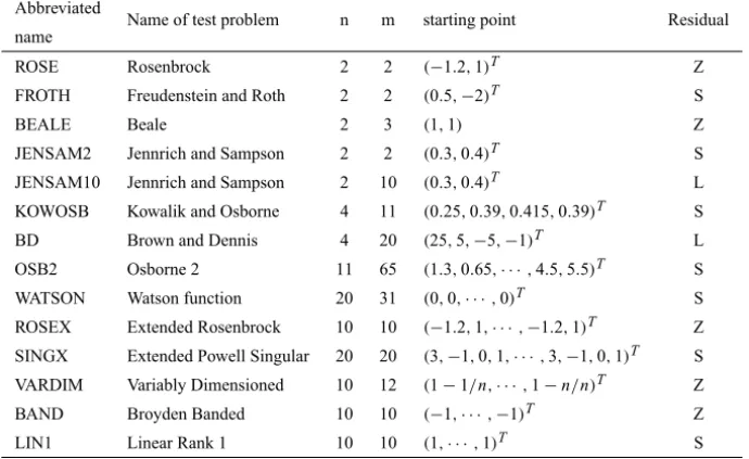
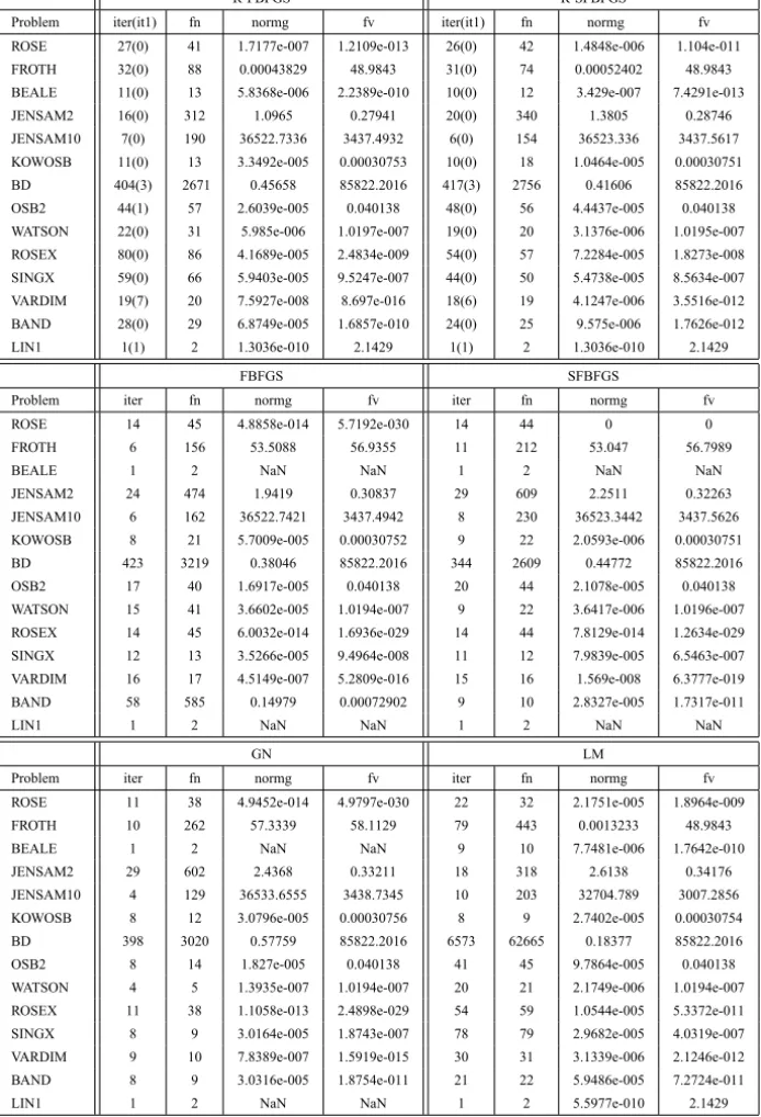
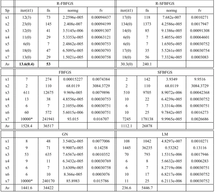
Lk+1 =0 when skTzk < 10−20. The test problems are from [14]. Table-0 lists the name and related information of the test problems, where Z, S and L stand for zero residual, small residual and large residual problems, respectively. Tables 1-4 are numerical results of these methods, where
• iter(it1) is the number of iterations(the number of iterations using the line search (2.4) for the methods R-FBFGS and R-SFBFGS);
Abbreviated
Name of test problem n m starting point Residual name
ROSE Rosenbrock 2 2 (−1.2,1)T Z
FROTH Freudenstein and Roth 2 2 (0.5,−2)T S
BEALE Beale 2 3 (1,1) Z
JENSAM2 Jennrich and Sampson 2 2 (0.3,0.4)T S JENSAM10 Jennrich and Sampson 2 10 (0.3,0.4)T L KOWOSB Kowalik and Osborne 4 11 (0.25,0.39,0.415,0.39)T S BD Brown and Dennis 4 20 (25,5,−5,−1)T L OSB2 Osborne 2 11 65 (1.3,0.65,∙ ∙ ∙,4.5,5.5)T S WATSON Watson function 20 31 (0,0,∙ ∙ ∙,0)T S ROSEX Extended Rosenbrock 10 10 (−1.2,1,∙ ∙ ∙,−1.2,1)T Z SINGX Extended Powell Singular 20 20 (3,−1,0,1,∙ ∙ ∙,3,−1,0,1)T S VARDIM Variably Dimensioned 10 12 (1−1/n,∙ ∙ ∙,1−n/n)T Z BAND Broyden Banded 10 10 (−1,∙ ∙ ∙,−1)T Z LIN1 Linear Rank 1 10 10 (1,∙ ∙ ∙,1)T S
Table 0 – Test problems.
• fv and Av stand for the functional evaluation at the stopping point and the average of corresponding measure index, respectively;
• * means that the number of iterations exceeds 104;
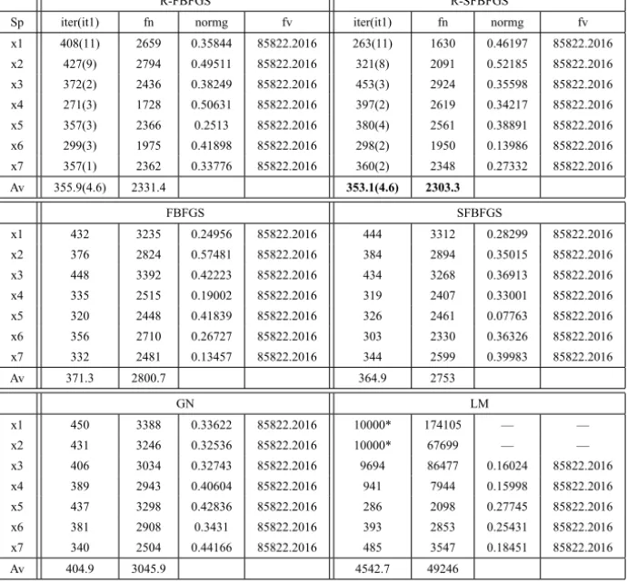
• Sp is the starting point for the problems BD, VARDIM and KOWOSB. Here we use seven different starting points, that is,x1=(103,∙ ∙ ∙ ,103)T,
x2=(102,∙ ∙ ∙,102)T, x3=(101,∙ ∙ ∙ ,101)T,x4=(1,∙ ∙ ∙,1)T,x5= (10−1,∙ ∙ ∙,10−1)T,x6=(10−2,∙ ∙ ∙,10−2)T,x7=(10−3,∙ ∙ ∙,10−3)T. As can be seen in Table 2, the method R-SFBFGS performed best for the problem BD since it requires the least number of iterations and function evalua-tions. The method R-FBFGS was faster than the methods LM and GN. Table 2 also shows that the method LM may not converge for this large residual problem since it fails to solve this problem within 104iterations when chosen the starting points x1 and x2. Tables 1 and 3 indicate that the method GN was the most efficient method for zero residual problems.
R-FBFGS R-SFBFGS
Problem iter(it1) fn normg fv iter(it1) fn normg fv
ROSE 27(0) 41 1.7177e-007 1.2109e-013 26(0) 42 1.4848e-006 1.104e-011
FROTH 32(0) 88 0.00043829 48.9843 31(0) 74 0.00052402 48.9843
BEALE 11(0) 13 5.8368e-006 2.2389e-010 10(0) 12 3.429e-007 7.4291e-013
JENSAM2 16(0) 312 1.0965 0.27941 20(0) 340 1.3805 0.28746
JENSAM10 7(0) 190 36522.7336 3437.4932 6(0) 154 36523.336 3437.5617
KOWOSB 11(0) 13 3.3492e-005 0.00030753 10(0) 18 1.0464e-005 0.00030751
BD 404(3) 2671 0.45658 85822.2016 417(3) 2756 0.41606 85822.2016
OSB2 44(1) 57 2.6039e-005 0.040138 48(0) 56 4.4437e-005 0.040138
WATSON 22(0) 31 5.985e-006 1.0197e-007 19(0) 20 3.1376e-006 1.0195e-007
ROSEX 80(0) 86 4.1689e-005 2.4834e-009 54(0) 57 7.2284e-005 1.8273e-008
SINGX 59(0) 66 5.9403e-005 9.5247e-007 44(0) 50 5.4738e-005 8.5634e-007
VARDIM 19(7) 20 7.5927e-008 8.697e-016 18(6) 19 4.1247e-006 3.5516e-012
BAND 28(0) 29 6.8749e-005 1.6857e-010 24(0) 25 9.575e-006 1.7626e-012
LIN1 1(1) 2 1.3036e-010 2.1429 1(1) 2 1.3036e-010 2.1429
FBFGS SFBFGS
Problem iter fn normg fv iter fn normg fv
ROSE 14 45 4.8858e-014 5.7192e-030 14 44 0 0
FROTH 6 156 53.5088 56.9355 11 212 53.047 56.7989
BEALE 1 2 NaN NaN 1 2 NaN NaN
JENSAM2 24 474 1.9419 0.30837 29 609 2.2511 0.32263
JENSAM10 6 162 36522.7421 3437.4942 8 230 36523.3442 3437.5626
KOWOSB 8 21 5.7009e-005 0.00030752 9 22 2.0593e-006 0.00030751
BD 423 3219 0.38046 85822.2016 344 2609 0.44772 85822.2016
OSB2 17 40 1.6917e-005 0.040138 20 44 2.1078e-005 0.040138
WATSON 15 41 3.6602e-005 1.0194e-007 9 22 3.6417e-006 1.0196e-007
ROSEX 14 45 6.0032e-014 1.6936e-029 14 44 7.8129e-014 1.2634e-029
SINGX 12 13 3.5266e-005 9.4964e-008 11 12 7.9839e-005 6.5463e-007
VARDIM 16 17 4.5149e-007 5.2809e-016 15 16 1.569e-008 6.3777e-019
BAND 58 585 0.14979 0.00072902 9 10 2.8327e-005 1.7317e-011
LIN1 1 2 NaN NaN 1 2 NaN NaN
GN LM
Problem iter fn normg fv iter fn normg fv
ROSE 11 38 4.9452e-014 4.9797e-030 22 32 2.1751e-005 1.8964e-009
FROTH 10 262 57.3339 58.1129 79 443 0.0013233 48.9843
BEALE 1 2 NaN NaN 9 10 7.7481e-006 1.7642e-010
JENSAM2 29 602 2.4368 0.33211 18 318 2.6138 0.34176
JENSAM10 4 129 36533.6555 3438.7345 10 203 32704.789 3007.2856
KOWOSB 8 12 3.0796e-005 0.00030756 8 9 2.7402e-005 0.00030754
BD 398 3020 0.57759 85822.2016 6573 62665 0.18377 85822.2016
OSB2 8 14 1.827e-005 0.040138 41 45 9.7864e-005 0.040138
WATSON 4 5 1.3935e-007 1.0194e-007 20 21 2.1749e-006 1.0194e-007
ROSEX 11 38 1.1058e-013 2.4898e-029 54 59 1.0544e-005 5.3372e-011
SINGX 8 9 3.0164e-005 1.8743e-007 78 79 2.9682e-005 4.0319e-007
VARDIM 9 10 7.8389e-007 1.5919e-015 30 31 3.1339e-006 2.1246e-012
BAND 8 9 3.0316e-005 1.8754e-011 21 22 5.9486e-005 7.2724e-011
LIN1 1 2 NaN NaN 1 2 5.5977e-010 2.1429
R-FBFGS R-SFBFGS
Sp iter(it1) fn normg fv iter(it1) fn normg fv
x1 408(11) 2659 0.35844 85822.2016 263(11) 1630 0.46197 85822.2016
x2 427(9) 2794 0.49511 85822.2016 321(8) 2091 0.52185 85822.2016
x3 372(2) 2436 0.38249 85822.2016 453(3) 2924 0.35598 85822.2016
x4 271(3) 1728 0.50631 85822.2016 397(2) 2619 0.34217 85822.2016
x5 357(3) 2366 0.2513 85822.2016 380(4) 2561 0.38891 85822.2016
x6 299(3) 1975 0.41898 85822.2016 298(2) 1950 0.13986 85822.2016
x7 357(1) 2362 0.33776 85822.2016 360(2) 2348 0.27332 85822.2016
Av 355.9(4.6) 2331.4 353.1(4.6) 2303.3
FBFGS SFBFGS
x1 432 3235 0.24956 85822.2016 444 3312 0.28299 85822.2016
x2 376 2824 0.57481 85822.2016 384 2894 0.35015 85822.2016
x3 448 3392 0.42223 85822.2016 434 3268 0.36913 85822.2016
x4 335 2515 0.19002 85822.2016 319 2407 0.33001 85822.2016
x5 320 2448 0.41839 85822.2016 326 2461 0.07763 85822.2016
x6 356 2710 0.26727 85822.2016 303 2330 0.36326 85822.2016
x7 332 2481 0.13457 85822.2016 344 2599 0.39983 85822.2016
Av 371.3 2800.7 364.9 2753
GN LM
x1 450 3388 0.33622 85822.2016 10000* 174105 — —
x2 431 3246 0.32536 85822.2016 10000* 67699 — —
x3 406 3034 0.32743 85822.2016 9694 86477 0.16024 85822.2016
x4 389 2943 0.40604 85822.2016 941 7944 0.15998 85822.2016
x5 437 3298 0.42836 85822.2016 286 2098 0.27745 85822.2016
x6 381 2908 0.3431 85822.2016 393 2853 0.25431 85822.2016
x7 340 2504 0.44166 85822.2016 485 3547 0.18451 85822.2016
Av 404.9 3045.9 4542.7 49246
Table 2 – Test results for the large residual problem BD.
stationary points for the given test problems. Moreover, we observe that the line search (2.4) was rarely used, but it is very efficient for the large residual problems.
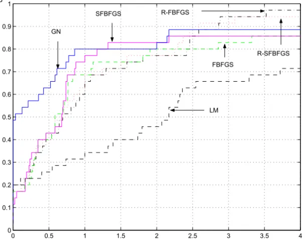
In order to show the number of iterations or function evaluations performance of the six methods more clearly, we made Figures 1-2 according to the dada in Tables 1-4 by using the performance profiles of Dolan and Moré [7].
R-FBFGS R-SFBFGS
Sp iter(it1) fn normg fv iter(it1) fn normg fv
x1 29(19) 30 7.3573e-006 1.1704e-011 34(20) 43 6.4822e-007 1.1197e-015
x2 25(16) 31 9.2223e-008 2.9985e-017 24(16) 25 1.05e-005 2.3794e-011
x3 21(12) 22 3.4701e-006 5.381e-013 21(12) 22 5.2768e-005 5.8634e-010
x4 0(0) 1 0 0 0(0) 1 0 0
x5 19(7) 20 9.4672e-007 1.7041e-013 18(7) 19 6.9588e-005 7.4793e-010
x6 20(8) 21 1.7441e-006 6.403e-014 19(7) 20 5.7122e-005 4.2315e-010
x7 20(8) 21 6.0293e-006 4.2892e-013 20(7) 21 2.4841e-008 1.3298e-016
Av 19.1(10) 20.9 19.4(9.9) 21.6
FBFGS SFBFGS
x1 29 30 5.1336e-005 6.8275e-012 30 31 4.8478e-005 6.0885e-012
x2 26 27 1.5511e-005 6.2332e-013 26 27 4.2816e-005 4.7493e-012
x3 22 23 2.3744e-007 1.4606e-016 21 22 5.1305e-005 6.8191e-012
x4 0 1 0 0 0 1 0 0
x5 17 18 2.5966e-009 1.7467e-020 16 17 1.663e-011 7.1643e-025
x6 17 18 1.1484e-007 3.4167e-017 16 17 1.2009e-008 3.7362e-019
x7 10 11 5.8861e-012 8.9756e-026 45 46 9.7049e-007 2.0374e-013
Av 17.3 18.3 22 23
GN LM
x1 20 21 1.9919e-012 1.0279e-026 10000* 10001 — —
x2 16 17 8.999e-006 2.098e-013 3152 3153 1.6329e-007 5.7681e-015
x3 13 14 7.7751e-010 1.5661e-021 302 303 5.3062e-008 6.0906e-016
x4 0 1 0 0 0 1 0 0
x5 10 11 0 0 42 43 4.3908e-008 4.1704e-016
x6 10 11 3.8833e-012 3.9067e-026 45 46 4.7351e-008 4.8502e-016
x7 10 11 5.8861e-012 8.9756e-026 45 46 9.7049e-007 2.0374e-013
Av 11.3 12.3 1940.9 1941.9
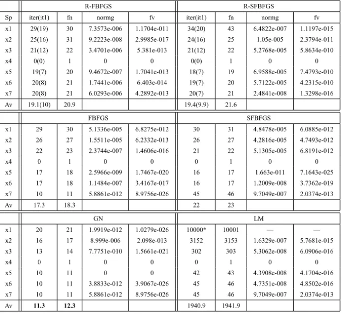
Table 3 – Test results for the zero residual problem VARDIM.
problems successfully while the methods R-FBFGS and R-SFBFG can solve all test problems. For τ > 2, the top curves correspond to R-FBFGS and R-SFBFGS, which shows that both methods are best within a factor τ with respective to the number of iterations and function evaluations.
Conclusions
R-FBFGS R-SFBFGS
Sp iter(it1) fn normg fv iter(it1) fn normg fv
x1 12(3) 73 2.2596e-005 0.00094437 17(0) 118 7.682e-007 0.0010271
x2 23(0) 145 2.408e-007 0.00094199 134(0) 1373 4.2586e-005 0.0017947
x3 12(0) 41 3.5145e-006 0.00091307 14(0) 85 9.1386e-005 0.00091308
x4 11(0) 29 5.3353e-005 0.00063121 6(0) 7 5.4055e-005 0.00064601
x5 6(0) 7 2.4862e-005 0.00030753 6(0) 7 1.6505e-005 0.00030752
x6 18(0) 47 6.5095e-005 0.00030793 17(0) 35 5.5261e-005 0.00030754
x7 13(0) 29 1.5021e-005 0.00030758 18(0) 56 7.3324e-005 0.0003083
Av 13.6(0.4) 53 30.3(0) 240.1
FBFGS SFBFGS
x1 7 274 0.00015227 0.0074384 2 142 3.9349 9.9516
x2 2 110 68.0119 3084.3729 2 110 68.0119 3084.3729
x3 611 12675 9.969e-005 0.0079896 510 9705 8.9072e-006 0.00042368
x4 13 38 4.8556e-005 0.00030753 10 22 6.4239e-005 0.00030752
x5 6 7 2.1055e-006 0.00030751 6 7 3.3314e-006 0.00030751
x6 60 572 5.6015e-006 0.00030751 10 25 9.7842e-005 0.0016273
x7 10000* 241941 93.015 0.016707 7245 178138 9.9965e-005 0.0026686
Av 1528.4 36517 1112.1 26878
GN LM
x1 8 48 3.5482e-005 0.0077006 108 1042 4.8297e-007 0.0010271
x2 9 71 9.9007e-005 0.14258 1445 36235 0.53282 0.13116
x3 53 635 7.6567e-005 0.0010352 70 793 1.5315e-006 0.0017946
x4 9 11 6.3432e-005 0.00030769 6 8 5.6632e-005 0.0006283
x5 6 7 3.6309e-005 0.00030758 6 7 8.2719e-006 0.00030751
x6 6 10 8.366e-005 0.0003076 10 17 6.8217e-006 0.00030752
x7 10000* 240170 85.8983 0.015786 11 25 6.2113e-006 0.00030752
Av 1441.6 34422 236.6 5446.7
Table 4 – Test results for the small residual problem KOWOSB.
Acknowledgement. Part work of the first author was done when he was visiting Hirosaki University. This work was partially supported by the NSF foundation (10901026) of China, a project (09B001) of Scientific Research Fund of Hunan Provincial Education Department, the Hong Kong Polytechnic University Post-doctoral Fellowship Scheme and a scholarship from the Japanese Government.
REFERENCES
[1] M. Al-Baali and R. Fletcher,Variational methods for non-linear least squares.J. Oper. Res. Soc.,36(1985), 405–421.
[2] R.H. Byrd and J. Nocedal,A tool for the analysis of quasi-Newton methods with application to unconstrained minimization. SIAM J. Numer. Anal.,26(1989), 727–739.
0 0.5 1 1.5 2 2.5 3 3.5 4 0
0.1 0.2 0.3 0.4 0.5 0.6 0.7 0.8 0.9 1 P
τ
R-FBFGS
R-SFBFGS
FBFGS SFBFGS
GN
LM
Figure 1 – Performance profiles with respect to the number of iterations.
0 0.5 1 1.5 2 2.5 3 3.5 4
0 0.1 0.2 0.3 0.4 0.5 0.6 0.7 0.8 0.9 1
R-FBFGS
R-SFBFGS
FBFGS SFBFGS
GN
LM P
τ
[4] Y.H. Dai, Convergence properties of the BFGS algorithm. SIAM J. Optim.,13(2002), 693–701.
[5] J.E. Dennis, H.J. Martínez and R.A. Tapia, Convergence theory for the structured BFGS secant method with application to nonlinear least squares.J. Optim. Theory Appl.,61(1989), 161–178.
[6] J.E. Dennis and H.J. Schnabel, Numerical methods for unconstrained optimization and nonlinear equations.Prentice-Hall, Englewood Cliffs, NJ (1983).
[7] E.D. Dolan and J.J. Moré, Benchmarking optimization software with performance profiles. Math. Program.,91(2002), 201–213.
[8] J.R. Engels and H.J. Martínez, Local and superlinear for partially known quasi-Newton methods.SIAM J. Optim.,1(1991), 42–56.
[9] J. Fan and Y. Yuan, On the quadratic convergence of the Levenberg-Marquardt method without nonsingularity assumption.Computing,74(2005), 23–39.
[10] J. Huschens,On the use of product structure in secant methods for nonlinear least squares problems.SIAM J. Optim.,4(1994), 108–129.
[11] D.H. Li and M. Fukushima, A modified BFGS method and its global convergence in nonconvex minimization.J. Comput. Appl. Math.,129(2001), 15–35.
[12] T.W. Liu, BFGS method and its application to constrained optimization. Ph.D. thesis, College of Mathematics and Econometrics, Hunan University, Changsha, China (2007).
[13] W.F. Mascarenhas,The BFGS method with exact line searches fails for non-convex objective functions.Math. Program.,99(2004), 49–61.
[14] J.J. Moré, B.S. Garbow, K.E. Hillstrom,Testing unconstrained optimization software.ACM Trans. Math. Softw.,7(1981), 17–41.
[15] H. Ogasawara, A note on the equivalence of a class of factorized Broyden families for nonlinear least squares problems.Linear Algebra Appl.,297(1999), 183–191.
[16] H. Ogasawara and H. Yabe, Superlinear convergence of the factorized structured quasi-Newton methods for nonlinear optimization.Asia-Pacific J. Oper. Res.,17(2000), 55–80.
[17] M.J.D. Powell,On the convergence of the variable metric algorithms.J. Inst. Math. Appl.,
7(1971), 21–36.
[18] C.X. Xu, X.F. Ma and M.Y. Kong, A class of factorized quasi-Newton methods for non-linear least squares problems.J. Comput. Math.,14(1996), 143–158.
[19] H. Yabe and T. Takahashi, Structured quasi-Newton methods for nonlinear least squares problems.TRU Math.,24(1988), 195–209.
[21] H. Yabe and N. Yamaki, Convergence of a factorized Broyden-like family for nonlinear least squares problems.SIAM J. Optim.,5(1995), 770–791.
[22] H. Yabe and N. Yamaki, Local and superlinear convergence of structured quasi-Newton methods for nonlinear optimization. J. Oper. Res. Soc. Japan,39(1996), 541–557.
[23] N. Yamashita and M. Fukushima,On the rate of convergence of the Levenberg-Marquardt method.Computing (Supp.),15(2001), 237–249.
[24] J.Z. Zhang, L.H. Chen and N.Y. Deng,A family of scaled factorized Broyden-like methods for nonlinear least squares problems.SIAM J. Optim.,10(2000), 1163–1179.
[25] W. Zhou and L. Zhang,Global convergence of the nonmonotone MBFGS method for non-convex unconstrained minimization. J. Comput. Appl. Math.,223(2009), 40–47.