www.the-cryosphere.net/9/2135/2015/ doi:10.5194/tc-9-2135-2015
© Author(s) 2015. CC Attribution 3.0 License.
From Doktor Kurowski’s Schneegrenze to our modern glacier
equilibrium line altitude (ELA)
R. J. Braithwaite
School of Environment, Education and Development (SEED), University of Manchester, Manchester, UK Correspondence to:R. J. Braithwaite (r.braithwaite@manchester.ac.uk)
Received: 15 May 2015 – Published in The Cryosphere Discuss.: 17 June 2015
Revised: 21 September 2015 – Accepted: 2 October 2015 – Published: 18 November 2015
Abstract. Translated into modern terminology, Kurowski suggested in 1891 that the equilibrium line altitude (ELA) of a glacier is equal to the mean altitude of the glacier when the whole glacier is in balance between accumulation and ab-lation. Kurowski’s method has been widely misunderstood, partly due to inappropriate use of statistical terminology by later workers, and has only been tested by Braithwaite and Müller in a 1980 paper (for 32 glaciers). I now compare Kurowski’s mean altitude with balanced-budget ELA cal-culated for 103 present-day glaciers with measured surface mass-balance data. Kurowski’s mean altitude is significantly higher (at 95 % level) than balanced-budget ELA for 19 out-let and 42 valley glaciers, but not significantly higher for 34 mountain glaciers. The error in Kurowski mean altitude as a predictor of balanced-budget ELA might be due to gener-ally lower balance gradients in accumulation areas compared with ablation areas for many glaciers, as suggested by sev-eral workers, but some glaciers have higher gradients, pre-sumably due to precipitation increase with altitude. The rel-atively close agreement between balanced-budget ELA and mean altitude for mountain glaciers (mean error – 8 m with standard deviation 59 m) may reflect smaller altitude ranges for these glaciers such that there is less room for effects of different balance gradients to manifest themselves.
1 Introduction
Ludwig Kurowski was born in 1866 in Napajedla, Moravia (then in the Austrian Empire and now in the Czech Republic), and died in 1912 in Vienna (http://mahren.germanistika.cz). For his doctoral-thesis research at the University of Vienna, Kurowski (1891) studied the snow line (German:
Schnee-grenze) in the Finsteraarhorn region of the Swiss Alps. He suggested the altitude of the snow line on a glacier is equal to the mean altitude of the glacier when snow accumulation and melt are in balance for the whole glacier. A relatively recent definition of snow line (Armstrong et al., 1973) is “the line or zone on land that separates areas in which fallen snow disappears in summer from areas in which snow re-mains throughout the year. The altitude of the snow line is controlled by temperature and the amount of snowfall (cf. equilibrium lineandfirn line)”. Students of snow line in the 19th century would have broadly agreed with this definition before Ratzel (1886) introduced extra terms likeclimaticand orographicto qualify snow line. Ratzel (1886) also argued that the material left at the end of the melt season isfirn rather thansnowbut Kurowski (1891) does not use Ratzel’s preferred termFirngrenze.
The snow line definition above explicitly refers to the landscape at the end of summer as being snow-covered or snow-free, but a mass-balance concept is also implicit in the definition, i.e. snowmelt equals snow accumulation at the snow line, and this is the aspect of snow line studied by Kurowski (1891).
became accepted as standard by the late 1960s (Anony-mous, 1969). The distinction between firn line and equilib-rium line is marked for high latitude glaciers, e.g. in Green-land or on Arctic isGreen-lands, but is quite unimportant for the Alpine glaciers studied by Kurowski and other pioneers. We can therefore translate Kurowski’sSchneegrenze(where snowmelt equals snow accumulation) as equilibrium line (where mass balance is zero) and regard most late 19th cen-tury snow line (a.k.a. firn line) methods as being equally ap-plicable to equilibrium line. The best review in English of models for indirect estimation of firn lines (a.k.a. equilibrium lines) is in an obscure book-chapter by Osmaston (1975), which I only discovered when preparing a late draft of the present paper.
The simple theory of Kurowski (1891) depends on the as-sumption that mass-balance gradient is constant across the whole altitude range of the glacier. This was criticized by Hess (1904) and Reid (1908), and several modern authors have attempted to account for variations in mass-balance gra-dients by defining a ratio (“balance ratio”) between balance gradients in the ablation and accumulation zones (Furbish and Andrews, 1984; Osmaston, 2005; Rea, 2009). Kurowski himself argued that non-linearity in the balance–altitude equation need not cause a large error as low and high al-titudes on a glacier usually coincide with small areas, and are not weighted heavily in calculating mean altitude. It is surprising that nobody has verified the basic Kurowski the-ory with observed mass-balance data except for Braithwaite and Müller (1980). The main purpose of the present paper is to critically test the original Kurowski (1891) theory with observed mass-balance data from more glaciers, and then to discuss the results together with balance ratio data from Rea (2009).
Readers need not share my wish to honour Kurowski’s pioneering work, involving one of the earliest quantita-tive models in glaciology, but they should agree that the estimation of glacier ELA from topographic proxies is still an active and legitimate area of research in glaciol-ogy and quaternary science. Recent ELA-related work in-cludes Benn and Lehmkuhl (2000), Kaser and Osmas-ton (2002), Cogley and McIntyre (2003), Leonard and Foun-tain (2003), Carrivick and Brewer (2004), Benn et al. (2005), Osmaston (2005), Dyurgerov et al. (2009), Braithwaite and Raper (2009), Rea (2009), Kern and László (2010), Bakke and Nesje (2011), Rabatel et al. (2013), Ignéczi and Nagy (2013) and Heymann (2014), to cite only a few. The possibilities of monitoring year-to-year variations in the end-of-summer snow line (EOSS) from aircraft (Chinn, 1995) or from satellite images (Rabatel et al., 2005, 2012; Mathieu et al., 2014) raise similar needs to estimate proxy ELAs for present-day glaciers for which there are no observed mass-balance data.
2 Tutorial on glacier altitudes
Kurowski’s work has often been ignored or misquoted, his name is sometimes wrongly spelled following Hess (1904), and Sissons (1974) and Sutherland (1984) rediscovered his method without citing him. Because of many misquotes the reader may not understand Kurowski’s method unless he/she has him/herself read the original article. A PDF of the orig-inal article (kindly provided by Hans-Dieter Schwartz of the Bavarian Academy of Sciences) is available in the online Supplement. One underlying problem is the widespread mis-use of statistical terms likemeanandmedianwhen applied to glacier altitudes (Cox, 2004). This issue is so central to a discussion of Kurowski (1891) that I give a worked exam-ple, using the area–altitude distribution of Hintereisferner in the Austrian Alps in the year 2001, to illustrate concepts; see Sect. 5 for sources of data.
The graph of the area–altitude distribution in Fig. 1a looks like a histogram (probability distribution function) of alti-tudes on Hintereisferner and could have been obtained from a digital elevation model, witharearepresenting the number of pixels of equal area in each altitude interval. The mean altitude for such a distribution is
¯
h=Hmean= i=N X
i=1
hi×ai
! ,i=N X
i=1
ai, (1)
whereaiis the area of theith altitude band andhi is its alti-tude andN is the number of altitude bands. For the given
altitude–area distribution (Fig. 1a) for Hintereisferner, the mean altitudeHmeanis 3038 m a.s.l. This is the mean altitude of the glacier according to the Kurowski (1891) method and it is obvious from his Table III that he calculates his “Mittlere Höhe des Gletschers” from the altitude–area distribution of each glacier according to Eq. (1).
Some authors incorrectly assert that Kurowski (1891) used an accumulation–area ratio (AAR) of 50 % to locate the snow line (Müller, 1980; Kotlyakov and Krenke, 1982), and the guidelines of the World Glacier Inventory (TTS, 1977) in-correctly refer to this altitude as “mean altitude”. Figure 1b shows the percentage of the area lying above any particu-lar altitude (cumulative distribution function). The median altitude is that altitude dividing the glacier area into equal halves, i.e. it is the altitude (x-coordinate) corresponding to
ay-coordinate of 50 %. For the given altitude–area
distribu-tion (Fig. 1b), the median altitudeH50is 3056 m a.s.l. This is the altitude giving AAR=50 %. In a similar way, the altitude
H60above which 60 % of the glacier area lies is 2989 m a.s.l. Kurowski (1891) quotes Brückner (1886) as saying that 75 % of the glacier lies above the snow line (which nobody would believe today), andH75=2878 m a.s.l. in the present case.
Figure 1. Area–altitude distribution for Hintereisferner, Austrian Alps, for the year 2001:(a)shows areas of altitude bands vs. their mean altitudes;(b)shows percentage of glacier area above any par-ticular altitude.
the glacier are 2400 and 3727 m a.s.l respectively, and the mid-range altitude of the glacier is
Hmid =(Hmax+Hmin)2 (2)
In the present case, the mid-range altitude (Hmid) is 3064 m a.s.l.
Manley (1959) estimated ELA (or snow line or firn line) as mid-range altitude according to (2) but many authors in-correctly assert that he used the “median” altitude although Manley does not even mention the word. Authors incor-rectly using “median” for this mid-range altitude include Porter (1975), Meierding (1982), Hawkins (1985), Benn and Lehmkuhl (2000), Carrivick and Brewer (2004), Benn et al. (2005), Osmaston (2005), Rea (2009), Dobhal (2011), and Bakke and Nesje (2011) to mention only a few. Incor-rect use of terminology can be inferred in any book or paper that refers to both “median altitude” and to “AAR” without noting that the correctly defined median altitude is identical
to the altitude with AAR=50 %, e.g. Nesje and Dahl (2000), and Benn and Evans (2010).
Kurowski’s theory was purely in terms of mean altitude, correctly defined in (1), but median and mid-range alti-tudes for glaciers are generally close to the mean altitude and would be identical to it if the area–altitude distribution were symmetric. The area–altitude distribution of Hintereis-ferner (Fig. 1a) is only slightly asymmetric, being somewhat skewed to higher altitudes, but a wide variety can be found for other glaciers and it is important not to conflate the vari-ous altitudes.
3 Snow line before Kurowski
The scientific concept of snow line was discovered by the French geophysicist Pierre Bouguer (1698–1758) on an ex-pedition to tropical South America (Klengel, 1889). Up to the early 19th century, the snow line had been observed in many areas so that Alexander von Humboldt (1769–1859) could start to compile a global picture of snow line varia-tions. A version of von Humboldt’s snow line table is given in English by Kaemtz (1845, pp. 228–229) with snow line altitudes for 34 regions from all over the world. Heim (1885, pp. 18–21) gives a greatly extended table, and Hess (1904, map 1) plots a world map of glacier cover and snow line. Paschinger (1912) makes the first climatological analysis of snow line in various climatic regions.
Most of these snow line data were based on observations of an apparently sharp delineation between snow-covered and snow-free areas as seen from a distance of a few kilome-tres, typically by an observer in a valley or on a mountain pass, looking upwards into the high mountains. It was known very early that the snow line fluctuates with season, and from one year to the next, with large local spatial variations due to topography and aspect, and that the apparent sharp delin-eation between snow-covered and snow-free landscape dis-appears on closer examination to be replaced by a broad zone of snow patches, slowly morphing into a continuous snow cover (Mousson, 1854, p. 3; Heim, 1885, pp. 9–21; Ratzel, 1886; Klengel, 1889; Kurowski, 1891, p. 120). To overcome these problems, snow line has sometimes been defined as the boundary between > 50 % snow cover and < 50 % snow cover on a flat surface (Escher, 1970). All of these problems can be overcome with modern technology of regular remote sens-ing and image processsens-ing (Tang et al., 2014; Gafurov et al., 2015) but would have been nearly impossible with 19th cen-tury methods. In this sense, much of the early work on the snow line as a measure of snow-covered landscape was pre-mature.
mea-sure at the time. More fruitfully, a number of 19th century workers recognized that glacier accumulation areas occupy most of the region above the snow line so that the year-on-year accumulation of snow is offset by ice flow to lower ele-vations. More attention was then focussed on glaciers which were then being mapped in some detail for the first time in the Alps. One of the resulting map-based methods to deter-mine glacier snow line was by Kurowski (1891).
4 Kurowski’s work
Kurowski (1891) developed a simple theory for the altitude of snow line on a glacier, which may be one of the first the-ories in glaciology. I translate his theory into modern mass-balance terminology (Anonymous, 1969; Cogley et al., 2011) in the present paper although we must remember that glacier mass balance in its modern sense was not measured in the 19th century. In essence, Kurowski (1891) assumed that spe-cific mass balance bi at any altitude is proportional to the height above or below the ELA0for which the whole glacier is in balance:
bi =k×(hi−ELA0) , (3)
wherekis balance gradient on the glacier (assumed constant for the whole elevation range of the glacier) and ELA0 is the balanced-budget ELA. Some people use the term steady-state to qualify this ELA but this implies zero change in a multitude of factors rather than just the mass balance; see comments by M. F. Meier in the discussion following the papers by Braithwaite and Müller (1980) and Radok (1980), and see also Cogley et al. (2011). I have a similar objection to the term steady-state AAR used by some authors (Kern and László, 2010; Ignéczi and Nagy, 2013) and would prefer the termequilibriumAAR of Dyurgerov et al. (2009) if not balanced-budgetAAR.
Using modern terminology (Anonymous, 1969; Cogley et al., 2011), the mean specific balanceb¯of the whole glacier is the area-weighted sum of specific balances:
¯
b= i=N X
i=1
ai×bi
! ,i=N X
i=1
ai. (4)
Area-weighted averaging of both sides of (3) gives ¯
b= k× ¯h
−(k×ELA0) , (5)
whereh¯is the mean altitude of the glacier, defined by Equa-tion (1). Rearranging (5) and noting that b¯=zero (by as-sumption) gives
ELA0= ¯h=Hmean. (6)
Equation (6) expresses the identity between balanced-budget ELA and the mean altitude of the glacier. Kurowski himself
did not assume constant balance gradient casually but dis-cussed available evidence (Kurowski, 1891, pp. 126–130), including application of an early version of the degree-day model, to justify a nearly constant balance gradient. Re-markably, Kurowski (1891, p. 127) suggested a value of 0.0056 m w.e. m−1for vertical balance gradient, which is not greatly out of line with modern results for Alpine glaciers (Rabatel et al., 2005). He also tested a balance gradient pro-portional to the square root of altitude (p. 130) and suggested that it does not greatly affect the calculated ELA because of the relatively small proportions of glacier area at the low-est and highlow-est elevations. Osmaston (2005) appears to mis-understand this as he says the “AA method” (his name for Kurowski’s method) is based “on the principle of weighting the mass balance in areas far above or below the ELA by more than in those close to it”.
Kurowski (1891) presents his main results in Table III (pp. 142–147) of his paper. The data consist of measured areas for altitude bands of 150 m height from 1050 to 4200 m a.s.l. for 72 glaciers and 27 snow patches (German:Schneefleck) in the Finsteraarhorn Group, Switzerland. The work involved planimetric measurements of 744 individual area-elements, covering a total glacierized area of 461.19 km2. The small-est snow patch was 0.04 km2 and the largest glacier was 115.1 km2(Gr. Aletschgletscher). Unfortunately, there is no map showing delineations of separate glacial elements, and we would have to guess which areas were included for which glaciers if we wanted to replicate Kurowski’s work (this is beyond the scope of the present paper). According to the WGMS website (http://www.wgms.ch/products_fog/), the area of the presently delineatedGr. Aletschgletscheris much smaller than given by Kurowski, i.e. only 83.02 km2. This smaller area reflects: (1) a real reduction in glacier area since Kurowski’s time; (2) possible separation of the object seen by Kurowski into two or more objects on modern maps, either due to glacier shrinkage or to better map resolution; (3) possible overestimation of glacier-covered areas at higher al-titudes due to the oblique angle of observation by the 19th century surveyors. Effects (1) and (2) are well documented for the Alps (Abermann et al., 2009; Fischer, et al., 2014).
After so much tedious work with the planimeter, Kurowski must have been frustrated that he had no easy way of veri-fying/validating his snow line results. From Kurowski’s Ta-ble III, I can calculate the average altitude for all 99 glaciers and snow patches as 2867 m a.s.l. with a standard deviation of±181 m a.s.l., and there is a large range between minimum and maximum altitudes of 2470 and 3211 m a.s.l. for indi-vidual glaciers/snow patches. This variability within a single mountain group is in contrast to Heim (1885, pp. 18–21), where the snow line in the Central Alps of Switzerland is represented by the narrow range 2750–2800 m a.s.l., but is consistent with modern results (Rabatel et al., 2013).
and SW aspect have intermediate altitudes, and glaciers with SE, S, and W aspect have higher altitudes. Modern studies of the effect of aspect on glacier altitudes (Evans, 1977, 2006; Rabatel et al., 2013) broadly confirm the importance of as-pect claimed by Kurowski (1891).
The late 19th century work on glacier snow line by Kurowski and other workers appeared to be so successful that Hess (1904, p. 68) stated simply that snow line can be determined from maps of glacier regions rather than by di-rect observation of snow line in nature.
5 Mass balance and equilibrium line altitude
For present purposes, the most important development in 20th century glaciology was the systematic measurement of surface mass balance on selected glaciers. This involves mea-suring the mass balance at many points on the glacier surface using stakes and snow pits, and then averaging the results over the whole glacier area. The first continuing, multi-year series was started in 1946 on Storglaciären in northern Swe-den (Schytt, 1981) and surface mass-balance measurements have gradually extended to several hundred glaciers in all parts of the world (Haeberli et al., 2007). The bulk of these surface mass-balance data, including ELA and AAR data and various metadata, have been published in the five-yearly series “Fluctuations of Glaciers” (http://wgms.ch/products_ fog) and the less detailed two-yearly series “Mass Balance Bulletin” (http://wgms.ch/products_gmbb) from the World Glacier Monitoring Service. Jania and Hagen (1996), Dyurg-erov (2002), and DyurgDyurg-erov and Meier (2005) have published some additional data to those reported in WGMS publica-tions.
I have maintained my own database for surface mass bal-ance since the mid-1990s, consisting of a large data file com-piled from the above sources and a FORTRAN program to calculate statistics for the longer series (Braithwaite, 2002, 2009). Updating and correction of data in 2012–2013 in-volved checking the database against the latest version of the WGMS data (http://wgms.ch/products_gmbb). I now have surface mass-balance data for 371 glaciers, i.e. with≥1 year of mass-balance data, for the period 1946–2010. This fig-ure is volatile as new data can be expected, and the database will be updated as necessary. Of these 371 glaciers, there are some glaciers that do not appear to be in the WGMS database. This includes data published in the first two vol-umes of Fluctuations and Glaciers (in hard copy) that were never transferred to WGMS’s digital database.
As mass-balance data became available from an increasing number of glaciers, several workers (Liestøl, 1967; Hoinkes, 1970; Østrem, 1975; Braithwaite and Müller, 1980; Young, 1981; Schytt, 1981) established empirical equations linking the ELAt, in the yeart, to the mean specific balanceb¯
t in the same year:
ELAt=α+ β× ¯bt, (7)
whereαis the intercept andßis the slope of the equation. By definition, the balanced-budget ELA0=α. We can therefore calculate balanced-budget ELA0from mass-balance data, us-ing Eq. (7) as a regression equation as long as we have a few years of parallel data for surface mass balance and ELA to calibrate αandβ. In the absence of long data se-ries, Østrem and Liestøl (1961) calculated balanced-budget ELA for a number of glaciers using a balance–altitude curve from a single year of mass-balance observations. The two-yearly Glacier Mass Balance Bulletin published by WGMS (http://wgms.ch/products_gmbb) since 1988 lists balanced-budget ELA and AAR statistics for a steadily increasing number of glaciers, i.e. 29 glaciers in the 1988–1989 bulletin to 77 glaciers in the 2008–2009 bulletin. The selection crite-rion in the WGMS reports (http://wgms.ch/products_gmbb) seems to beN≥6 of record.
ELA varies greatly from year to year on any glacier. Fig-ure 2 illustrates ELA variations on Hintereisferner as an ex-ample. This large year-to-year variation, with a standard de-viation of±129 m for Hintereisferner, means that at least a few years of ELA measurement are needed to calculate a re-liable mean ELA. The mean ELA for the 55 years of record in Fig. 2 is 3037 m a.s.l. This mean ELA is slightly biased as a climatological index because it excludes the 3 years (warmest years?) when the ELA was above the maximum altitude of the glacier.
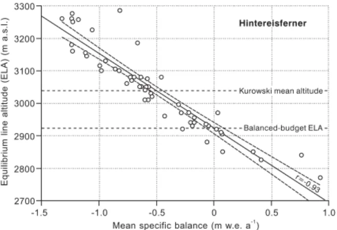
There is an obvious multi-decadal variation in ELA for Hintereisferner with a slight downward trend until the late 1970s followed by a rising trend up to the year 2010, with an increasing number of single years with ELA above the maximum altitude of the glacier. The mean ELA for the whole record (3037 m a.s.l.) is therefore too high to repre-sent the first 3 decades and too low to reprerepre-sent the last 3 decades. The mean ELA does not itself say much about the overall “health” of the glacier over the nearly 6 decades of record. A more meaningful index is the deviation of ELA from the balanced-budget ELA, i.e. the ELA needed to keep the glacier (with its current area distribution) in an overall condition of zero mass balance. The latter concept is illus-trated in Fig. 3 for Hintereisferner where yearly values of ELA are plotted against mean specific balance.
Figure 3 shows a strong negative correlation between ELA and mass balance for Hintereisferner (correlation coefficient
Figure 2.Year-to-year variations in equilibrium line altitude (ELA) at Hintereisferner, Austrian Alps, as measured in a surface mass-balance programme for 1953–2010. Gaps in the record after 2000 refer to years where ELA was above the maximum altitude of the glacier.
Figure 3.Equilibrium line altitude (ELA) plotted against mean spe-cific mass balance of Hintereisferner, Austrian Alps. Dashed lines denote 95 % confidence interval around the regression line accord-ing to Student’st-statistic.
never lower after 1980, suggesting that the present altitude– area distribution of Hintereisferner is increasingly out of equilibrium with climate.
Values of the various altitude concepts for Hintereis-ferner, discussed in Sect. 2 or above, are summarized in Ta-ble 1, clearly showing that they are clustered near the mid-dle reaches of the glacier, i.e. around 3050 m a.s.l., while balanced-budget ELA is somewhat lower. The clustering of the topographic parameters will occur for any other glacier that is somehow “fat in the middle”, although topographic “anomalies” can occur for other glaciers.
Of the total of 371 glaciers in my database with≥1 year of mass-balance data, there are 137 glaciers (37 % of total) with no ELA data (N=0), either because ELA measure-ments are not part of the observation programme or because ELA was above the glacier (ELA≥hmax)for the whole pe-riod of record. There are a further 84 glaciers (23 % of
to-Table 1.Summary of glacier altitudes for Hintereisferner, Austrian Alps, based on area–altitude data for the year 2001.
Concept Symbol Altitude
(m a.s.l.)
Mid-range altitude Hmid 3064 Median (50 %) altitude H50 3056 Kurowski mean altitude
(area-weighted mean)
Hmean 3038
Mean ELA for 1953–2010 ELA 3037 Balance-budget ELA
(intercept in ELA–balance regression equation)
ELA0 2923
tal) with less than 5 years of record for both ELA and bal-ance (5 >N≥1). This means that data from only 150 glaciers (40 % of total) are potentially available to calculate balanced-budget ELA if we regard N≥5 as sufficient for calculat-ing reliable statistics (reduced to 85 glaciers if we use the stricter criterionN≥10 years). For these 150 glaciers with the necessary data, there are generally high correlations be-tween ELA and mass balance (Fig. 4). For example, there are 143 glaciers with “good correlations” (correlation coefficient
r≤ −0.71), i.e. where the dependent variable “explains” at least half the variance of the independent variable. There are, however, seven glaciers with “poor correlations” (r>−0.7).
For a correlation coefficient approaching zero, the slope of the regression equation will also approach zero as both slope and correlation coefficient depend on the covariance of mass balance and ELA. As the slope of the regression equation approaches zero, the intercept approaches the mean of the ELA. Although low correlations between mass balance and ELA should cause errors, I did not exclude results for these seven glaciers from further analysis because I wanted to see their possible effects on final results (discussed in Sect. 6).
Rea (2009) calculated balanced-budget ELA for 66 glaciers but only includes glaciers with at least 7 years of record (N≥7) up to 2003, and excludes very small glaciers (< 1 km2). The agreements between my estimates of balanced-budget ELA and his are very close for the 66 glaciers common to both studies, i.e. with mean and standard deviation of+3 m and±25 m for the differences between the two studies.
bal-Figure 4.Histogram showing number of glaciers vs. correlation co-efficients between equilibrium line altitude (ELA) and mean spe-cific balance. The bold line denotes a Gaussian curve with the same mean and standard deviation as the plotted data.
ance of a glacier fed by frequent avalanches onto the accu-mulation area, so the available data are biased against this type of glacier. The available data cannot therefore be com-pletely representative of conditions in the real world where debris cover, calving, and substantial accumulation by snow avalanching are common, especially in the high mountain en-vironments of Benn and Lehmkuhl (2000).
6 Balanced-budget ELA and Kurowski mean altitude
Liestøl (1967) calculated balanced-budget ELA by regres-sion of ELA on measured mass balance and compared it with mean altitude for one glacier (Storbreen, Norway), and Braithwaite and Müller (1980) did the same for 32 glaciers in different parts of the world.
According to Sect. 5, balanced-budget ELAs are avail-able for 150 glaciers in the 371-glacier data set and the Kurowski mean altitude should be estimated for as many of these glaciers as possible. Detailed area–altitude data were identified in the published metadata for 148 out of the 371 glaciers. For most of these glaciers, area–altitude tables are given for every year of record (together with mass bal-ance as a function of altitude) and area–altitude data for 2001 were selected, if available, for the calculation of Kurowski mean altitude. Otherwise, data for the year closest to 2001 were selected. For a few glaciers, the area–altitude distri-bution is very out of date but nothing better is available. For Hintereisferner, the Kurowski mean altitude varies from 3010 m a.s.l. in 1965 to 3038 m a.s.l. in 2001 so errors of sev-eral decametres can occur if there is a large time difference between area–altitude and mass-balance data.
When combining the data sets for ELA0 (150 out of 371 glaciers) and Kurowski mean altitude Hmean (148 out of 371 glaciers), it was found that many glaciers had one kind of data and not the other kind, so there are in total only
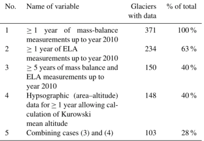
Table 2.Available surface mass-balance data for the present anal-ysis from WGMS (www.wgms.ch/products_fog.html) and some other sources.
No. Name of variable Glaciers % of total with data
1 ≥1 year of mass-balance measurements up to year 2010
371 100 %
2 ≥1 year of ELA
measurements up to year 2010
234 63 %
3 ≥5 years of mass balance and ELA measurements up to year 2010
150 40 %
4 Hypsographic (area–altitude) data for≥1 year allowing cal-culation of Kurowski mean altitude
148 40 %
5 Combining cases (3) and (4) 103 28 %
103 glaciers with data for both ELA0andHmean, Of these 103 glaciers there are now only three with poor correlations (r>−0.71).
The data availability is summarized in Table 2. It is sad to see how easily 371 glaciers with some mass-balance data have been reduced to only 103 glaciers (28 % of total) with all the information that we need for the present study. There is little that can be done about the shortness of most sur-face mass-balance series as such work is generally not well funded or resourced with the honourable exceptions of some studies in the Alps and in Scandinavia. However, the lack of published area–altitude data for some glaciers is less excus-able as such data are almost certainly availexcus-able to the data collectors. I hope that my paper will encourage workers to publish their missing area–altitude data although third par-ties could probably obtain this data using available glacier outlines from satellite images and digital elevation models. With more area–altitude data, the number of glaciers in the study could be increased to 40 % of the total. Even the sin-gle digits for “primary classification” and “frontal charac-teristics” are not available for all observed glaciers (http: //wgms.ch/products_fog).
The most obvious way of comparing balanced-budget ELA and Kurowski mean altitude is to plot anX–Y
Figure 5.Balanced-budget ELA vs. Kurowski’s mean altitude for 103 glaciers.
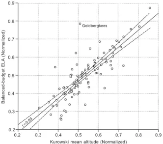
the altitude range of the glaciers before re-plotting (Fig. 6). The normalization involves subtraction of Hmin from each variable and then division by(Hmax−Hmin). The correlations between balanced-budget ELA0and Kurowski mean altitude in normalized form (Fig. 6) is lower than in Fig. 5 but is still high enough to show a satisfactory agreement (r= +0.83 for 103 glaciers) between the two variables. The regression line in Fig. 6, with its 95 % confidence interval, is slightly lower than the 1:1 line expected for ELA0=Hmean. How-ever, Cox (2004) points out that plots like Fig. 6 may also be misleading because it is the absolute difference (in me-tres) between the balanced-budget ELA and Kurowski mean altitude that we wish to see. It is convenient to define a new variable:
Emean=ELA0−Hmean, (8)
where Emean is the error in estimating ELA0 from the Kurowski mean altitudeHmean. Similar errors could be de-fined for other ways of estimating ELA0, e.g. the errorE50 usingH50orEmidusingHmidbut this is beyond the scope of the present paper.
The error ELAmean for each glacier has little relation to the correlation between ELA and balance referred to in Sect. 5, thus justifying the inclusion of several glaciers with poor ELA–balance correlations. The three glaciers with poor ELA–balance correlations (r>−0.71) have small values for errorHmean, and the glaciers with largest (+ive) difference (Goldbegkees) and smallest (−ive) difference (Bench) both have good ELA–balance correlations.
The errorEmeanis plotted in the histogram in Fig. 7. Dif-ferences of between+212 and−195 m occur but overall the differences have mean−36 m and standard deviation±56 m, indicating general agreement within a few decametres. The distribution is somewhat skewed with more negative
val-Figure 6.Balanced-budget ELA vs. Kurowski’s mean altitude for 103 glaciers with both variables normalized to the altitude range of the glaciers. The normalization of each variable involves subtrac-tion ofHminand division by(Hmax–Hmin). Dashed lines denote 95 % confidence interval around the regression line according to Student’st-statistic.
Figure 7.Histogram of errors between balanced-budget ELA and Kurowski mean altitude for 103 glaciers. The bold line denotes a Gaussian curve with the same mean and standard deviation as the plotted data.
ues than positive values so that extremely negative values in Fig. 7 are perhaps not so noteworthy. The very high posi-tive value in Fig. 7 (for Goldbergkees in the Austrian Alps) is isolated and can therefore be regarded as an “anomaly”. Braithwaite and Müller (1980) found a mean and standard deviation of−40±40 m for the differences for 32 glaciers, not including Goldbergkees as there were then no data from that glacier, which is not very different from present results.
Table 3.Mean and standard deviations of Kurowski errorEmeanfor glaciers in various regions.
Glaciers Mean SD (m a.s.l.) (m a.s.l.)
High latitudes 8 −52 ±41
Mainland N. America 19 −63 ±62
Scandinavia 29 −16 ±29
Alps 22 −16 ±71
Asia 18 −54 ±45
Tropics 5 −54 ±86
Other 2 – –
Full data set 103 −36 ±56
be expected, on Himalayan glaciers, and on glaciers in tropi-cal South America. The data for the 103 glaciers were resam-pled into seven subsets roughly representing different regions (Table 3). The high latitudes data set (eight glaciers) are from islands in the North American and Eurasian Arctic plus Mc-Call Glacier in the Brooks Range, where one would expect significant superimposed ice. The Asia data set (18 glaciers) includes glaciers from various ranges, including the Cauca-sus, but with no data from the Himalaya because there is no glacier with the necessary 5 years of ELA–balance to be included in this study. The tropics data set (5) includes four glaciers from tropical South America and one from east Africa. The overall pattern in Table 3 is for a low range of variations between groups and within groups, indicating sim-ilar performance of the Kurowski mean altitude for the dif-ferent region. The Scandinavia group has smallest errors for both mean and standard deviation, indicating the region with best performance of the Kurowski model.
One might expect the Kurowski mean altitude Hmean to perform differently for glaciers of differing morphology. This is tested with the box plot in Fig. 8 where mean and 95 % confidence intervals for the error Emean are plotted against primary classification of the glaciers using metadata from the World Glacier Monitoring website (http://wgms.ch/ products_fog/). According to the definitions in TTS (1977) the digits and their definitions are as follows: 3 Ice cap repre-sents dome-shaped ice mass with radial flow; 4 Outlet glacier drains an ice-field or ice cap, usually of valley glacier form – the catchment area may not be clearly delineated; 5 Val-ley glacier flows down a valVal-ley – the catchment area is in most cases well defined; and 6 Mountain glacier represents any shape, sometimes similar to a valley glacier but much smaller, frequently located in a cirque or niche.
Primary classification is missing for four out of the 103 glaciers. It is difficult to draw any conclusions for ice caps as there are only four cases and the confidence inter-val is very large (and unreliable). For the other morpholo-gies, it is clear that the Kurowski mean altitude significantly overestimates (at 95 % level) the balanced-budget ELA0for outlet glaciers (mean and standard deviation of −40 and
Figure 8.Box plot of mean balanced-budget ELA minus Kurowski mean altitude (ELA0–Hmean)vs. primary classification of glaciers. Error bars represent 95 % confidence intervals of the means accord-ing to Student’st-statistic. Number of glaciers in each group are given in the lower part of the diagram.
±42 m for 19 glaciers) and for valley glaciers (−50±52 m for 42 glaciers). However, for mountain glaciers the overes-timation is insignificant with a mean and standard deviation of−8±59 m for 34 glaciers.
Errors found here for Kurowski’s mean altitude may be tolerable for some applications, e.g. reconstructions of tem-perature and precipitation from traces of former glaciers (Hughes and Braithwaite, 2008). In this case, one could sim-ply calculate the Kurowski mean altitude for a reconstruction of the former glacier’s topography and then apply the appro-priate “correction” according to the primary classification of the glacier. For a “standard” vertical lapse rate of temper-ature (−0.006 K m−1) and an error of ±50 m a.s.l. in esti-mated ELA, the resulting error in estimating summer mean temperature would only be of the order±0.3 K. This is fairly small compared with the uncertainties in the relation between accumulation and summer mean temperature at the ELA re-ported by several workers: see Braithwaite (2008) for refer-ences to such studies going back to 1924.
7 Discussion
If we return to Kurowski’s theoretical treatment, his only real assumption is that balance gradient is constant over the whole glacier. It has long been supposed that this is not exactly cor-rect (Hess, 1904; Reid, 1908; Lliboutry, 1974; Braithwaite and Müller, 1980; Kuhn, 1984; Furbish and Andrews, 1984; Kaser, 2001) although Kurowski (1891) assessed the possi-ble error as small. Osmaston (2005) and Rea (2009) extend the Kurowski method to account for different balance gradi-ents but do not assess the error in the original Kurowski mean altitude.
db dh
glacier=Constant. (9)
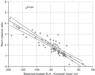
In a recent modification of the theory (Osmaston, 2005; Rea, 2009) balance gradients are different for ablation and accu-mulation areas, as expressed by the balance ratio (BR), where BR=(db/dh)abl(db/dh)acc. (10) According to Rea (2009), balance ratio greater than unity would lower the theoretical ELA, i.e. make the errorEmean negative, and balance ratio less than unity would make the er-ror positive. For the present data set, the erer-ror is negative for 84 glaciers (82 % of 103 glaciers) and positive for 19 glaciers (18 %), suggesting that balance ratio BR is commonly greater than unity but not always. Rea (2009) calculates balance ra-tio for 66 glaciers using published data for observed surface mass balance vs. altitude, and I can compare his balance ra-tios with the Kurowski errorEmean. There is a strong corre-lation (Fig. 9) between Rea’s balance ratio and the Kurowski error, i.e. r= −0.83. The very high balance ratio (BR > 5) in Fig. 9 for Zongo Glacier is an obvious anomaly although there may be good grounds to expect a reasonably large BR for tropical glaciers like this one (Kaser, 2001; Sicart et al., 2011; Rabatel et al., 2012), and the regression line in Fig. 9 does suggest a BR value a little greater than 3 for Zongo. I took the BR value for Zongo from Table 3 in Rea’s paper but in a footnote to the table referring to this point and others he notes that it “indicates a glacier where either, or both, the net balance accumulation or ablation gradient is not approx-imated by a linear relationship. AABRs for these glaciers should be treated with caution. These glaciers were not used to calculate the global AABR”. Soruco et al. (2009) report a significant revision of data from Zongo Glacier but this would have been too late for the Rea (2009) analysis. Fig-ure 9 validates the reluctance of Rea (2009) to use Zongo data in his global AABR.
This strong correlation in Fig. 9 supports the validity of the balance ratio approach. However, it is clear that the 66 glaciers in Fig. 9 show a lower proportion of glaciers with positive Kurowski error than the full data set of 103 glaciers. The box plot in Fig. 10 shows means and 95 % confi-dence intervals of Rea’s balance ratio for different types of glaciers. The solid dots refer to results from the origi-nal data (66 glaciers) of Rea (2009), while the open circles refer to an “augmented” data set (103 glaciers) where bal-ance ratios for the 37 excluded glaciers are estimated from the regression equation in Fig. 9. Leaving aside the unspec-ified and ice cap classes for which there are too few data, the plots show higher balance ratios for outlet glaciers and valley glaciers (not significantly different from BR=2 with 95 % confidence), and lower balance ratios (not significantly different from BR=1) for mountain glaciers. The increased sample size using the regression equation has doubled the number of mountain glaciers from 17 in the original data to
Figure 9.Balance ratio (Rea, 2009) plotted against Kurowski er-ror (ELA0–Hmean)for 66 glaciers. Dashed lines denote 95 % con-fidence interval around the regression line according to Student’s t-statistic.
Figure 10.Balance ratio (Rea, 2009) vs. primary classification of glacier. Version 1 is for the original data (66 glaciers) and version 2 is for an augmented data set (103 glaciers) using a regression line in Fig. 9. Error bars represent 95 % confidence intervals of the means according to Student’st-statistic.
34 and this has reduced the width of the 95 % confidence in-terval for mean balance ratio for mountain glaciers but still does not exclude BR=1.
Outlet and valley glaciers in the present data set have larger altitude ranges between highest and lowest points, with mean altitude ranges of 960 m (with standard devia-tion ±405 m) and 978 m (with standard deviation±499 m) respectively, compared with mountain glaciers with a mean altitude range of 570 m (with standard deviation ±249 m). A larger altitude range might allow enough contrast in bal-ance gradients between accumulation and ablation zones to significantly lower the balanced-budget ELA0while a more restricted altitude range might not allow such a large contrast in balance gradients, and ELA0 will therefore be in better agreement withHmeanfor mountain glaciers.
Kern and László (2010) relate their “steady-state accumulation–area ratio” to glacier size but, from present results, I suggest their relation between AAR0 and glacier size reflects the dependence on primary classification of the glacier, as I show here for (ELA0–Hmean).
The most likely physical explanation for different balance gradients in ablation and accumulation areas is the vertical variation in precipitation and/or accumulation across glaciers (Jarosch et al., 2012). Aside from the possible expansion of the balance ratio data set (Rea, 2009) to include small glaciers, some further insights into balance ratios could be gained from glacier-climate modelling. For example, my group have in the past tuned mass-balance models in two different ways. Method one (Braithwaite and Zhang, 1999; Braithwaite et al., 2002) involved varying precipitation to fit the modelled mass balance to observed mass balance over the whole altitude range of the glacier. Method two (Raper and Braithwaite, 2006; Braithwaite and Raper, 2007), involved varying precipitation at the assumed ELA to make the model mass balance at the ELA equal to zero. In method one the model gives precipitation across the whole altitude range of the glacier, while method two only gives model precipitation at the ELA.
For method one, model precipitation increases with ele-vation for some glaciers, e.g. see Fig. 2 in Braithwaite et al. (2002), but not for others. For method two, modelled bal-ance gradients are consistently lower in the accumulation zone compared with the ablation zone (Raper and Braith-waite, 2006, Fig. 2; Braithwaite and Raper, 2007, Fig. 5). Re-sults from method one are consistent with a range of values for balance ratio, while method two indicates higher values of balance ratio, presumably reflecting the fact that our mass-balance model uses a higher degree-day factor for melting ice than for melting snow.
On real-world glaciers, precipitation may increase due to orographic or topographic channelling effects, or the “effec-tive” precipitation at the glacier surface may be augmented by snow drifting or avalanching from surrounding topog-raphy. These effects are probably more likely to be im-portant for mountain glaciers that are more constrained by topography than for outlet and valley glaciers. For exam-ple, two mountain glaciers in the Polar Ural (IGAN and Obrucheva) have excellent agreement between
balanced-budget ELA0 and Kurowski mean altitude and are known to depend upon topographic augmentation of precipitation (Voloshina, 1988).
The above discussion of modelling results cannot be definitive but it suggests that earlier degree-day modelling work with method one (Braithwaite et al., 2002) ought be re-peated and expanded with more explicit emphasis on precipi-tation variations and balance ratios. Without further progress and insights, we must be satisfied with present results that balanced-budget ELA can be approximated by Kurowski mean altitude with a mean error of only a few decametres.
Kurowski (1891) is a good example of a glacier-centred approach to snow line, avoiding problematic discussions of climatic and orographic snow lines as proposed by Ratzel (1886). Hess (1904, p. 68) suggests that glacier-based snow line refers to climatic snow line but most glaciers are influenced to some degree by local topography so balanced-budget ELAs generally have the nature of orographic rather than climatic snow line. Some glaciers, e.g. many of the mountain glaciers in the present study, may be more affected by local precipitation variations than most of the outlet and valley glaciers in the present study. The distinction between two types of ELA, i.e. TP-ELA where ELA depends on tem-perature and precipitation conditions, and TPW-ELA where ELA depends on additional effects of wind-transported pre-cipitation, proposed by Bakke and Nesje (2011), might be relevant here. I have no space to discuss their arguments in detail but Bakke and Nesje (2011) believe that wind-transported snow lowers ELA on “cirque glaciers” compared with “plateau glaciers” under otherwise similar conditions.
8 Conclusions
The estimation of balanced-budget ELA by the mean alti-tude of a glacier, suggested by Kurowski (1891), has been widely misquoted in the literature but not properly tested. There is a high correlation between balanced-budget ELA and Kurowski mean altitude for the 103 glaciers for which the necessary data are available, with a small mean differ-ence of−36 m between the two altitudes with standard devi-ation±56 m. Balanced-budget ELA is significantly lower (at 95 confidence level) than Kurowski mean altitude for outlet and valley glaciers, and not significantly lower for mountain glaciers. The agreement between balanced-budget ELA and Kurowski mean altitude is very impressive for a method pro-posed more than 120 years ago and now tested against mod-ern mass-balance data.
office, IT and the UK’s best library facilities via an honorary senior research fellowship. Hans-Dieter Schwartz, honorary research associate in glaciology at The Bavarian Academy of Sciences and Humanities, Munich, tracked down digital copies of some nearly forgotten articles from the nineteenth century when German was probably the main language of advanced glacier research. Dr Johannes Seidl, Head of Archives at the University of Vienna, provided biographical data on Ludwig Kurowski (1866–1912). Etienne Berthier (the editor) and two referees (Graham Cogley and Antoine Rabatel) made many helpful comments.
Edited by: E. Berthier
References
Abermann, J., Lambrecht, A., Fischer, A., and Kuhn, M.: Quanti-fying changes and trends in glacier area and volume in the Aus-trian Ötztal Alps (1969–1997–2006), The Cryosphere, 3, 205– 215, doi:10.5194/tc-3-205-2009, 2009.
Anonymous: Mass-balance terms, J. Glaciol., 52, 3–7, 1969. Armstrong, T., Robert, B., and Swithinbank, C.: Illustrated glossary
of snow and ice (2nd ed.), Scott Polar Research Institute, Cam-bridge, 60 pp., 1973.
Baird, P. D.: The glaciological studies of the Baffin Island Expe-dition, 1950. Part 1, Methods of nourishment of the Barnes Ice Cap, J. Glaciol., 2, 17–19, 1952.
Bakke, J. and Nesje, A.: Equilibrium-Line Altitude (ELA), in: En-cyclopedia of Snow, Ice and Glaciers, edited by: Singh, V., Singh, P., and Haritashya, U., Springer, the Netherlands, 268–277, 2011. Benn, D. I. and Evans, D. J. A.: Glaciers and glaciation, Abingdon,
Hodder Education, 802 pp., 2010.
Benn, D. I. and Lehmkuhl, F.: Mass balance and equilibrium line altitudes of glaciers in high-mountain environments, Quatern. Int., 65/66, 15–29, 2000.
Benn, D. I., Owen, L. A., Osmaston, H. A., Seltzer, G. O., Porter, S. C., and Mark, B.: Reconstruction of equilibrium-line altitudes for tropical and sub-tropical glaciers, Quatern. Int., 138–139, 8–21, 2005.
Braithwaite, R. J.: Glacier mass balance: the first 50 years of inter-national monitoring, Prog. Phys. Geogr., 26, 76–95, 2002. Braithwaite, R. J.: Temperature and precipitation climate at the
equilibrium-line altitude of glaciers expressed by the degree-day factor for melting snow, J. Glaciol., 54, 437–444, 2008. Braithwaite, R. J.: After six decades of monitoring glacier mass
bal-ance we still need data but it should be richer data, Ann. Glaciol., 50, 191–197, 2009.
Braithwaite, R. J.: From Doktor Kurowski’s Schneegrenze to our modern glacier equilibrium line altitude (ELA), The Cryosphere Discuss., 9, 3165–3204, doi:10.5194/tcd-9-3165-2015, 2015. Braithwaite, R. J. and Müller, F.: On the parameterization of glacier
equilibrium line, IAHS Publication 126, Riederalp Workshop 1978 – World Glacier Inventory, 263–271, 1980.
Braithwaite, R. J. and Raper, S. C. B: Glaciological conditions in seven contrasting regions estimated with the degree-day model, Ann. Glaciol., 46, 297-302, 2007.
Braithwaite, R. J. and Raper, S. C. B: Estimating equilibrium-line altitude (ELA) from glacier inventory data, Ann. Glaciol., 50, 127–132, 2009.
Braithwaite, R. J. and Zhang, Y.: Modelling changes in glacier mass balance that may occur as a result of climate changes, Geogr. Ann., 81A, 489–496, 1999.
Braithwaite, R. J., Zhang, Y., and Raper, S. C. B: Temperature sen-sitivity of the mass balance of mountain glaciers and ice caps as a climatological characteristic, Zeitschrift für Gletscherkunde und Glazialgeologie, 38, 35–36, 2002.
Brückner, E.: Die hohen Tauern und Ihre Eisbedeckung, eine orometrische Studie, Z. Deut. Österreich. Alpenver., 17, 163– 187, 1886.
Carrivick, J. L. and Brewer, T. R.: Improving local estimations and regional trends of glacier equilibrium line altitudes, Geogr. Ann., 86A, 67–79, 2004.
Chinn, T. J. H.: Glacier fluctuations in the Southern Alps of New Zealand determined from snowline elevations, Arctic Alpine Res., 27, 187–198, 1995.
Cogley, J. G. and McIntyre, M. S.: Hess altitudes and other mor-phological estimators of glacier equilibrium lines, Arct. Antarct. Alp. Res., 35, 482–488, 2003.
Cogley, J. G., Hock, R., Resamussen, L. A., Arendt, A. A., Braith-waite, R. J., Jansson, P., Kaser, G., Möller, M., Nicholson, L., and Zemp, M.: Glossary of Glacier Mass Balance and Related Terms, IHPO-VII Technical Documents in Hydrology No. 86, IACS Contribution No. 2, UNESCO-IHP, Paris, 114 pp., 2011. Cox, N.: Speaking Stata: graphing agreement and disagreement,
Stata J., 4, 329–349, 2004.
Dobhal, D. P.: Median elevation of glaciers. Encyclopedia of Snow, Ice and Glaciers, edited by: Singh, V., Singh, P., and Haritashya, U., Springer, the Netherlands, p. 726, 2011.
Dyurgerov, M.: Glacier mass balance and regime: data of measure-ments and analysis, Boulder, CO, University of Colorado, Insti-tute of Arctic and Alpine Research, INSTAAR Occasional Paper 55, 2002.
Dyurgerov, M. and Meier, M. F.: Glaciers and the changing Earth system: a 2004 snapshot. Boulder, CO, University of Colorado. Institute of Arctic and Alpine Research, INSTAAR Occasional Paper 58, 2005.
Dyurgerov, M., Meier, M. F., and Bahr, D. B.: A new index of glacier area change: a tool for glacier monitoring, J. Glaciol., 55, 710–716, 2009.
Escher, H.: Die Bestimmung der klimatischen Schneegrenze in den Schweizer Alpen, Geogr. Helv., 25, 35–43, doi:10.5194/gh-25-35-1970, 1970.
Evans, I. S.: World-wide variations in the direction and concentra-tion of cirque and glacier aspects. Geogr. Ann., 59A, 151–175, 1977.
Evans, I. S.: Local aspect asymmetry of mountain glaciation: a global survey of consistency of favoured directions for glacier numbers and altitudes, Geomorphology, 73, 166–184, 2006. Fischer, M., Huss, M., Barboux, C., and Hoelzle, M.: The new
Swiss Glacier Inventory SG12010: relevance of using high-resolution source data in areas dominated by very small glaciers, Arct. Antarct. Alp. Res., 46, 933–945, 2014.
Furbish, D. J. and Andrews, J. T.: The use of hypsometry to indicate long-term stability and response of valley glaciers to changes in mass transfer, J. Glaciol., 30, 199–211, 1984.
observations and recent remote sensing data, The Cryosphere, 9, 451–463, doi:10.5194/tc-9-451-2015, 2015.
Gardner, A. S., Moholdt, G., Cogley, J. G., Wouters, B., Arendt, A. A., Wahr, J., Berthier, E., Hock, R., Pfeffer, W. T., Kaser, G., Ligtenberg, S. M., Bolch, T., Sharp, M. J., Hagen, J. O., van den Broeke, M. R., and Paul, F.: A reconclided estimate of glacier contributions to sea level rise: 2003 to 2009, Science 340, 852– 857, 2013.
Haeberli, W., Hoelzle, M., Paul, F., and Zemp, M.: Integrated mon-itoring of mountain glaciers as key indicators of global climate change: the European Alps, Ann. Glaciol., 45, 150–160, 2007. Hawkins, F. F.: Equilibrium-line altitudes and paleoenvironments
in the Merchants Bay area, Baffin Island, N.W.T., Canada, J. Glaciol., 31, 205–213, 1985.
Heim, A.: Handbuch der Gletscherkunde, Stuttgart, Verlag von J. Engelhorn, 560 pp., 1885.
Hess, H. H.: Die Gletscher, Braunschweig, Friedrich Vieweg, 426 pp., 1904.
Heyman, J.: Paleoglaciation of the Tibetan Plateau and surround-ing mountains based on exposure ages and ELA depression esti-mates, Quaternary Sci. Rev., 91, 30–41, 2014.
Hoinkes, H.: Methoden und Möglichkeiten von Massen-Haushaltsstudien auf Gletschern: Ergebnisse der Messreihe Hintereisferner (Ötztaler Alpen) 1953–1968, Zeitschrift für Gletscherkunde und Glazialgeologie VI, 1–2, 37–89, 1970. Hughes, P. D. and Braithwaite, R. J.: Application of a degree-day
model to reconstruct Pleistocene glacial climates, Quaternary Res., 69, 110–116, 2008.
Ignéczi, A. and Nagy, B.: Determining steady accumulation-area ratios of outlet glaciers for application of outlets in climate re-constructions, Quatern. Int., 293, 268–274, 2013.
Jania, J. and Hagen, J. O.: Mass balance of Arctic glaciers. Sos-nowiec/Oslo, International Arctic Science Committee, Working Group on Arctic Glaciology, IASC Report 5, 1996.
Jarosch, A. H., Anslow, F. S., and Clarke, G. K. C.: High-resolution precipitation and temperature downscaling for glacier models, Clim. Dynam., 38, 391–409, 2012.
Kaemtz, L. F.: A complete course of meteorology, translated from German by Walker, C. V., London, Hippolyte Bailliére, 598 pp., 1845.
Kaser, G.: Glacier–climate interaction at low latitudes, J. Glaciol., 47, 195–204. doi:10.3189/172756501781832296, 2001. Kaser, G. and Osmaston, H.: Tropical glaciers, Cambridge
Univer-sity Press, Cambridge, 207 pp., 2002.
Kern, Z. and László, P.: Size specific steady-state accumulation-area ratio: an improvement for equilibrium-line estimation of small palaeoglaciers, Quaternary Sci. Rev., 29, 2781–2787, 2010. Klengel, F.: Die Historische Entwickelung des Begriffs der
Schnee-grenze von Bouguer bis auf A. v. Humboldt, 1736–1820, Leipzig, Verein der Erdkunde, 87 pp., 1889.
Kotlyakov, V. M. and Krenke, A. N.: Investigations of the hydrolog-ical conditions of alpine regions by glaciologhydrolog-ical methods, IAHS Publication No. 138, Symposium of Exeter 1982 – Hydrological Aspects of Alpine and High Mountain Areas, 31–42, 1982. Kuhn, M.: Mass budget imbalances as criterion for a climatic
clas-sification of glaciers, Geogr. Ann., 66A, 229–238, 1984. Kurowski, L.: Die Höhe der Schneegrenze mit besonderer
Berück-sichtigung der Finsteraarhorn-Gruppe, Pencks Geographische Abhandlungen 5, 119–160, 1891.
Leonard, K. C. and Fountain, A.: Map-based methods for estimating glacier equilibrium-line altitudes, J. Glaciol., 49, 329–336, 2003. Liestøl, O.: Storbreen glacier in Jotunheimen, Norway, Nor.
Polar-inst. Skr., 141, 63 pp., 1967.
Lliboutry, L.: Multivarioate statistical analysis of glacier annual bal-ances, J. Glaciol., 13, 371–392, 1974.
Manley, G.: The late-glacial climate of north-west England, Geol. J., 2, 188–215, 1959.
Mathieu, R., Chinn, T., and Fitzharris, B.: Detecting the equilibrium-line altitudes of New Zealand glaciers using ASTER satellite images, New Zealand, Journal of Geology and Geo-physics, 52, 209–222, 2014.
Meierding, T. C.: Late Pleistocene glacial equilibrium-line altitudes in the Colorado Front Range: a comparison of methods, Quater-nary Res., 18, 289–310, 1982.
Mousson, A.: Die Gletscher der Jetztzeit, Zurich, Druck und Verlag Fr. Schulhess, 216 pp., 1854.
Müller, F.: Present and late Pleistocene equilibrium line altitudes in the Mt Everest region – an application of the glacier inven-tory, IAHS Publication 126, Riederalp Workshop 1978 – World Glacier Inventory, 75–94, 1980.
Nesje, A. and Dahl, O.: Glaciers and environmental change, Lon-don, Arnold, 203 pp., 2000.
Osmaston, H.: Models for the estimation of firnlines of present and Pleistocene glaciers, in: Peel, R., Chisholm, M., and Haggett, P., Processes in Physical and Human Geography, Bristol Essays, London, Heinemann Education Books, 218–245, 1975. Osmaston, H.: Estimates of glacier equilibrium line altitudes by
the Area×Altitude, the Area×Altitude Balance Ratio and the Area×Altitude Balance Index methods and their validation, Quatern. Int., 138–139, 22–31, 2005.
Østrem, G.: ERTS data in glaciology – an effort to monitor glacier mass balance from satellite imagery, J. Glaciol., 15, 403–415, 1975.
Østrem, G. and Liestøl, O.: Glasiologiske undersøkelser i Norge 1963, Norsk Geografiske Tidsskrift, Norwegian Journal of Ge-ography, 18, 282–340, 1961.
Paschinger, V.: Die Schneegrenze in verschiedenen Klimaten, Pe-termanns Mitteilungen, 173, 94 pp., 1912.
Paterson, W. S. B.: The physics of glaciers, 3rd ed., Pergamon, Ox-ford, 480 pp., 1994.
Porter, S. C.: Equilibrium-line altitudes of late Quaternary glaciers in the Southern Alps, New Zealand, Quaternary Res., 5, 27–47, 1975.
Rabatel, A., Dedieu, J. P., and Vincent, C.: Using remote-sensing data to determine equilibrium-line altitude and mass-balance time series: validation on three French glaciers, 1994–2002, J. Glaciol., 51, 539–546, 2005.
Radok, U.: Climatic background to some glacier fluctuations. IAHS Publication 126, Riederalp Workshop 1978 – World Glacier In-ventory, 295–304, 1980.
Raper, S. C. B. and Braithwaite, R. J.: Low sea level rise projec-tions from mountain glaciers and ice caps under global warming, Nature, 439, 311–313, 2006.
Ratzel, F.: Die Bestimmung der Schneegrenze, Der Naturforscher 1886, Verlag der H. Laupp’schen Buchhandlung in Tübingen, 12 June 1886.
Rea, B. R.: Defining modern day area-altitude balance ratios (AABRs) and their use in glacier-climate reconstructions, Qua-ternary Sci. Rev., 28, 237–248, 2009.
Reid, H. F.: A proof of Kurowski’s rule for determining the height of the neve-line on glaciers. Zeitschrift für Gletscherkunde, für Eiszeitforschung und Geschichte des Klimas 3 (1908/1909), 2, 142–144, 1908.
Schytt, V.: The net mass balance of Storglaciäeren, Kebnekaise, Sweden, related to the height of the equilibrium line and to the height of the 500 mb surface. Geogr. Ann., 63A, 219–223, 1981. Sicart, J. E., Hock, R., Ribstein, P., Litt, M., and Ramirez, E.: Anal-ysis of seasonal variations in mass balance and meltwater charge of the tropical Zongo Glacier by application of a dis-tributed energy balance model, J. Geophys. Res., 116, D13105. doi:10.1029/2010JD015105, 2011.
Sissons, J. B.: A late-glacial ice cap in the Central Grampians, Scot-land, T. I. Brit. Geogr., 62, 95–114, 1974.
Soruco, A., Vincent, C., Francou, B., Ribstein, P., Berger, T., Sicart, J. E., Wagnon, P., Arnaud, Y., Favier, V., and Lejeune, Y.: Mass balance of Glaciar Zongo, Bolivia, between 1956 and 2006, using glaciological, hydrological and geodetic methods, Ann. Glaciol., 50, 1–8, 2009.
Sutherland, D. G.: Modern glacier characteristics as a basis for inferring former climates with particular reference to the Loch Lomond stadial, Quaterary Sci. Rev., 3, 291–309, 1984. Tang, Z., Wang, J., Li, H., Liang, J., Li, C., and Wang, X.: Extraction
and assessment of snow line altitude over the Tibetan plateau us-ing MODIS fractional snow cover data (2001 to 2013), J. Remote Sens., 8, 084689, 1–13, 2014.
TTS: Instructions for the compilation and assemblage of data for a world glacier inventory, compiled by: Müller, F., Caflisch, T. A., and Müller, G., Temporary Technical Secretariat (TTS) for the World Glacier Inventory, Zürich, ETH Zürich, 29 pp., 1977. Voloshina, A. P.: Some results of glacier mass research on
the glaciers of the Polar Urals, Polar Geography and Geology, 12, 200–211, 1988.