Glacier volume response time and its links to climate and topography based on a conceptual model of glacier hypsometry

(1)

TCD

3, 243–275, 2009

Glacier volume response time

S. C. B. Raper and R. J. Braithwaite

Title Page

Abstract Introduction

Conclusions References

Tables Figures

◭ ◮

Back Close

Full Screen / Esc

Printer-friendly Version

Interactive Discussion The Cryosphere Discuss., 3, 243–275, 2009

www.the-cryosphere-discuss.net/3/243/2009/ © Author(s) 2009. This work is distributed under the Creative Commons Attribution 3.0 License.

The Cryosphere Discussions

The Cryosphere Discussionsis the access reviewed discussion forum ofThe Cryosphere

Glacier volume response time and its

links to climate and topography based on

a conceptual model of glacier hypsometry

S. C. B. Raper1and R. J. Braithwaite2

1

Centre for Air Transport and the Environment, Manchester Metropolitan University, Manchester, M1 5GD, UK

2

School of Environment and Development, Univ. of Manchester, Manchester M13 9PL, UK

Received: 12 January 2009 – Accepted: 30 January 2009 – Published: 4 March 2009

Correspondence to: S. C. B. Raper (s.raper@mmu.ac.uk)

(2)

TCD

3, 243–275, 2009

Title Page

Tables Figures

◭ ◮

Back Close

Full Screen / Esc

Interactive Discussion Abstract

Glacier volume response time is a measure of the time taken for a glacier to adjust its geometry to a climate change. It is currently believed that the volume response time is given approximately by the ratio of glacier thickness to ablation at the glacier termi-nus. We propose a new conceptual model of glacier hypsometry (area-altitude relation) 5

and derive the volume response time where climatic and topographic parameters are separated. The former is expressed by mass balance gradients which we derive from glacier-climate modelling and the latter are quantified with data from the World Glacier Inventory. Aside from the well-known scaling relation between glacier volume and area, we establish a new scaling relation between glacier altitude range and area, and eval-10

uate it for seven regions. The presence of this scaling parameter in our response time formula accounts for the mass balance elevation feedback and leads to longer response times than given by the simple ratio of glacier thickness to ablation. Vol-ume response times range from decades to thousands of years for glaciers in maritime (wet-warm) and continental (dry-cold) climates, respectively. The combined effect of 15

volume-area and altitude-area scaling relations is such that volume response time can increase with glacier area (Axel Heiberg Island and Svalbard), hardly change (Northern Scandinavia, Southern Norway and the Alps) or even get smaller (The Caucasus and New Zealand).

1 Introduction 20

Global warming is causing increased melt of grounded ice and contributing to sea level rise (Meier, 1984; IPCC, 2007). For projections of future sea-level rise, there are two stages in the modelling of glacier response to climate change (Warrick and Oerle-mans, 1990). Firstly, to calculate changes in mass balance over present glacier areas (static response) and secondly to account for the changing glacier area and volume 25

(3)

TCD

3, 243–275, 2009

Title Page

Tables Figures

◭ ◮

Back Close

Full Screen / Esc

Interactive Discussion sea-level only took account of the static response, e.g. as modelled by Oerlemans and

Fortuin (1992) and Oerlemans (1993), while more recent assessments also include attempts to account for dynamic response (Van de Wal and Wild, 2001; Raper and Braithwaite, 2006).

The classic approach to changes in glacier volume as a result of climate forcing is 5

to solve partial differential equations for glacier dynamics and thermodynamics. This can be done analytically for simplified glacier geometry (Nye, 1963) but will generally require numerical methods. Numerical solutions of differential equations are quite fea-sible for ice sheet modelling (Huybrechts and Payne, 1996) but difficult to apply to the several hundred thousand mountain glaciers and ice caps that contribute to rising sea 10

level. For example, Oerlemans et al. (1998) apply dynamic flow models to 12 glaciers and say “No straightforward relationship between glacier size and fractional change of ice volume emerges for any given climatic scenario. The hypsometry of individual glaciers and ice caps plays an important role in their response, thus making it di_fficult to generalize results”. Dynamic flow modelling of more individual glaciers may eventually 15

contribute to a better overall view of sea level rise from glaciers but several authors have proposed the alternative use of more conceptual models with volume-area scal-ing (Van de Wal and Wild, 2001; Raper and Braithwaite, 2006) that can be applied to a whole spectrum of glacier dimensions.

Glacier volume response time is a measure of the time taken for a glacier to adjust 20

its geometry to a climate change (J ´ohannesson et al., 1989a; Oerlemans, 2001) and is implicit in the solution of numerical models, e.g. the response to a step change in mass balance (Nye, 1963). However, a number of authors have sought to express volume response time analytically as a relatively simple function of climate and glacier geometry (J ´ohannesson et al., 1989a; Raper et al., 1996; Bahr et al., 1998; Pfeffer et 25

(4)

TCD

3, 243–275, 2009

Title Page

Tables Figures

◭ ◮

Back Close

Full Screen / Esc

Interactive Discussion The response timeτaccording to J ´ohannesson et al. (1989a) is given in Eq. (1):

τ= H

−bt

(1)

Where “H is a thickness scale of the glacier and−btis the scale of the ablation along

its terminus” in the words of J ´ohannesson et al. (1989a). Paterson (1994, p. 320) applies Eq. (1) to estimate response times for three classes of glacier: glaciers in tem-5

perate maritime climate, ice caps in arctic Canada and for the Greenland ice sheet. The resulting response times are respectively 15–60, 250–1000 and 3000 a. The short response time for the first class (with smallest area?) is noteworthy because a the-oretical analysis by Nye (1963) concluded that alpine glaciers have response times of several hundred years. Paterson (1994, 320–321) cites the classic graph of per-10

centage advancing/retreating glaciers in the Alps over the past century as evidence for quite short response times for Alpine glaciers, i.e. less than 20 a. J ´ohannesson et al. (1989b) extend the approach of J ´ohannesson et al. (1989a) by analysing the appar-ent discrepancy in response times between their formula, i.e. Eq. (1) in our paper, and expressions derived by Nye (1963) from kinematic wave theory. Apparently “. . . using 15

kinematic wave theory involves difficult problems concerning details of behaviour at the terminus” (J ´ohannesson et al., 1989b).

Analytical formulations of glacier response time depend upon conceptual models of the glacier that should be realistic but simple enough to yield an analytical solution. Callendar (1950 and 1951) was an early pioneer of conceptual models in glaciology 20

and was able to explain some aspects of glacier behaviour with “back of the envelope” calculations. However, there can be a “law of unintended consequences” such that a simplification in the model (introduced to make calculations easier) excludes glacier behaviour that is relevant to the real world. For example, J ´ohannesson et al. (1989a) admit that their approach neglects the positive feedback that arises when an initial 25

(5)

TCD

3, 243–275, 2009

Title Page

Tables Figures

◭ ◮

Back Close

Full Screen / Esc

Interactive Discussion The thickness scale in Eq. (1) is loosely defined as J ´ohannesson et al. (1989a)

emphasise their approach is only intended to give order of magnitude estimates and Paterson (1994, p. 320) says the distinction “. . . between the mean and maximum ice thickness is insignificant at this order of precision”. In addition, the differing effects of cli-mate and glacier geometry in Eq. (1) are difficult to separate. For example,H in Eq. (1) 5

is clearly a geometrical property of the glacier butbt combines climatic and

geomet-ric properties. We therefore propose an improved derivation of the volume response time in Raper et al. (1996), where the climate and geometric parameters are sepa-rated, and the latter are clearly defined so that we can quantify them with data from the World Glacier Inventory (http://nsidc.org/data/glacier inventory). Our conceptual 10

model is based upon the simplified model of glacier hypsometry (area-altitude relation) used by Raper and Braithwaite (2006), while J ´ohannesson et al. (1989a) and Oerle-mans (2001, Chapter 8) use cross-sections (altitude versus downstream distance) of uniform width. Our model treats the mass balance of the whole glacier rather than mass balance near the terminus. We hope that our work follows the philosophy that 15

it is “better to think exactly with simplified ideas than to reason inexactly with complex ones” (Nye, 1948).

2 Our conceptual model

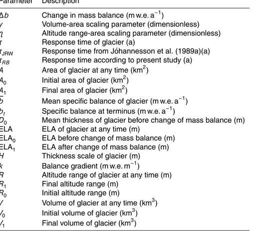
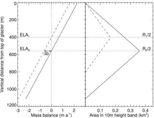
For a glacier in equilibrium with climate the mean specific mass balance, i.e. the area-averaged balance for the whole glacier (Anonymous, 1969) is zero. Its equilibrium line 20

altitude (ELA) is ELA₀and its dimensions are constant with time (see Table 1 for model notation). The glacier has areaA0and volumeV0. The mass balance is then suddenly

perturbed by∆bapplied over the whole area of the glacier and the ELA instantly rises to ELA₁, and the dimensions of the glacier slowly change to bring the glacier back into a new equilibrium state with areaA1and volumeV1.

25

(6)

TCD

3, 243–275, 2009

Title Page

Tables Figures

◭ ◮

Back Close

Full Screen / Esc

Interactive Discussion we assume is linear over the whole glacier. The new ELA of the glacier, ELA1, depends

upon the magnitude of the mass balance perturbation and the balance gradientk, such that:

ELA₁₌ELA₀₊∆b

k (2)

Figure 1 is drawn for a typical alpine glacier where a temperature rise of+1 K through-5

out the whole year causes a mass balance change of−0.66 m watera−1and raises the ELA by 160 m (values from the model calculations for Braithwaite and Raper, 2007). The change in mass balance for a 1 K temperature rise is termed the temperature sen-sitivity of mass balance (Oerlemans and Fortuin, 1992; Braithwaite and Zhang, 1999; de Woul and Hock, 2005). Equation (2) could be applied to a mass balance change due 10

to precipitation change and we would then use the precipitation sensitivity of mass bal-ance. For the present paper we abbreviate “temperature sensitivity of mass balance” to ‘mass balance sensitivity’ because we are only dealing with temperature changes.

Our conceptual model is simple but not unrealistic:

1. Balance gradients are not generally constant with altitude on real glaciers, reflect-15

ing effects of precipitation variations as well as wind drifting and avalanches. Bal-ance gradients are also greater in the ablation area and smaller in the accumula-tion area (Furbish and Andrews, 1984; Braithwaite and Raper, 2007). We assume a constant balance gradient here to derive an analytical solution for glacier volume change but for numerical modelling we can use the degree-day model to calculate 20

non-linear balance-altitude relations, e.g. as in Braithwaite and Raper (2007).

2. Figure 1 shows triangular area-altitude distributions that are symmetrical about the ELA (Raper and Braithwaite, 2006) and we also assume that the glacier re-tains a symmetrical altitude distribution as it shrinks. We return to these points later in the paper with data from real glaciers to show these are reasonable first 25

(7)

TCD

3, 243–275, 2009

Title Page

Tables Figures

◭ ◮

Back Close

Full Screen / Esc

Interactive Discussion 3. The apex of the triangle in Fig. 1 is the median altitude of the glacier, dividing the

glacier area into equal halves, and this coincides with the ELA when the glacier is in equilibrium (Meier and Post, 1962; Braithwaite and M ¨uller, 1980). For a symmetric altitude distribution, the median altitude is also equal to the area-weighted mean altitude of the glacier (Kurowski, 1893).

5

4. For a linear balance-gradient, the specific mass balance at the median altitude (also the mean altitude) is equal to the mean specific mass balance (Kurowski, 1893; Braithwaite and M ¨uller, 1980).

5. The assumption of linear balance-gradient is not as restrictive as it may first ap-pear because glacier areas are generally largest near the median altitude, where 10

there is maximum ice flux, and smallest at the top and bottom of the glacier where the linear assumption is most likely to be violated. The k parameter in Eq. (2) should therefore be regarded as representing the balance gradient near the ELA, i.e. the activity index of Meier (1962) or the energy of glacierization of Shum-sky (1947).

15

We measure all heights downwards from the top of the glacier which is assumed fixed when climate changes. This is a reasonable assumption for valley and moun-tain glaciers whose tops are constrained by hard rock topography but does not apply to ice caps since the maximum height of an ice cap changes with the ice cap thick-ness. The approach used in this paper does not therefore apply to ice caps. As the 20

maximum altitude of the glacier is fixed, shrinkage of the glacier involves a rise in the minimum elevation, or a reduction in the altitude rangeR between maximum and mini-mum altitudes of the glacier. As the glacier’s area and volume shrink towards the new equilibrium state, the half-range (R/2) moves from R0/2 at the old ELA toR1/2 at the

new ELA. The mass balancebof the whole glacier at any time is then equal to: 25

b=k(R1−R)

(8)

TCD

3, 243–275, 2009

Title Page

Tables Figures

◭ ◮

Back Close

Full Screen / Esc

Interactive Discussion Equation (3) follows from Eq. (2) when the initial mass balance perturbation,∆b, and

initial altitude rangeR0, are replaced by the time-evolving variablesbandR. Measuring

heights downwards,R is bigger thanR1andbis therefore negative and tends to zero

asR approachesR1.

The mass balance at the glacier terminus (altitudeR measured from the top of the 5

glacier) at any time after the mass balance perturbation is given by

bt=k

_R

0

2

−R

+ ∆b (4)

The mass balance at the terminus is therefore a function of both climate (balance gradient, k) and glacier geometry (altitude range, R) and changes until it achieves a new steady-state value forR=R1. The value of R1 can be calculated from Eq. (2) by

10

noting that ELA1=R1/2 and ELA0=R0/2 which gives:

R₁=R₀+2

∆b k

(5)

The total change in altitude of the terminus according to Eq. (5) is twice the change in ELA in Eq. (2). We return to the issue of the mass balance at the terminus at the end of this section and in a later section but start our analysis with the mean specific balance. 15

The product of the glacier areaAand mean specific balance, given by Eq. (3), gives the rate of change of glacier volume:

d V d t =Ak

(R1−R)

2 (6)

We treat ice dynamics implicitly by using geometric scaling following Chen and Ohmura (1990), Bahr et al. (1997), Raper et al. (1996, 2000), Van de Wal and 20

Wild (2001), Raper and Braithwaite (2006) and Radic et al. (2007, 2008). We follow others in assuming that volume scales onto area as

(9)

TCD

3, 243–275, 2009

Title Page

Tables Figures

◭ ◮

Back Close

Full Screen / Esc

Interactive Discussion and we use a scaling relation between altitude range and area as implemented by

Raper and Braithwaite (2006) so that

R∝Aη. (8)

Bahr et al. (1997) estimate the scaling indexγin Eq. (7) from depth-sounding observa-tions on 144 glaciers and obtain an average of 1.36, which is in remarkable agreement 5

with Chen and Ohmura (1990) who studied fewer glaciers. Bahr et al. (1997) also quote Russian authors for indices in the range 1.3 to 1.4. Paterson (1981, 1994) gives indices of 1.25 and 1.5, respectively, for theoretical profiles of ice caps and valley glaciers. The volume-area scaling of Bahr et al. (1997) has been criticised as it “correlates a statisti-cal variable (area) with itself (area in volume)” (Haeberli et al., 2007; L ¨uthi et al., 2008) 10

but we think it is a good example of an empirical relation with a sound physical back-ground. The γ value is greater than unity because average glacier depth increases with increasing glacier area.

From Eqs. (7 and 8) expressions for Aand R can be derived in terms of V andV0,

giving: 15

A=A0

_V

V₀

1_γ

(9)

R=R0

_V

V0

η_γ

(10)

Substitution of Eqs. (9 and 10) into Eq. (6) gives a new form of the volume change equation:

d V d t =A0

V V0

1_γ

k

_R

0

2

"_V

1

V0

η_γ

−

V V0

η_γ#

(11) 20

If we now define a new volume variableY by:

(10)

TCD

3, 243–275, 2009

Title Page Abstract Introduction Conclusions References Tables Figures ◭ ◮ ◭ ◮ Back Close

Full Screen / Esc

Interactive Discussion Then Eq. (11) may be written in more conventional linear-response form involving a

time scale,τ, as:

d Y d t =

(Y1−Y)

τ (13)

WhereY1andY areV η/γ 1 andV

η/γ

, respectively. Y refers to the current glacier volume while Y1 refers to the new equilibrium volume towards which the current volume is

5

tending. The glacier volume response time,τ, is defined as:

τ= _γ η D0 2 R₀ 1 k V V₀

(γ−1_γ−η)

(14)

where the mean glacier depth D0 equals V0/A0. The last term determines how the

response time changes non-linearly with changing volume. However, for a glacier in or near its reference state, i.e.V≈V0for small volume changes, the equation is simplified

10

because the fifth term becomes unity:

τ= _γ η D0 2 R0 1 k (15)

This is the form of the equation that we use later in the paper. However, it is useful to briefly compare our formulation with that of J ´ohannesson et al. (1989a). A more in-depth comparison is made in a later section.

15

In Eq. (15) the first term (γ/η) involves the scaling factors, the second term (D0)

represents glacier geometry before perturbation of mass balance, and according to Eq. (4) the inverse of the third and fourth term k.(R0/2) represents −bt where bt is

the balance at the terminus before perturbation of mass balance. Our response time Eq. (15) can therefore be expressed by:

20

τ=

_γ

η

D0

−bt

(11)

TCD

3, 243–275, 2009

Title Page

Tables Figures

◭ ◮

Back Close

Full Screen / Esc

Interactive Discussion Comparing Eq. (16) with Eq. (1) from J ´ohannesson et al. (1989a), shows that both

equations involve a ratio of glacier depth to balance at the terminus but our equation for response time Eq. (16) involves an extra numerical factor of (γ/η).

2.1 The effects of climate change

The effects of climate change on glacier volume are expressed by the mass balance 5

sensitivity and the response time. The former defines the immediate change in mass balance caused by a particular change in temperature and the latter measures the speed at which the glacier volume adjusts to the climate change. The response time depends upon the mass balance gradient according to Eq. (15) as well as upon glacier dimensions.

10

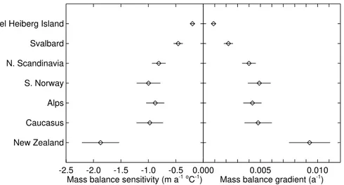
We use mass balance sensitivities and gradients calculated with a degree-day model for seven regions (Braithwaite and Raper, 2007). The degree-day model is applied to the estimated ELA for half-degree latitude-longitude grid squares contain-ing glaciers within each region. The estimated ELA for each grid square is the av-erage of median altitude for all glaciers within the grid square. The regions (Ta-15

ble 2) were chosen for their good data coverage in the World Glacier Inventory (http://nsidc.org/data/glacier inventory). They include the five main glacial regions of Europe together with Axel Heiberg Island, Canada, and New Zealand, which were added to represent the extremes of cold/dry and warm/wet conditions.

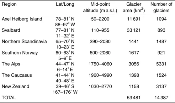
Average and standard deviation of mass balance sensitivity and gradient are shown 20

in Fig. 2 for the seven regions. The mass balance sensitivity and balance gradient both vary by about an order of magnitude. The mass balance model gives a very strong negative linear relationship between the mass balance sensitivity and the mass balance gradient (r=−1.00) with low (negative) sensitivity and low gradient in dry-cold conditions and high (negative) sensitivity and high gradient in wet-warm conditions. 25

(12)

TCD

3, 243–275, 2009

Title Page

Tables Figures

◭ ◮

Back Close

Full Screen / Esc

Interactive Discussion between mass balance sensitivity and mass balance gradient are to a large extent

governed by the temperature lapse rate, see Kuhn (1989).

The link between the mass balance sensitivity and the glacier volume response time (through the mass balance gradient) has implications for long-term changes in glacier volume and global sea-level. It means that warm/wet glaciers with large mass balance 5

sensitivity tend to have a small response time whereas cold/dry glaciers with small mass balance sensitivity tend to have a longer response time. This behaviour was noted by Raper et al. (2000) in sensitivity experiments. Thus temperature-sensitive glaciers show the most rapid response to climate change at present but may not be the most important contributors to sea level change in the long term.

10

3 The effects of topography

In this section, we analyse the World Glacier Inventory data to estimate the area vs al-titude scaling index values appropriate for the seven regions with their particular topo-graphic relief. The World Glacier Inventory data mostly originates from measurements taken in the third quarter of the 20th Century (∼1950–1975). This was a time of relative 15

glacier stability and the worldwide mass balance was generally smaller (closer to zero) than more recently (Kaser et al., 2006). First, however, we examine the validity of our assumption of triangular and symmetric area vs altitude distribution.

The World Glacier Inventory (http://nsidc.org/data/glacier inventory) is coded ac-cording to the instructions of M ¨uller et al. (1977). There are data for a total of 14 387 20

glaciers covering a total area of 53 481 km2for the seven regions (Table 2). This rep-resents less than 10% of all the mountain glaciers and ice caps on the globe, most of which are still not included in the World Glacier Inventory. For the present study, the required variables are area, maximum, minimum, and median elevation and primary classification for each glacier.

25

(13)

TCD

3, 243–275, 2009

Title Page

Tables Figures

◭ ◮

Back Close

Full Screen / Esc

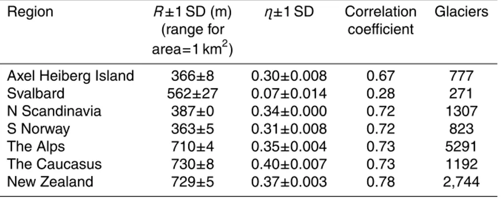
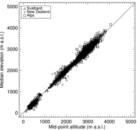
Interactive Discussion and M ¨uller (1980). We can then compare the median altitude (properly defined) with

the mid-point altitude representing the average of maximum and minimum glacier al-titudes (note that many authors incorrectly use the term median for the latter). The difference between median and mid-point altitude is a measure of the asymmetry of the area-altitude distribution. There are missing data for one or other altitude for many 5

glaciers. For example, data are not available at all for median altitude for regions 1, 3 and 4 (Axel Heiberg Island, Northern Scandinavia and Southern Norway), and for region 6 (Caucasus) the listed median altitudes are identical to the mid-point altitudes. Glacier inventories for these areas were finished before the instructions of M ¨uller et al. (1977) were available, thus accounting for the omission of median elevation (re-10

gions 1, 3 and 4) or its wrong definition (region 6).

The comparison between median and mid-point altitudes could be made for 6976 glaciers in three of the seven regions. However, our conceptual model (Fig. 1) does not apply to “ice caps” and to “outlet glaciers” and we exclude them from the data set, i.e. glaciers with primary classification equal to 3 and 4 according to M ¨uller et 15

al. (1977). Median altitude can then be compared with mid-point altitude for 6831 glaciers. On average there is a remarkably good agreement, with very little difference (mean and standard deviation) between the two altitudes compared with the altitude range of glaciers (Table 3). There is also a high correlation and nearly 1:1 relation between the two altitudes (Fig. 3). The assumption of a symmetrical altitude-area 20

distribution in our conceptual model is therefore very sound within a few decametres, e.g. the root-mean-square error of the regression line in Fig. 4 is only ±61 m. We believe that glacier area-altitude distributions may actually be somewhat asymmetric during periods of advance or retreat but the overall effect (Table 3) is small: presumably the sample of 6831 glaciers contains a mixture of retreating, stationary and advancing 25

glaciers.

(14)

TCD

3, 243–275, 2009

Title Page

Tables Figures

◭ ◮

Back Close

Full Screen / Esc

Interactive Discussion can differ in their response times due to different geometry. This can be thought of as

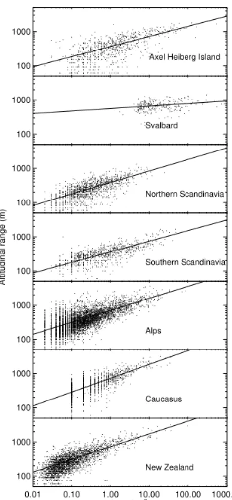
noise superimposed on a common signal of glacier response in a region determined by the regional climate and topography. In the empirical derivation of regional scaling indices that follows, we assume that a typical glacier growing or shrinking in a region will in general still have its geometrical dimensions governed by that region’s topographical 5

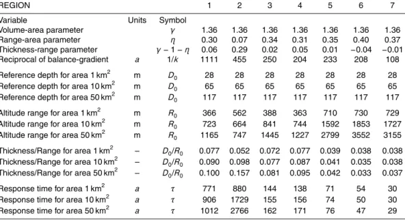
relief. According to the scaling relation (Eq. 8), altitude range is linked to area and we estimate the scaling parameter ηby regression analysis of data from the glacier inventory. There are two ways that this could be done: nonlinear regression with the original data for range and area or linear regression with logarithms of range and area. Results are fairly similar but we think the first approach gives better fit to the larger 10

glaciers. Statistical results for the nonlinear regression equation R∝Aη are given in Table 4 for each of the seven regions. The regression lines from the nonlinear analysis are re-plotted as straight lines in log-log space in Fig. 4 to illustrate the overall fit of the data.

The estimated values of η in Table 4 are rather similar (0.3 to 0.4) for six of the 15

regions but relatively low (0.07) for Svalbard. The latter is clearly anomalous and must be partly due to the omission of smaller glaciers (<1 km2) from the glacier inventory compared with the other regions in Fig. 4. As well as supplying us with estimates of ηfor our response time Eq. (15), the regression analysis allows us to identify typical altitude ranges for a selection of glacier areas to explore response times for generic 20

glaciers (see below).

4 The volume response time for seven regions

Using the formula for volume response time τ in Eq. (15) we make calculations for some generic glaciers to illustrate the effects of differing geometry and climate regime (Table 5). Results are calculated for glacier areas of 1, 10, 50 km2, respectively, with 25

(15)

TCD

3, 243–275, 2009

Title Page

Tables Figures

◭ ◮

Back Close

Full Screen / Esc

Interactive Discussion the region in question.

Some work on response time has suggested it should increase with glacier size, e.g. Table 13.1 in Paterson (1994), but Bahr et al. (1998) found that under certain conditions the response time will decrease as size increases. In seeming confirmation of this, Oerlemans et al. (1998) found “No straightforward relationship between glacier 5

size and fractional change of ice volume”. In our Table 5 response time does increase with area for regions 1 and 2 (Axel Heiberg Island and Svalbard), hardly increases in regions 3, 4 and 5 (Northern Scandinavia, Southern Norway and the Alps), and decreases in regions 6 and 7 (Caucasus and New Zealand). The reasons for this can be understood by looking at the detailed breakdown in Table 5.

10

The reciprocal of balance gradient in line 4 of Table 5 has the units of time (a) and expresses the basic effect of climate on response time with a range of 102to 103a, from the warm-wet (maritime) climate of New Zealand to the cold-dry (continental) climate of Axel Heiberg Island. Regions 1 and 2 both represent arctic islands but region 1 is obviously more continental than region 2. Balance gradients in regions 3, 4, 5 and 6 15

are quite similar while there is a further jump to the very maritime climate of region 7. This order of magnitude climate influence on the glacier volume response time is then modified by geometric factors.

With reference to Table 5, the geometric factorR0differs by a factor of 3 between

re-gions 1–4 and rere-gions 5–7 and has a corresponding influence on the volume response 20

times. The geometric factor that determines how the volume response time depends on glacier size is the depth-range ratio,D0/R0 (the middle terms of Eq. 15), which scales

asAγ₀−1−η. In Table 5, the indexγ−1−ηis either small positive or small negative, aside from anomalous results for region 2 (Svalbard). Examination of Table 5 shows that for the regions with negative indexγ−1−η,D0/R0decreases with increasing glacier area,

25

leading to shorter response times for larger glaciers in regions 6 and 7.

(16)

TCD

3, 243–275, 2009

Title Page

Tables Figures

◭ ◮

Back Close

Full Screen / Esc

Interactive Discussion values ofηindicate rapidly increasing altitudinal range with increasing glacier area and

may be associated with steeper terrain as suggested by Raper and Braithwaite (2005, 2006). We hope to explore this issue in a future study using data from other regions with even greater altitude ranges.

We are not able to di_fferentiate between di_fferent regions in our volume-area scaling 5

and we simply use the scaling factorγ=1.36 from Bahr et al. (1997). This means we have to assume a single glacier depth for a particular area in Table 5 but we speculate that a regionally-specific glacier depth would further increase the range of response times shown in Table 5. The reasoning is that glaciers in regions with high topographic relief, with large altitude ranges, are likely to be faster flowing and thinner (smallerD0)

10

than those in relatively flat terrain, thus further reducing already short response times.

5 An alternative approach

We start by returning to the definition of volume response timeτ in J ´ohannesson et al. (1989a):

τ=∂V

∂B (17)

15

Where∂V is the di_fference in the steady state volume of the glacier before and after the mass balance perturbation, and∂Bis the integral of the mass balance perturbation over the initial area of the glacier. J ´ohannesson et al. (1989a) then give expressions for these terms for some simplified glacier geometries. Their crucial assumption is that the initial mass balance perturbation of the whole glacier is balanced in the new steady 20

state by an area change at the glacier terminus over which the mean specific mass balance is the initial mass balance at the terminus bt. We, however, can apply our

conceptual model to Eq. (17) as follows:

(17)

TCD

3, 243–275, 2009

Title Page Abstract Introduction Conclusions References Tables Figures ◭ ◮ ◭ ◮ Back Close

Full Screen / Esc

Interactive Discussion ∂B=A0k

(R1−R0)

2 (19)

Where ∂B refers to the volumetric balance obtained by multiplying specific balances from Eq. (3) by glacier area.

Substituting the volume-area scaling Eq. (9) into Eq. (18) gives:

∂V =V0

_A 1 A0 γ −1 (20) 5

For relatively small area changes, we can use a truncated McLaurin series to replace (A1/A0)

γ

with 1-γ [1-(A1/A0)]. Substituting this linear approximation back into Eq. (20),

with re-arrangement and expressingV0/A0as the mean depth of the glacierD0gives:

∂V =D0γ

A1−A0

(21)

In a similar way: 10

∂B=k

_R

0

2

η

A1−A0

(22)

Dividing Eq. (20 by 21) then gives us

τ=

D0γ

h kR0

2

ηi

(23)

This is identical to our original derivation in Eq. (15).

From an inspection of Eqs. (10 and 11) in J ´ohannesson et al. (1989a), and translating 15

into our notation, his thickness scaleH is given by:

H = _{d V} d A A0 V0

(18)

TCD

3, 243–275, 2009

Title Page

Tables Figures

◭ ◮

Back Close

Full Screen / Esc

Interactive Discussion WhereD0 is the mean depth of the glacier. J ´ohannesson et al. (1989a) evaluate the

expression (dV/dA) (A0/V0) in terms of analytical solutions for simplified glacier

geom-etry. We now evaluate this expression using the volume-area scaling method that was not available in its present form in 1989. ExpressingV asV0(A/A0)

γ

and differentiating with respect toA, we find (dV/dA) (A0/V0)=γ. Therefore:

5

H =γD0 (25)

Substitution of Eq. (25) back into Eq. (1) gives the response time of J ´ohannesson et al. (1989a) as:

τJRW=

γD0

−bt

(26)

WhereτJRWdenotes the response time according to J ´ohannesson et al. (1989a).

10

Comparing Eq. (26) with (16) shows that:

τ_RB = τJRW_η (27)

Where τ_RB is the response time according to the present authors Raper and Braith-waite.

6 Discussion 15

Using a mid estimate of ηof 0.36, our response time τ_RB is about 2.8 (1/0.36=2.78) times longer thanτJRW, the response time of J ´ohannesson et al. (1989a). Anηvalue

of unity (R∝A) is implicit in the glacier of unit or uniform width with all area changes at the terminus assumed by J ´ohannesson et al. (1989a). Radic et al. (2007) also used a glacier of uniform width (and slope) in a comparison of a flow line model with a scaling 20

model.

(19)

TCD

3, 243–275, 2009

Title Page

Tables Figures

◭ ◮

Back Close

Full Screen / Esc

Interactive Discussion distribution for different values of η when the area shrinks fromA0 toA1. Forη>0.5,

a large reduction in range toR1 would result in the dashed line aboveR1/2, in Fig. 1,

being above the solid line joining the top of the glacier toR0/2. This is equivalent to a

raising of the glacier surface due to thickening in the accumulation area as the total area is reduced, which is clearly unrealistic. Forη=0.5, the solid and dashed lines above 5

R1/2 in Fig. 1 would coincide, implying no change in area or surface altitude above the

new ELA for a change in area fromA0to the smaller A1. The geometry changes that

occur forη<0.5 as shown in Fig. 1 are consistent with a lowering of the glacier surface due to thinning in both accumulation and ablation areas, when going from A0 to the

smallerA1. Thus the formulation of the model in the vertical area-altitude dimension

10

allows the mass balance-elevation feedback associated with both the area reduction and lowering of the glacier surface to be accounted for. Our empirically derived values ofηof 0.3–0.4 are consistent with the geometric expectations that η<0.5. In accord with our results, Oerlemans (2001, Table 8.3) found that, when applied to four real glaciers, his flow line model gave glacier volume response times that are longer than 15

implied by the J ´ohannesson et al. (1989a) formula. J ´ohannesson et al. (1989a, b) do realise that their crucial assumption (see above) means that balance-elevation feed-back is not accounted for and that their response time estimates may therefore be too short. Harrison et al. (2001) attempt to correct this by including a term that explicitly ad-dresses the balance-elevation feedback, but they still assume that all the area change 20

is close to the terminus. Their treatment cannot account for area-altitude changes due to thickening/thinning of the glacier far removed from the region of the terminus, i.e. in the accumulation area.

Our modelling of both mass balance and glacier area in the vertical dimension means that the mass balance elevation feedback resulting from both changes in total area and 25

(20)

TCD

3, 243–275, 2009

Title Page

Tables Figures

◭ ◮

Back Close

Full Screen / Esc

Interactive Discussion i.e. the glacier area may change, but the thickness along the glacier profile does not”.

We find this statement puzzling since logically changes in the area-elevation distribu-tion should reflect changes in glacier thickness.

Due to lack of data we are not able to estimate regionally specific values for γ, though we might expect lower/higher values of γ to be associated with lower/higher 5

topographic relief. This issue should be resolved by extending the dataset by depth-sounding or other means (Farinotti et al., 2008) of estimating glacier volume for many more glaciers, especially in regions with high topographic relief. We note that changes in sub-glacial hydrology or in thermal conditions at the glacier bed may also have an effect onγ.

10

7 Conclusions

We propose a new derivation of the volume response time where the climate and geometric parameters are separated. The volume response time depends directly upon the mean glacier thickness, and indirectly on glacier altitude range and vertical mass-balance gradient. Our formula can be reduced to the well-known ratio of glacier 15

thickness to mass balance at the glacier terminus (J ´ohannesson et al., 1989a) but involves an extra numerical factor. This factor increases our volume response time by a factor of about 2.8 compared with that of J ´ohannesson et al. (1989a) and reflects the mass balance elevation feedback.

Because volume response time depends upon vertical mass balance gradient, 20

warm/wet glaciers tend to have shorter response times and cold/dry glaciers tend to have longer response times.

Our model is derived for glaciers whose area distribution is assumed to be symmet-rical around the equilibrium line altitude (ELA). It is long known that in steady-state the ELA is approximately equal to median glacier altitude and we now confirm that the 25

mid-point altitude is approximately equal to median altitude.

(21)

re-TCD

3, 243–275, 2009

Title Page

Tables Figures

◭ ◮

Back Close

Full Screen / Esc

Interactive Discussion gions such that volume response time can increase with area (Axel Heiberg Island and

Svalbard), hardly change (Northern Scandinavia, Southern Norway and the Alps), or even get smaller (Caucasus and New Zealand).

Acknowledgements. The authors are indebted to Tim Osborn, Climatic Research Unit,

Univer-sity of East Anglia, for many useful discussions. Roger Braithwaite’s main work on this paper 5

was made during a period of research leave from the University of Manchester and he thanks colleagues for covering his teaching and administration duties.

References

Anonymous: Mass-balance terms, J. Glaciol., 8(52), 3–8, 1969.

Bahr, D. B.: Width and length scaling of glaciers, J. Glaciol., 43(145), 557–562, 1997. 10

Bahr, D. B., Meier, M. F., and Peckham, S. D.: The physical basis of glacier volume-area scaling, J. Geophys. Res., 102, 20355–20362, 1997.

Bahr, D. B., Pfeffer, W. T., Sassolas, C., and Meier, M.: Response time of glaciers as a function of size and mass balance: 1. Theory, J. Geophys. Res., 103, 9777–9782, 1998.

Braithwaite, R. J. and M ¨uller, F.: On the parameterization of glacier equilibrium line altitude. 15

World Glacier Inventory – Inventaire mondial des Glaciers (Proceeding of the Riederalp Workshop, September 1978: Actes de l’Ateliere de Riederalp, september 1978), IAHS-AISH, 127, 273–271, 1980.

Braithwaite, R. J. and Zhang, Y.: Modelling changes in glacier mass balance that may occur as a result of climate changes, Geogr. Ann. A, 81(4), 489–496, 1999.

20

Braithwaite, R. J. and Raper, S. C. B.: Glaciological conditions in seven contrasting regions estimated with the degree-day model, Ann. Glaciol., 46, 297–302, 2007.

Callendar, G. S.: Note on the relation between the height of the firn line and the dimensions 0f a glacier, J. Glaciol., 1(8), 459–461, 1950.

Callendar, G. S.: The effect of the altitude of the firn area on a glacier’s response to temperature 25

variations, J. Glaciol., 1(10), 573–576, 1951.

Chen, J. and Ohmura, A.: Estimation of alpine glacier water resources and their change since the 1870s, IAHS Publ., 193, 127–135, 1990.

De Woul, M. and Hock, R.: Static mass-balance sensitivity of arctic glaciers and ice caps using a degree-day approach, Ann. Glaciol., 42, 217–224, 2005.

(22)

TCD

3, 243–275, 2009

Title Page

Tables Figures

◭ ◮

Back Close

Full Screen / Esc

Interactive Discussion Farinotti, D., Huss, M., Bauder, A., Funk, M., and Truffer, M.: A method to estimate ice volume

and ice thickness distribution of alpine glaciers, J. Glaciol., in press, 2008.

Furbish, D. J. and Andrews, J. T.: The use of hypsometry to indicate long-term stability and response of valley glaciers to changes in mass transfer, J. Glaciol., 30(105), 199–211, 1984. Haeberli, W., Hoelzle, M., Paul, J., and Zemp, M.: Integrated monitoring of mountain glaciers 5

as key indicators of global climate change: the European Alps, Ann. Glaciol., 46, 150–160, 2007.

Harrison, W. D., Elsberg, D. H., Echelmeyer, K. A., and Krimmel, R. M.: On the characterization of glacier response by a single time-scale, J. Glaciol., 47(159), 659–664, 2001.

Huybrechts, P., Payne, T., and the EISMINT Intercomparison Group: The EISMINT benchmarks 10

for testing ice-sheet models, Ann. Glaciol., 23, 1–12, 1996.

IPCC, Climate Change: The Physical Sciences Basis, Contribution of Working Group I to the Fourth Assessment Report of the Intergovernmental Panel on Climate Change, edited by: Solomon, S., Qin, D., Manning, M., Chen, Z., Marquis, M., Averyt, K. B., Tignor, M., and Miller, H. L., Cambridge University Press, Cambridge, UK and New York, NY, USA, 996 pp., 15

2007.

J ´ohannesson, T., Raymond, C. F., and Waddington, E. D.: A simple method for determining the response time of glaciers, J. Oerlemans ed. Glacier Fluctuations and Climate Change, Kluwer, 407–417, 1989a.

J ´ohannesson, T., Raymond, C. F., and Waddington, E. D.: Time-scale for adjustments of 20

glaciers to changes in mass balance ,J. Glaciol., 35(121), 355–369, 1989b.

Kaser, G., Cogley, J. G., Dyurgerov, M. B., Meier, M. F., and Ohmura, A.: Mass balance of glaciers and ice caps: Consensus estimates for 1961-2004, Geophys. Res. Lett., 33, L19501. doi:10.1029/2006GL027511, 2006.

Kuhn, M.: The response of the equilibrium line altitude to climate fluctuations: theory and 25

observations, J. Oerlemans ed. Glacier Fluctuations and Climate Change, Kluwer, 407–417, 1989.

Kurowski, L.: Die H ¨ohe der Schneegrenze mit besonderer Ber ¨ucksichtigung der Finsteraarhorne-Gruppe, Penck’s Geogr., Abhandlungen, 5(1), 119–160, 1893.

L ¨uthi, M., Funk, M., and Bauder, A.: Comment on “Integrated monitoring of mountain glaciers 30

as key indicators of global climate change: the European Alps” by Haeberli et al., J. Glaciol., 54(184), 199–200, 2008.

(23)

TCD

3, 243–275, 2009

Title Page

Tables Figures

◭ ◮

Back Close

Full Screen / Esc

Interactive Discussion 1962.

Meier, M. F.: Contribution of small glaciers to global sea level, Science, 227, 1418–1421, 1984. Meier, M. F. and Post, A. S.: Recent variations in mass net budgets of glaciers in western North

America, Variations du regime des glaciers existants – Variations of the regime of existing glaciers, Proceeding of the Obergurgl Symposium, September 1962, IAHS-AISH, 58, 63–77, 5

1962.

M üller, F., Caflisch, T., and M üller, G.: Instructions for the compilation and assemblage of data for a world glacier inventory, Z ürich, ETH Z ürich, Temporary Technical Secretariat for the World Glacier Inventory, 293 pp., 1977.

Nye, J. F.: The flow of glaciers, Nature, 161, 4099, 819–821, 1948. 10

Nye, J. F.: On the theory of the advance and retreat of glaciers, Geophys. J. Roy. Astr. S., 7(4), 431–456, 1963.

Pfeffer, W. T., Sassolas, C., Baht, D. B, and Meier, M.: Response time of glaciers as a function of size and mass balance: 2. Numerical experiments, J. Geophys. Res., 103, 9777–9782, 1998.

15

Oerlemans, J. and Fortuin, J. P. F.: Sensitivity of glaciers and small ice caps to Greenhouse warming, Science, 258, 115–117, 1992.

Oerlemans, J.: Modelling of glacier mass balance, in: Ice in the climate system, edited by: Peltier, W. R., Berlin and Heidelberg, Springer-Verlag, 101–116, 1993.

Oerlemans, J., Anderson, B., Hubbard, A., Huybrechts, P., J ´ohannesson, T., Knap, W. H., 20

Schmeits, M., Stroeven, A. P., van de Wal, R. S. W., Wallinga, J., and Zuo, Z.: Modelling the response of glaciers to climate warming, Clim. Dynam., 14, 277–274, 1998.

Oerlemans, J.: Glaciers and climate change, Lisse, etc., A. A. Balkema, 148 pp., 2001. Oerlemans, J.: Estimating response times of Vadret da Morteratsch, Vadret da Palu,

Briksdals-breen and NigardsBriksdals-breen from their length records, J. Glaciol., 53(182), 357–362, 2007. 25

Paterson, W. S. B.: Laurentide ice sheet: estimated volumes during the late Wisconsin, Review of Geophysics and Space Physics, 10, 885–917, 1972.

Paterson, W. S. B.: The physics of glaciers. (2nd edition), Pergamon, Oxford, 380 pp., 1981. Paterson, W. S. B.: The physics of glaciers. (3rd edition), Pergamon, Oxford, UK, 480 pp.,

1994. 30

Radic, V., Hock, R., and Oerlemans, J.: Volume-area scaling vs. flowline modelling in glacier volume projections, Ann. Glaciol., 46, 234–240, 2007.

(24)

TCD

3, 243–275, 2009

Title Page

Tables Figures

◭ ◮

Back Close

Full Screen / Esc

Interactive Discussion evolutions of valley glaciers, J. Glaciol., 5(187), 1–12, 2008.

Raper, S. C. B., Briffa, K. R., and Wigley, T. M. L.: Glacier change in northern Sweden from AD500: a simple geometric model of Storglaci ¨aren, J. Glaciol., 42(141), 341–351, 1996. Raper, S. C. B., Brown, O., and Braithwaite, R. J.: A geometric glacier model for sea level

change calculations, J. Glaciol., 46(154), 357–368, 2000. 5

Raper, S. C. B. and Braithwaite, R. J.: The potential for sea level rise: new estimates from glacier and ice cap area and volume distributions, Geophys. Res. Lett., 32(7), L05502, doi:10.1029/2004GL021981, 2005.

Raper, S. C. B. and Braithwaite, R. J.: Low sea level rise projections from mountain glaciers and icecaps under global warming, Nature, 439, 7074, 311–313, 2006.

10

Shumsky, P. A.: The energy of glacierization and the life of glaciers, English translation by: Kotlyakov, V. M. (ed.), 1997, 34 Selected papers on main ideas of the Soviet Glaciology, 1940a–1980s, Moscow, Russian Academy of Sciences, 1947 (in Russian).

Van de Wal, R. S. W. and Wild, M.: Modelling the response of glaciers to climate change by applying the volume-area scaling in combination with a high resolution GCM, Clim. Dynam., 15

18, 359–366, 2001.

Warrick, R. A. and Oerlemans, J.: Sea level rise, in: Climate change – The IPCC Scientific Sssessment, edited by: Houghton, J. T., Jenkins, G. J. and Ephraums, J. J., Cambridge University Press, Cambridge, UK, 358–405, 1990.

World Glacier Inventory, World Glacier Monitoring Service and National Snow and Ice Data 20

(25)

TCD

3, 243–275, 2009

Title Page

Tables Figures

◭ ◮

Back Close

Full Screen / Esc

Interactive Discussion Table 1.Description of model parameters.

Parameter Description

∆b Change in mass balance (m w.e. a−1

)

γ Volume-area scaling parameter (dimensionless) η Altitude range-area scaling parameter (dimensionless) τ Response time of glacier (a)

τJRW Response time from J ´ohannesson et al. (1989a)(a)

τ_RB Response time according to present study (a) A Area of glacier at any time (km2)

A₀ Initial area of glacier (km2) A₁ Final area of glacier (km2)

b Mean specific balance of glacier (m w.e. a−1

) b_t Specific balance at terminus (m w.e. a−1)

D₀ Mean thickness of glacier before change of mass balance (m) ELA ELA of glacier at any time (m)

ELA₀ ELA before change of mass balance (m) ELA₁ ELA after change of mass balance (m) H Thickness scale of glacier (m)

k Balance gradient (m w.e. m−1)

R Altitude range of glacier at any time (m) R1 Final altitude range (m)

R0 Initial altitude range (m)

(26)

TCD

3, 243–275, 2009

Title Page

Tables Figures

◭ ◮

Back Close

Full Screen / Esc

Interactive Discussion Table 2. Summary data for the seven glacier regions. Based on data from World Glacier

Inventory.

Region Lat/Long Mid-point Glacier Number of

altitude (m a.s.l.) area (km2) glaciers Axel Heiberg Island 78–81◦_N _50–2200 _{11 691} ₁₀₉₄

88–97◦_W

Svalbard 77–81◦_N _110–955 _{33 121} ₈₉₃

11–32◦E

Northern Scandinavia 65–70◦N 290–2080 1441 1487 13–23◦E

Southern Norway 60–63◦_N _600–2060 ₁₆₁₇ ₉₂₁

5–9◦_E

The Alps 44–47◦_N _1750–4060 ₃₀₅₆ ₅₃₃₁

6–14◦_E

The Caucasus 41–44◦_N _1960–4990 ₁₃₉₈ ₁₅₂₄

40–48◦_E

New Zealand 39–46◦_S _1030–2770 ₁₁₅₈ ₃₁₃₇

167–176◦_W

(27)

TCD

3, 243–275, 2009

Title Page

Tables Figures

◭ ◮

Back Close

Full Screen / Esc

Interactive Discussion Table 3. Asymmetry of altitude-area distributions as expressed by the median and mid-point

altitudes for 6831 glaciers (excluding ice caps).

Concept Mean and standard

deviation

Di_fference between median ₋3_±62 m and mid-point altitudes

(28)

TCD

3, 243–275, 2009

Title Page

Tables Figures

◭ ◮

Back Close

Full Screen / Esc

Interactive Discussion Table 4.Parameter results from non-linear regression between altitude rangeRand areaAfor

seven regions.

Region R±1 SD (m) η±1 SD Correlation Glaciers (range for coefficient

area=1 km2)

Axel Heiberg Island 366±8 0.30±0.008 0.67 777

Svalbard 562±27 0.07±0.014 0.28 271

N Scandinavia 387_±0 0.34_±0.000 0.72 1307

S Norway 363_±5 0.31_±0.008 0.72 823

The Alps 710_±4 0.35_±0.004 0.73 5291

(29)

TCD

3, 243–275, 2009

Title Page

Tables Figures

◭ ◮

Back Close

Full Screen / Esc

Interactive Discussion Table 5.Parameters and variables needed to calculate response times for three different values

of glacier area in seven different regions. Regions are (1) Axel Heiberg Island, (2) Svalbard, (3) Northern Scandinavia, (4) Southern Norway, (5) Alps, (6) Caucasus and (7) New Zealand.

REGION 1 2 3 4 5 6 7

Variable Units Symbol

Volume-area parameter γ 1.36 1.36 1.36 1.36 1.36 1.36 1.36 Range-area parameter η 0.30 0.07 0.34 0.31 0.35 0.40 0.37 Thickness-range parameter γ−1−η 0.06 0.29 0.02 0.05 0.01 −0.04 −0.01 Reciprocal of balance-gradient a 1/k 1111 455 250 204 233 208 108 Reference depth for area 1 km2 m D₀ 28 28 28 28 28 28 28 Reference depth for area 10 km2 m D0 65 65 65 65 65 65 65

Reference depth for area 50 km2 m D0 117 117 117 117 117 117 117

Altitude range for area 1 km2 m R0 366 562 388 363 710 730 729

Thickness/Range for area 1 km2 – D0/R0 0.077 0.052 0.072 0.077 0.039 0.038 0.038

(30)

TCD

3, 243–275, 2009

Title Page

Tables Figures

◭ ◮

Back Close

Full Screen / Esc

Interactive Discussion

-3 -2 -1 0 1 2

Mass balance (m a-1₎

1200 1000 800 600 400 200 0

Vertical distance from top of glacier (m)

∆b

ELA₀ ELA1

0.1 0.2 0.3 0.4

Area in 10m height band (km2₎

R₀/2 R1/2

(31)

TCD

3, 243–275, 2009

Title Page

Tables Figures

◭ ◮

Back Close

Full Screen / Esc

-2.5 -2.0 -1.5 -1.0 -0.5

Mass balance sensitivity (m a-1o

C-1

) New Zealand

Caucasus Alps S. Norway N. Scandinavia Svalbard Axel Heiberg Island

0.005 0.010

0.000

Mass balance gradient (a-1

)

(32)

TCD

3, 243–275, 2009

Title Page

Tables Figures

◭ ◮

Back Close

Full Screen / Esc

0 1000 2000 3000 4000 5000

Mid-point altitude (m a.s.l.) 0

1000 2000 3000 4000 5000

Median elevation (m a.s.l.)

Svalbard New Zealand Alps

(33)

TCD

3, 243–275, 2009

Title Page

Tables Figures

◭ ◮

Back Close

Full Screen / Esc

Interactive Discussion 100

1000

Axel Heiberg Island

100 1000

Svalbard

100 1000

Northern Scandinavia

100 1000

Altitudinal range (m)

Southern Scandinavia

100 1000

Alps

100 1000

Caucasus

0.01 0.10 1.00 10.00 100.00 1000.00 Area (km2

) 100

1000

New Zealand