Simulation of aerosol optical properties over Europe with a 3-D size-resolved aerosol model: comparisons with AERONET data

(1)

ACPD

8, 1321–1365, 2008

Simulation of aerosol optical properties

M. Tombette et al.

Title Page

Abstract Introduction

Conclusions References

Tables Figures

◭ ◮

Back Close

Full Screen / Esc

Printer-friendly Version

Interactive Discussion

EGU Atmos. Chem. Phys. Discuss., 8, 1321–1365, 2008

www.atmos-chem-phys-discuss.net/8/1321/2008/ © Author(s) 2008. This work is licensed

under a Creative Commons License.

Atmospheric Chemistry and Physics Discussions

Simulation of aerosol optical properties

over Europe with a 3-D size-resolved

aerosol model: comparisons with

AERONET data

M. Tombette1, P. Chazette2, and B. Sportisse1

1

CEREA, Research and Teaching Center in Atmospheric Environment, Joint Laboratory ´Ecole Nationale des Ponts et Chauss ´ees/EDF R&D, 77455 Champs sur Marne, France

2

LSCE, Laboratoire des Sciences du Climat et de l’Environnement, Joint Laboratory CEA-CNRS, 91191 Gif-Sur-Yvette, France

(2)

ACPD

8, 1321–1365, 2008

M. Tombette et al.

Title Page

Tables Figures

◭ ◮

Back Close

Full Screen / Esc

EGU

Abstract

This paper aims at presenting a model-to-data comparison of the Aerosol Optical Thick-ness (AOT) and of a few sparse data for Single Scattering Albedo (SSA) over Europe for one year. The optical parameters are computed from a size-resolved aerosol model embedded in the POLYPHEMUSsystem described inMallet et al.(2007). The method-5

ology is first described, showing that several hypothesis can be made for several mi-crophysical aerosol properties. The simulation is made over one year (2001); statistics and monthly time series for the simulation and AERONET data are used to evaluate the ability of the model to reproduce AOT and vertically averaged SSA fields and their variability. The relation with the uncertainties of measurements is discussed. Then a 10

sensitivity study with respect to the mixing state of the particle, the way to compute the Aerosol Complex Refractive Index (ACRI) of a mixture and the way to take into account water uptake is carried out. The results indicate that the computation of AOT is relatively stable, while the computation of the single scattering albedo is much more uncertain.

15

1 Introduction

Global warming by greenhouse gases is now well understood and can be assessed. The understanding of the impact of aerosols is a much more challenging issue. Aerosol physical processes and direct or indirect effects on the atmosphere are still an open research field and then roughly described in the models. The third and fourth reports 20

of the Intergovernmental Panel on Climate Change (IPCC,Houghton et al.,2001 and Forster et al., 2007) declare that for all these factors, there is no precise estimate of the radiative forcing by anthropogenic aerosols. Current estimates give a cooling of the earth’s surface, a warming of the atmosphere, and a negative budget at the top of atmosphere which is estimated to compensate part of the warming due to greenhouse 25

(3)

ACPD

8, 1321–1365, 2008

M. Tombette et al.

Title Page

Tables Figures

◭ ◮

Back Close

Full Screen / Esc

EGU vertical column, it has been pointed out that the aerosol global models should validate

and improve their vertical distribution. To access to this vertical information, compar-isons between observed and simulated Aerosol Optical Depth or Thickness (AOD/AOT) have been published for global models compared to satellite measurements or/and ground-based stations measurements (e.g.Chung et al.,2005;Chin et al.,2002; Pen-5

ner et al.,2002;Kinne et al.,2006;Yu et al.,2006;Ginoux et al.,2006). These models generally use fixed size distributions depending on the aerosol type (sea-salt, sulfate, etc.) in order to compute or tabulate aerosol extinction coefficients.

As the residence time of tropospheric aerosols ranges from 5 to 10 days (Seinfeld and Pandis, 1998), even 1 day in the atmospheric boundary layer, and as the pro-10

cesses governing aerosol physics are complex, it is also interesting to investigate the aerosol vertical distribution at a smaller scale. Regional effects are significant for ex-ample on the heating rate of the atmosphere (see INDOEX campaign Ramanathan et al., 2001). Also, as the key question about climate change deals with the effect due to anthropogenic activities, a special attention has to be paid to sulfate and black 15

carbon that have a cooling impact. For that interest, representation of urban areas is required, and the regional scale is more appropriate. Comparisons between satellite-derived and simulated AOT from Chemistry-Transport Models have also been made (e.g. Robles Gonz ´alez et al., 2003; Jeuken et al., 2001; Hodzic et al., 2004, 2006). Satellite measurements have the advantage that they provide horizontal information. 20

As the AERONET network accounts for 100 stations, with a large part in Europe, it is now possible to use it in the same way as the ground-based networks for PM10 have been used for validation. Moreover, AERONET AOT is used to validate AOT retrieved from satellite measurements: MODIS (Kaufman et al.,1997), POLDER (Deuz ´e et al., 2001), MeteoSat (Brindley and Ignatov,2006).

25

(4)

ACPD

8, 1321–1365, 2008

M. Tombette et al.

Title Page

Tables Figures

◭ ◮

Back Close

Full Screen / Esc

EGU temperature of the particle modifies water condensation (semi-direct effect, Lohmann

and Feichter,2005). This phenomenon also impacts cloud formation, so taking into account the feedback of aerosols on meteorology is also needed.

In this paper, we use a 3-D CTM (Polair3D, Boutahar et al., 2004) coupled with a size-resolved aerosol model (SIREAM, Debry et al., 2007) in the framework of 5

the POLYPHEMUS system (Mallet et al., 2007). The system has been evaluated for aerosol outputs (PM10, PM2.5 and chemical composition) and gase-phase species at the ground level for year 2001 over Europe (Sartelet et al., 2007) and over Greater Paris (Tombette and Sportisse, 2007). Two optical parameters (AOT and SSA) are computed from the simulation outputs and compared to AERONET data (this is a long-10

term comparison with several stations).

The objective of this paper is twofold. First, we want to perform a model-to-data comparison for a CTM on the basis of radiative data for a large ground-data basis. Second, a sensitivity study estimates the robustness of the simulated aerosol optical properties.

15

This paper is organized as follows. Different methods for the computation of AOT are described in Sect.2. They are based on parameterizations that depend on relative humidity (H ¨anel,1976;Gerber,1985) and that take advantage of the complexity of the model (size distribution and thermodynamics). The relative humidity has a great im-pact on chemistry and optical parameters of aerosols (Boucher and Anderson,1995; 20

Randriamiarisoa et al.,2006), which can be poorly described by parameterizations, as the H ¨anel one that does not take into account the hysteresis effect. Also, the different hypothesis made for the mixing state of the particles are considered. In Sect.3, we de-scribe the observational network AERONET used for AOT measurements. In Sect.4, the model configurations for the simulation over Europe are described. Then simulated 25

(5)

ACPD

8, 1321–1365, 2008

M. Tombette et al.

Title Page

Tables Figures

◭ ◮

Back Close

Full Screen / Esc

EGU

2 Computation of aerosol optical properties

As the model used to compute aerosols is a size-resolved model, outputs in one grid cell are the concentration of each aerosol species in each size section. Figure1shows the flow chart of the method used to compute AOT with model outputs and optical data. Each computing step is described hereafter.

5

2.1 General equations

AOT at a wavelengthλis defined as the integral of the extinction coefficientbextdue to particles through the atmosphere:

AOT(λ)=

Zz_TOA

zg

bext(λ, z)dz (1)

wherezTOAis the altitude at the Top Of Atmosphere andzgthe altitude at ground level. 10

The extinction coefficient is a function of the particle size, of the Aerosol Complex Refractive Index (referred as CRI or ACRI in the following paper)m and of the wave-lengthλ. For a polydisperse distribution of aerosols with the same ACRI m, the Mie theory (Mie,1908) gives the extinction coefficient by the following formula:

bext=

ZD_wetmax

0

πD2_wet

4 Qext(m, α)n(Dwet)dDwet (2)

15

whereDwet is the wet particle diameter, D max

wet the maximum wet diameter of the dis-tribution,αwet=

πD_wet

λ the size parameter, n(Dwet) the number size distribution function andQext(m, α) the extinction efficiency. The scattering coefficient is computed with the same formula from the scattering efficiencyQscatt(m, α).

The aerosol model is based on an assumption of internal mixing (aerosols in the 20

(6)

ACPD

8, 1321–1365, 2008

M. Tombette et al.

Title Page

Tables Figures

◭ ◮

Back Close

Full Screen / Esc

EGU and for each vertical level. The AOT computation will be based on the same hypothesis:

we consider that in each vertical layer, the aerosol population is divided intoNbingroups where the discretisation of the diameter spectrum is constant (geometric average of the bin bounds). Then, in one bin in one vertical layer, the aerosols have the same optical properties (Qextonly depends on the bini and the vertical layerk).

5

LetNbin be the number of bins labeled byi andNz be the number of vertical levels labeled byk. The discretization of Eqs. (1–2) leads to:

AOT(λ)₌ Nz

X

k=1

bext(λ, k)×(zk+1−zk) (3)

bext(λ, zk)= N_bin X

i=1

πD_wet2 _,i,k

4 Qext,i,kNi ,k (4)

where (z_k)_k₌1,Nz+1are the altitudes at the interface between the model layers andNi ,k

10

is the number of particle in the size bini in the vertical layerk.D_wet_,i,k andQ_ext_,i,kstand for the wet diameter and the extinction efficiency of bini in the layerk, respectively. 2.2 Computation of the dry ACRI

The computation of ACRI for a particle composed by several species should be made under an hypothesis on the mixing state of the particle. We propose here two mixing 15

states: the well-mixed case and the core hypothesis.

2.2.1 Well-mixed hypothesis

LetN_s be the number of chemical species inside the aerosol. Under the hypothesis that the chemical species are well-mixed inside the particle, ACRI of the particle can be computed with two formulas from ACRI of pure species (ms)s=1,N_s. One comes from 20

(7)

ACPD

8, 1321–1365, 2008

M. Tombette et al.

Title Page

Tables Figures

◭ ◮

Back Close

Full Screen / Esc

EGU SIREAM is used with the hypothesis of a constant aerosol density. The density is fixed

atρaerosol=1.4 g cm

−3

, which is a weighted average for different species such as wa-ter (1.0 g cm−3), ammonium sulfate (1.78 g cm−3), water soluble and insoluble organic compounds (1.3 g cm−3), insoluble inorganics (2.4 g cm−3). Moreover, measurements over Atlanta fromMcMurry et al. (2002) give a range of 1.54-1.77 g cm−3 at a Rela-5

tive Humidity (RH) of 3–6%. If (c_s)_s₌1,Ns are the concentrations of pure species, the following formulas are given for ACRI of the mixturemmix.

1. “Chemical” formula:

mmix=

PNs

s=1ms×cs

PNs s=1cs

. (5)

The same constant value for the density than in the aerosol model is assumed 10

in our AOT model, so that Eq. (5) is similar to a volume-averaged ACRI (Seinfeld and Pandis,1998).

2. “Electromagnetic” Lorentz-Lorenz formula: In the Lorentz-Lorenz theory (Lorentz, 1880;Lorenz,1880), ACRI of a mixture is given by:

m2_mix−1

m2_{mi x}+2 = Ns X

s=1

m2_s−1

m2s+2

f_s (6)

15

wheref_sis the volume fraction of speciessin the total mixture such asPNs s=1fs=1. The value of the discrepancy for ACRI between both formulas could be up to 10−5 for the real part and 10−3 for the imaginary part, when computed on a set of real cases from our model. This could certainly have a large influence on absorption through the imaginary part.

(8)

ACPD

8, 1321–1365, 2008

M. Tombette et al.

Title Page

Tables Figures

◭ ◮

Back Close

Full Screen / Esc

EGU CRI for organic and inorganic species are taken from the OPAC software package

(Optical Properties of Aerosols and Clouds,Hess et al.,1998) and interpolated at the desired wavelength. CRI of water is interpolated from Seinfeld and Pandis (1998) (p. 1117). Table1gives the correspondence between model and OPAC species. The species with the largest imaginary part of CRI are the major absorbing components of 5

the aerosol. It is then noticeable that the major absorbing species are black carbon, dust, nitrate, ammonium and organic species. On the contrary, sulfate and sea salt are poorly absorbing components.

2.2.2 Core hypothesis

The hypothesis of a well mixed particle is rarely met in real atmospheric conditions, 10

especially for black carbon. Black carbon cannot be well mixed in the particle be-cause of its geometry and solid state (Katrinak et al.,1993). So black carbon can be treated as a well-mixed component, as a non-mixed component (core) or as an ex-ternal component (exex-ternal mixing). AsJacobson(2000) illustrated, this can influence the absorption cross section for small wavelengths (under 1µm) and large diameters 15

(over 1µm). Lesins et al.(2002) show that the mixing scenario significantly influences the imaginary part of ACRI and then the radiative direct forcing estimate (Chung and Seinfeld,2002). The semi-direct radiative forcing will also be impacted by changes in absorption. We can wonder in this study if these mixing rules influence the computation of optical parameters such as AOT, extinction and absorption and then our results. 20

In the case of a non-mixed component (core in a solution), we will use the Maxwell-Garnett approximation (Maxwell-Garnett,1904), which is one of the most widely used methods for calculating the bulk dielectric properties of inhomogeneous materials. Maxwell-Garnett gives the following expression for the e_ffective dielectric constant:

ε_MG =ε2

_ε

1+2ε2+2f1(ε1−ε2)

ε1+2ε2−f1(ε1−ε2

(7) 25

(9)

sub-ACPD

8, 1321–1365, 2008

M. Tombette et al.

Title Page

Tables Figures

◭ ◮

Back Close

Full Screen / Esc

EGU scripts 1 and 2 stand for the inclusion (i.e. core, black carbon in the present study) and

solution matrix (i.e. the envelope, all the other components well mixed in this study) respectively. The limit of validity for the theory is that

1. the size of the inclusions is small compared to the wavelength;

2. inclusions should be far one from another (because we neglect the multiple scat-5

tering of order greater than 2);

3. the volume fraction of the inclusion should be small.

The second point is not a matter for our case, where only one inclusion is considered. For the third point,Koh (1992) shows that the theory is still a good approximation for volume fractions up to 0.2, which means that aerosols should have a volume fraction 10

of black carbon less than 0.2, which is true for most of the cases over Europe in an internal mixing approximation (Putaud et al.,2004). The first hypothesis is also met for most of the cases, black carbon existing in the coarse mode in very small quantities as compared to dust for example.

2.3 RH effect 15

2.3.1 Computation of the wet diameter

The computation of the wet diameter is a difficult task (the bins correspond to the dry diameter). Three ways for computing the wet diameter are implemented:

1. H ¨anel

The H ¨anel formula (H ¨anel,1976) is a relation between the wet and dry diameters 20

through RH:

(10)

ACPD

8, 1321–1365, 2008

M. Tombette et al.

Title Page

Tables Figures

◭ ◮

Back Close

Full Screen / Esc

EGU where ε ranges from 0.25 for organics to 0.285 for sulfate aerosol. We chose

to takeε=0.25 as advised in Chazette and Liousse(2000) andRandriamiarisoa et al. (2006) for urban aerosols.

2. Gerber

The Gerber’s formula (Gerber,1985) gives the wet radiusrwet(in cm) as a function 5

of the dry radiusrdry(in cm), RH and the temperatureT (in K):

rwet =

"

C1(rdry) C₂

C3(rdry)C4−log(RH)

+(rdry)3

#13

. (9)

C3 is temperature dependent: C3(T)=C3

1₊C5(298−T)

. This formula has been written to fit measurements in Gerber (1985), so it may be adapted to partic-ular cases. We have chosen to take the coefficients (C_i)_i₌1,5 such as they fit 10

the dry radii obtained with a thermodynamic module (Sportisse et al., 2006, with ISORROPIAtaken as reference): C1=0.4989,C2=3.0262,C3=0.5372×10−

12 ,

C4=−1.3711,C5=0.3942×10− 2

.

3. Aerosol Liquid Water Content (ALWC)

It is also possible to take aerosol liquid water content as an output of the simulation 15

(computed with the thermodynamic model ISORROPIANenes et al.,1998). ALWC are then dependent on the chemical composition (but only for inorganic species). The wet diameter is computed from this ALWC, still considering a constant aerosol density.

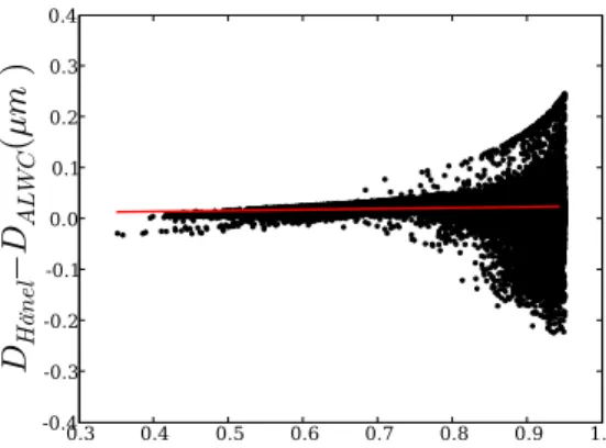
Figure2shows the differences between the wet diameter obtained with H ¨anel formula 20

(11)

ACPD

8, 1321–1365, 2008

M. Tombette et al.

Title Page

Tables Figures

◭ ◮

Back Close

Full Screen / Esc

EGU range [−0.05,0.05]µm) compared to the diameter (in average 0.35µm). At high RH,

the di_fferences could reach±0.25µm. This could be very sensitive and then the impact of such differences on AOT will be evaluated in the sensitivity study in Sect.6.

2.3.2 Wet ACRI

From Eq. (5) and from the hypothesis of a constant aerosol density, we deduce the 5

relation between the wet ACRImwet, the dry ACRImdry, CRI of water mwater and the ratio between the wet and dry diameters (also called H ¨anel’s relation):

mwet =mwater+(mdry−mwater)×

Ddry

Dwet

!3

(10)

We will also consider a computation of AOT where black carbon is a core inside a mixture composed of the other species. ACRI of the mixture will be computed with 10

Eqs. (5) and (10) and then Eq. (7) is used to compute ACRI with the black carbon core.

2.4 AOT and SSA

2.4.1 Extinction efficiency

To compute the extinction efficiencyQextfrommwetand the wet diameter of the aerosol in the bini, we use a look-up table of a Mie code at the required wavelength. The Mie 15

code used is the one fromWiscombe(1980). The look-up table provides the real part of CRI in the range [1.11–1.99] (0.01 step), the imaginary part in [0.0–0.44] (0.0043 step) and the wet diameter in [0.01–20µm] (0.2µm step).

2.4.2 Computation of the extinction coefficient

We compute the number of particles in one bin from the composition of the particles 20

(12)

ACPD

8, 1321–1365, 2008

M. Tombette et al.

Title Page

Tables Figures

◭ ◮

Back Close

Full Screen / Esc

EGU over the size bins:

bext(λ, k)=

PNbins

i=0

3×Q_ext(λ,i,k)×M_tot,i(k)×(Dwet,i(k))2

2×ρaerosol×(Ddry,i)3

(11)

whereMtot,i(z) is the total dry mass for bini.

2.4.3 AOT

Finally, we compute AOT in one given atmospheric column from Eq. (1). 5

2.4.4 SSA

The single scattering albedo used in this study (for comparisons to AERONET data) is computed as the ratio between the aerosol optical thickness due to scattering (AOT_scatt) and the total optical thickness. AOTscatt is computed in the same way as AOT, from the scattering cross section also given by the Mie code.

10

3 Instrumental set up: AERONET data

AERONET (AErosol RObotic NETwork,Holben et al.,2001) is a network constituted by more than 100 ground-based remote sensing stations providing aerosol optical, mi-crophysical, and radiative measured data. These stations are located world-wide and the network imposes standardization of instruments, calibration, processing and dis-15

tribution. This provides a basis for model-to-data comparisons at a large scale (here over Europe). It provides for each station, among other data, AOT directly measured by sun photometers and SSA retrieved from direct mesurements at different wavelengths (1020 nm, 870 nm, 675 nm and 440 nm). The data are taken from the AERONET website: http://aeronet.gsfc.nasa.gov/. The “level 2.0” data used in this study are 20

(13)

ACPD

8, 1321–1365, 2008

M. Tombette et al.

Title Page Abstract Introduction Conclusions References Tables Figures ◭ ◮ ◭ ◮ Back Close

Full Screen / Esc

EGU et al.,2001). As given inDubovik et al. (2000), we set the absolute error on SSA to

∆SSA(440)=∆SSA(675)=0.03 if AOT(440)>0.3,∆SSA(440)=∆SSA(675)=0.07 other-wise.

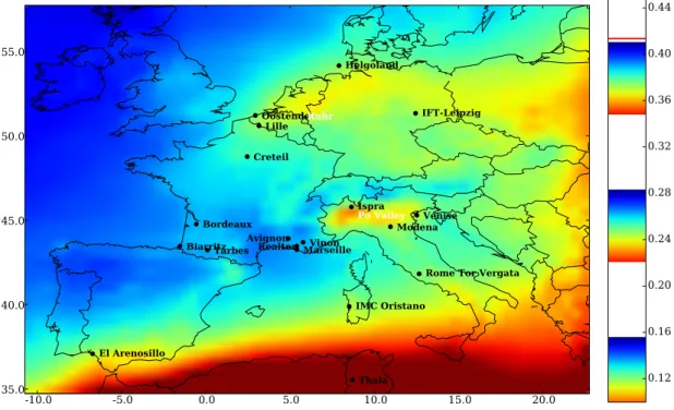
For 2001, we found out 19 stations that respect the previous conditions in our do-main. The location of the stations taken into account are plotted in Fig. 3. Here we 5

choose to compare the optical data in the mid-visible spectrum with measurements at 550 nm. SSA and AOT at 550 nm are obtained from the data at 675 and 440 nm following the Angstr ¨om law

X(550)=X(675)×

550 675

−α

(12)

whereαis the angstr ¨om exponent given by 10

α=ln X(440) X(675) /ln 675 440 , (13)

where X stands for AOT or SSA. Hamonou et al. (1999) give the relative error for computed data at 550 nm:

∆X(550) X(550) = 1₊

ln₍550₆₇₅₎ ln₍675

440) ∆X(675) X(675) +

ln₍550 675)

ln₍675₄₄₀₎

∆X(440) X(440) (14)

Raw data are instantaneous data during daylight, so hourly data are instanta-15

neous data averaged over one hour. As the asolute errors for measurements

∆AOT(440)=∆AOT(675)=0.02 is given for instantaneous data, the errors for hourly data at 550 nm are divided by the square root of the number of instantaneous data in one hour.

(14)

ACPD

8, 1321–1365, 2008

M. Tombette et al.

Title Page

Tables Figures

◭ ◮

Back Close

Full Screen / Esc

EGU

4 General configuration

Optical parameters over Europe are computed from outputs of the aerosol model SIREAM, hosted by the Chemistry-Transport Model Polair3D. SIREAM is a SIze-REsolved Aerosol Model, described in details inDebry et al.(2007). SIREAM includes 16 aerosol species: 3 primary species (mineral dust, black carbon and primary or-5

ganic), 5 inorganic species (ammonium, sulfate, nitrate, chlorure and sodium) and 8 organic species solved with the SORGAM model (Schell et al.,2001). In the usual con-figuration, SIREAM includes 5 bins logarithmically distributed over the size spectrum, that ranges from 0.01 µm to 10 µm. All these models are embedded in the POLYPHE -MUS system, available at the web adress http://www.enpc.fr/cerea/polyphemus and

10

which is described inMallet et al.(2007).

The simulation at continental scale has the same features as the simulation used for the model validation for PM₁₀ inSartelet et al.(2007). The main points are quoted hereafter.

The domain covers the area from 10.75◦W to 22.75◦E in longitude and from 34.75◦N 15

to 57.75◦N in latitude, with a step of 0.5◦. Vertically, there are five levels: 0–50 m, 50– 600 m, 600–1200 m, 1200–2000 m and 2000–3000 m. The top height of the model is considered as sufficient as a simple calculation gives that 90% of the aerosol mass is under 3 km of altitude. This calculation is made by considering that the continental aerosol is constituted by the sum of a remote concentrationc_r and a continental con-20

centrationc_c, following an exponential decrease with altitude (seeSeinfeld and Pandis, 1998, p. 445). The scale heights of those profiles are 1 km and 8 km respectively, and typical ground concentrations are taken as 1µg m−3and 45µg m−3respectively, ( War-neck,1988).

The meteorological fields are interpolated from the operational model of the Euro-25

(15)

ACPD

8, 1321–1365, 2008

M. Tombette et al.

Title Page

Tables Figures

◭ ◮

Back Close

Full Screen / Esc

EGU The boundary conditions for aerosol species are interpolated from outputs of the

GOddard Chemistry Aerosol Radiation and Transport model (GOCART, Chin et al., 2000) for the year 2001.

The anthropogenic emissions for gases and aerosols are generated from the EMEP expert inventory for 2001 (available athttp://www.emep.int).

5

Chemical species are transported through advection and diffusion. The chemical mechanism used for chemistry is RACM (Regional Atmospheric Chemistry Mecha-nism, Stockwell et al., 1997). Aerosol and gases are scavenged by dry deposition, rainout and washout. We take into account coagulation and condensation. Nucleation is not solved because the diameters of nucleated particles (typically about 1 nm) are 10

lower than the lower diameter bound of the model. Aqueous phase chemistry inside cloud droplets is also described (Variable Size Resolved Model VSRM, Fahey and Pandis,2001;Strader et al.,1998).

5 Results and discussion

We present hereafter comparisons between AERONET and simulated AOT for 2001. 15

The option taken to compute the wet diameter of the particles is the third one (with ALWC). The reason for this choice that as ALWC is solved by thermodynamics, it should be the most physical way to compute the wet diameter. Black carbon is treated as a core in the particle (non well-mixed), so we use the Maxwell-Garnett formula, with black carbon as the inclusion and the other species (including water) as the solu-20

tion. The importance of these parameters will be assessed in the sensitivity analysis in Sect.6.

5.1 Aerosol Optical Thickness

(16)

ACPD

8, 1321–1365, 2008

M. Tombette et al.

Title Page

Tables Figures

◭ ◮

Back Close

Full Screen / Esc

EGU The other regions are the Eastern Europe, the Po and the Ruhr valleys. This

corre-sponds to climatological AOT given by global models (Chin et al.,2002;Ginoux et al., 2006), or to annual AOT given inSchaap et al.(2004). The map of the latest is similar to Fig.3, but without high AOT values over North Africa because the study ofSchaap et al. (2004) did not take into account mineral dust.

5

Definition of the statistics used herafter are quoted in Table 2. Table 3 presents statistics for hourly data. These results indicate that there is a general good agreement between the simulation and observations. The mean differences between simulation and observation for hourly mean AOT range from 0.01 for Lille to 0.17 for El Arenosillo, if we except the Thala station with a very high value of 0.48. The correlations range 10

from 41.9% for Venice up to 84.9% for Biarritz. The RMSE are relatively low, in average in the vicinity of 0.2. It is noticeable that the model overestimates AOT for most of the stations (MNBE>0%), except for Biarritz station (MNBE=−34%). A reason for that overestimation could be the weak vertical discretization that leads to numerical diffusion.

15

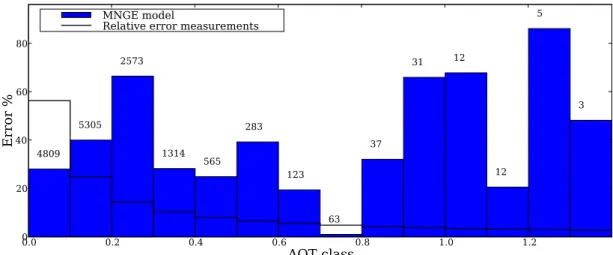
Equation (14) shows that the relative error of measurements increases with decreing AOT values. Then, the part of the model-to-observations errors that could be as-signed to the uncertainties of measurements depends on the value of AOT. To account for those uncertainties, the spectrum of AOT values for observations, ranging from 0 to 1.4, is divided into 14 classes with an interval of 0.1. Figure 4 shows the MNGE 20

between the model and the observations (blue bars), the averaged relative errors for measurements (black lines) and the number of available observations for each AOT class. For low AOT values (between 0 and 0.1), the error of the model is entirely included inside the error on measurements. For AOT between 0.1 and 0.7, a large part of the error could be attributed to the uncertainties on measurements, except for 25

(17)

ACPD

8, 1321–1365, 2008

M. Tombette et al.

Title Page

Tables Figures

◭ ◮

Back Close

Full Screen / Esc

EGU not taken into account in the model (the resuspension for example), lack of emission

sources, or errors in the transport of species are then the main sources of these dis-crepencies. These explanations are stressed by the fact that MNBE are negatives for high AOT values with a high MNGE, meaning that in these cases the model underes-timates the observations. It should be noted that MNBE is positive for the AOT class 5

1.1–1.2, with a smaller MNGE. However, the number of data in the higher AOT classes is too small to conclude for a permanent behaviour of the model.

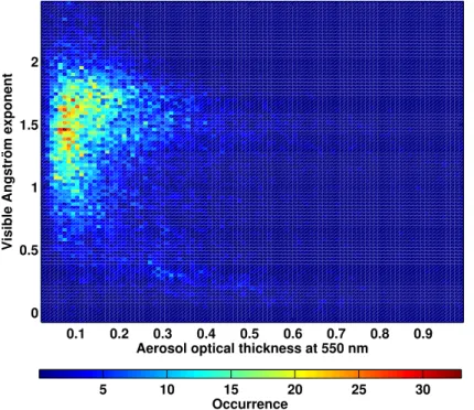
Figure 5 shows the histogram of the angstr ¨om exponent (computed from AOT at 440 and 675 nm), function of AOT at 550 nm for the observations. For small values of AOT, typically less than 0.4, where the model error is smaller than or equivalent to the 10

observation error, α>1.0 for almost all of the cases. These are pollution cases, and the model reproduces well this pollution. For high AOT values (more than 0.4), where the model error could be very large compared to the observation error, some cases whereα>1.0 present high polluted episodes, but the majority presents dust episodes (α<1.0). For AOT>0.3, 700 dust cases are listed (α<1.0) versus 150 pollution cases. 15

Figure6shows the comparison of histograms for measurements and simulation for three AERONET stations. Simulation shows good agreement for peaks, even if a shift to the right is observed (for each station), that corroborates the fact that simulation overestimates AOT. Also, these three histograms show the presence of some high values in simulated AOT that are not observed with measurements. This indicate a bad 20

computation of the concentrations and the aerosol chemical composition for specific points and times.

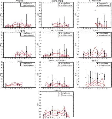
Figure 7 presents monthly time series and temporal deviation from the monthly average of AOT for observations (red crosses) and simulations (blue points) for the AERONET stations that present data for more than 5 months. These figures show 25

(18)

ACPD

8, 1321–1365, 2008

M. Tombette et al.

Title Page

Tables Figures

◭ ◮

Back Close

Full Screen / Esc

EGU sparsity of the boudary conditions for dust (monthly means for GOCART).

These results are comparable to results obtained with other models. For global model, inChin et al.(2002), AOT is overestimated at low aerosol levels, but simulated AOT agree within a factor of 2 and an overall correlation of 70% for monthly data and for all stations considered. AOT computed inGinoux et al. (2006) with global CM2.1 5

model is overestimated in polluted regions of the nothern Hemisphere by a factor of 2 when compared to AERONET data. For CTMs, Jeuken et al. (2001) find a mean difference between 0.17 and 0.19 and a spatial correlation of 68% with satellite data over Europe for the month of August 1997.Hodzic et al.(2006) reports a correlation of 61% for daily AOT at Palaiseau station for summer 2003 and inHodzic et al.(2004), the 10

RMSE between simulated and observed daily AOT ranges between 0.11 and 0.20 for every scenario considered and for the same station Palaiseau. Comparisons between daily mean AOT at 865 nm simulations over Europe and data from several AERONET stations in Hodzic et al.(2007) give RMSE ranging from 0.02 to 0.04, and NMBE of about 20%. However, these numbers are given for a small period of time (15 days in 15

August 2003).

5.2 Single Scattering Albedo

SSA, averaged over 2001, is shown in Fig.8. SSA ranges from 0.88 to 0.96. The av-eraged value over the domain is approximately 0.93. Lower values are observed over cities, as observed usually in high polluted areas (0.81 forBergin et al.,2001over Bei-20

jing, 0.8–0.88 over Mexico City forBaumgardner et al.,2000). In Paris, simulated SSA for our study lies in the range 0.88–0.90, which is coherent with the values obtained for the ESQUIF experiment (Raut and Chazette,2007b;Chazette et al.,2005). In the southeastern part of France, simulated SSA ranges here from 0.91 to 0.93, that is in the range 0.85±0.5 found inMallet et al.(2003). These low values for SSA over cities 25

(19)

ACPD

8, 1321–1365, 2008

M. Tombette et al.

Title Page

Tables Figures

◭ ◮

Back Close

Full Screen / Esc

EGU aerosols.

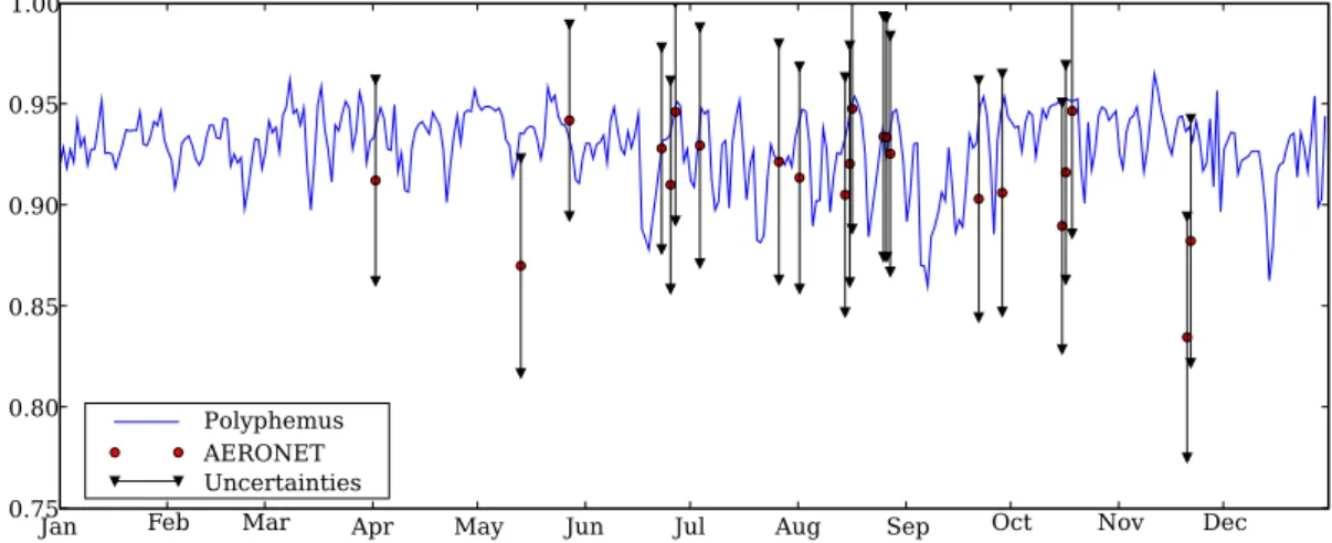
Table4shows the average of SSA retrieved from AERONET measurements and the averaged simulated SSA at the same stations and the same time. The data for SSA are too few to make further statistics, but the simulated SSA lie in the range of observations. Figure 9shows the time series of simulated SSA (blue line) and measurements (red 5

points) with the error associated to measurements computed as described in Sect.3 (black lines) for year 2001 at Ispra station. Simulation shows SSA relatively close to the observations, except for a small period in May and a majority of measurements in November where the model seems to miss events for which absorbing elements dominate the aerosol chemical composition. In spring at Ispra station, there could be 10

more coarse particles due to dust events from Sahara and more well-mixed particles that are more absorbing (Kaskaoutis et al.,2007), whereas the model considers here a core of soot for the calculation of optical properties.

6 Discussion and sensitivity study of aerosol optical properties

We present hereafter a preliminary investigation of the sensitivity with respect to the 15

calculation of the AOT, SSA and the extinction coefficients. We first define a reference

run,BC core, ref, with the following configuration (same as in Sect.5):

– the black carbon is a core;

– the other species are well-mixed with a CRI computed from Eq. (5);

– the wet diameter and water content of the aerosols are computed with output of 20

the model (from ISORROPIA, ALWC).

Then, we compare the optical parameters provided by this reference run with those simulated by alternative runs that differ with the reference run by one or two hypothesis: 1. CRI of the well-mixed envelop is computed from the Lorentz-Lorenz equation (BC

core, L-L);

(20)

ACPD

8, 1321–1365, 2008

M. Tombette et al.

Title Page

Tables Figures

◭ ◮

Back Close

Full Screen / Esc

EGU 2. the black carbon is well mixed with the other components (ALWC);

3. the black carbon is well mixed with the other components; the wet diameter is computed with the Gerber formula (Gerber);

4. the black carbon is well mixed with the other components; the liquid water content and the wet diameter are computed with the H ¨anel’s formulas (H ¨anel).

5

Tables 5, 6 and 7 report, respectively, the statistics of the fields for the AOT, the extinction coefficient and the single-scattering albedo computed with these five different versions over the whole domain and for year 2001. These fields are compared to the reference one. The RMSE between the computed AOT are lower or in the same order than those obtained for the model-to-data comparison.

10

The differences for AOT are negligeable (correlations greater than 98%), showing that this parameter is relatively stable to our hypothesis for the computation of the optical parameters. The extinction coefficients are also not really sensitive to the tested parameters. As this coefficient is given at each level of the model, this shows that the stability of the AOT is not mainly due to the vertical agregation.

15

The results for the single scattering albedo, also an agregated data in our case, are much more sensitive. Except the case were CRI of the well-mixed mixture is computed with the Lorentz-Lorenz formula (high correlation of 99%), the correlations are under 85% for the other cases. Particularly, theH ¨anel case, that is the most different one from the reference one in terms of modeling (different mixing of black carbon, different 20

computation of the aerosol water content and wet diameter) is correlated to theBC-core

run with 75%. The RMSE of the 3 casesALWC,GerberandH ¨anel, different from the reference by the mixing hypothesis, have a RMSE larger than 0.02, that is a difference of 2% between scattering and absorbing part of the aerosol. So the uncertainties lie in the absorbing component of the aerosols, that is the imaginary part of their ACRI. AOT 25

(21)

ACPD

8, 1321–1365, 2008

M. Tombette et al.

Title Page

Tables Figures

◭ ◮

Back Close

Full Screen / Esc

EGU aerosol has a great impact on the calculation of absorbing properties, the advances in

modeling the external mixing of aerosol in CTM could be of great importance. We can also guess that the way of computing the mixing state of the other species (insoluble like organics) can have an influence on the AOT, even if the effect is smaller than for black carbon. Also, the improvements in modeling the hydrophilic or hydrophobic prop-5

erties of organics and their relation to inorganics should give more precise contents for the water uptake of particles, that could have a great influence on the optical properties (see di_fferences betweenH ¨anelandALWC).

The uncertainties in computing the aerosol optical properties mainly lie in the deter-mination of the chemical composition, and then ACRI. The Chemitry Transport Models 10

contain a lot of parametrizations and numerical algorithms that result in uncertainties in the chemical composition and size distribution. It is therefore important to further investigate these uncertainties.

7 Conclusion and perspectives

We described different ways to compute the aerosol optical properties from outputs 15

of a size-resolved model. Comparisons between simulated AOT from a complex 3D size-resolved aerosol model and AERONET data have shown good agreement, when taking into account the aerosol water content computed from the inorganics composi-tion, and with the hypothesis that black carbon constitutes a core inside the particle. The stations in industrial and urban regions are fairly simulated with our model. The 20

stations influenced by dust are more badly reproduced due to boundary conditions. The simulated single scattering albedo, even in the right range in comparison with the data, could badly reproduce the observations in some particular cases. This shows the difficulties in simulating the absorbing part of the aerosol optical properties.

The hypothesis of the mixing state of the black carbon component has a great influ-25

(22)

hy-ACPD

8, 1321–1365, 2008

M. Tombette et al.

Title Page

Tables Figures

◭ ◮

Back Close

Full Screen / Esc

EGU drophylic or hydrophobic properties (Pun and Seigneur,2007). This improvement will

also be a key contribution for increasing the accuracy of simulated AOT.

Comparisons with other data will also be necessary. Satellite measurements provide a better spatial description and give an information that is similar to an average over one pixel (typically a grid cell) considered. They are therefore more representative 5

of the background aerosols than a ground-based station. Also lidar measurements will give more information about the vertical representation of aerosols and will be explored in future works. To investigate lidars at a continental scale, the EARLINET network has been created (B ¨osenberg et al., 2001). But the advantages of using such high resolution data from lidar could be fully exploited at a regional scale; the investigation 10

of the LISAIR campaign (Raut and Chazette,2007a) will be carried out in a future work. The use of a complex model has to be more deeply investigated, and a more precise sensitivity study with respect to fine physical processes has to be performed. The atmospheric optical properties also depend on the number of particles. The number distribution is nowadays not validated because of the lack of observation. Validation of 15

the number distribution simulated by models has then to be investigated. This requires short-range simulations with appropriate models (perhaps Atmospheric Computational Fluid Dynamics codes).

Acknowledgements. We thank the AERONET network for providing us freely the AOT and SSA

observations used in this study and the Principal Investigators of each site cited here. We also

20

thank the BDQA for providing us their PM₁₀ observations for year 2001. We thank also the Mozart and GOCART teams for providing us their results at global scale. One of the author, M. Tombette, is partially funded by the Ile de France region.

References

Baumgardner, D., Raga, G. B., Kok, G., Ogren, J., Rosas, I., Baez, A., and Novakov, T.: On the

25

(23)

ACPD

8, 1321–1365, 2008

M. Tombette et al.

Title Page

Tables Figures

◭ ◮

Back Close

Full Screen / Esc

EGU

Bergin, M. H., Cass, G. R., Xu, J., Fang, C., Zeng, L. M., Yu, T., Salmon, L. G., Kiang, C. S., Tang, X. Y., Zhang, Y. H., and Chameides, W. L.: Aerosol radiative, physical, and chemical properties in Beijing during June 1999, J. Geophys. Res., 106, 17 969–17 980, 2001. 1338

B ¨osenberg, J., Ansmann, A., Aldasano, J. M. B., Balis, D., Bockmann, C., Calpini, B., Chaikovski, A., Flamant, P., Hagard, A., Mitev, V., Papayannis, A., Pelon, J., Resendes, D.,

5

Schneider, J., Spinelli, N., Trickl, T., Vaughan, G., Visconti, G., and Wiegner, M.: EARLINET: A European Aerosol Research Lidar Network, Laser Remote Sensing of the Atmosphere, Selected Papers of the 20th International Laser Radar Conference, Vichy, France, edited by: A. Dabas, Loth, C., and Pelon, J., 155–158, 2001. 1342

Boucher, O. and Anderson, T. H.: General circulation model assessment of the sensitivity of

10

direct climate forcing by anthropogenic sulfate aerosols to aerosol size and chemistry, J. Geophys. Res., 100, 26 117–26 134, 1995.1324

Boutahar, J., Lacour, S., Mallet, V., Quelo, D., Roustan, Y., and Sportisse, B.: Development and validation of a fully modular platform for numerical modelling of air pollution: POLAIR, Int. J. Env. and Pollution, 22(1/2), 17–28, 2004. 1324

15

Brindley, H. E. and Ignatov, A.: Retrieval of mineral aerosol optical depth and size information from Meteosat Second Generation SEVIRI solar reflectance bands, Remote Sens. Environ., 102, 344–363, 2006. 1323

Chazette, P. and Liousse, C.: A case study of optical and chemical ground apportionment for urban aerosols in Thessaloniki, Atmos. Environ., 35, 2497–2506, 2000.1330

20

Chazette, P., Randriamiarisoa, H., Sanak, J., Couvert, P., and Flamant, C.: Optical properties of urban aerosol from airborne and ground-based in situ measurements performed during the ESQUIF program, J. Geophys. Res., 110, D02206, doi:10.1029/2004JD004810, 2005.

1338

Chin, M., Rood, R., Lin, S.-J., Muller, J. F., and Thompson, A. M.: Atmospheric sulfur cycle in

25

the global model GOCART: Model description and global properties., J. Geophys. Res., 105, 24 671–24 688, 2000. 1335

Chin, M., Ginoux, P., Kinne, S., Torres, O., Holben, B. N., Duncan, B. N., Martin, R. V., Logan, J. A., Higurashi, A., and Nakajima, T.: Tropospheric aerosol optical thickness from the GO-CART model and comparisons with satellite and sun photometer measurements, J. Atmos.

30

Sci., 59, 461–483, 2002. 1323,1336,1338

(24)

ACPD

8, 1321–1365, 2008

M. Tombette et al.

Title Page

Tables Figures

◭ ◮

Back Close

Full Screen / Esc

EGU

D24207, doi:10.1029/2005JD006356, 2005. 1323

Chung, S. and Seinfeld, J.: Global distribution and forcing of carbonaceous aerosols, J. Geo-phys. Res., 107, 4407, doi:10.1029/2001JD001397, 2002. 1328

Debry, E., Fahey, K., Sartelet, K., Sportisse, B., and Tombette, M.: Technical note: A new SIze REsolved Aerosol Model, Atmos. Chem. Phys., 7, 1537–1547, 2007,

5

http://www.atmos-chem-phys.net/7/1537/2007/. 1324,1334

Deuz é, J. L., Br éon, F. M., Devaux, C., Goloub, P., Herman, M., Lafrance, B., Maignan, F., Marchand, A. Nadal, F., Perry, G., and Tanr é, D.: Remote sensing of aerosols over land surfaces from POLDER-ADEOS-1 polarized measurements, J. Geophys. Res., 106, 4913– 4926, 2001. 1323

10

Dickerson, R. R., Kondragunta, S., Stenchikov, G., Civerolo, K. L.and Doddridge, B. G., and N., H. B.: The Impact of Aerosols on Solar Ultraviolet Radiation and Photochemical Smog, Science, 278, 827–830, 1997. 1323

Dubovik, O., Smirnov, A., Holben, B. N., King, M. D., Kaufman, Y. J., Eck, T. F., and Slutsker, I.: Accuracy assessments of aerosol optical properties retrieved from AERONET Sun and

15

sky-radiance measurements, J. Geophys. Res., 105, 9791–9806, 2000. 1333

Fahey, K. M. and Pandis, S. N.: Optimizing model performance: variable size resolution in cloud chemistry modeling, Atmos. Env., 35, 4471–4478, 2001. 1335

Forster, P., Ramaswamy, V., Artaxo, P., Berntsen, T., Betts, R., Fahey, D. W., Haywood, J., Lean, J., Lowe, D. C., Myhre, G., Nganga, J., Prinn, R., Raga, G., Schulz, M., and van Dorland,

20

R.: Changes in atmospheric constituents and in radiative forcing, in: Climate Change 2007: The physical science basis. Contribution of working group I to the fourth assessment report of the intergovernmental panel on climate change, edited by: Solomon, S., Qin, D., Manning, M., Chen, Z., Marquis, M., Averyt, K. B., Tignor, M., and Miller, H. L., 2007.1322

Gerber, H.: Relative-humidity parameterization of the Navy Aerosol Model, Technical report

25

8956, Natl. Res. Lab. Washington D.C., 1985. 1324,1330

Ginoux, P., Horrowitz, L. W., Ramaswamy, V., Geogdzhayev, I. V., Holben, B. N., Stenchikov, G., and Tie, X.: Evaluation of aerosol distribution and optical depth in the Geophysical Fluid Dynamics Laboratory coupled model CM2.1 for present climate, J. Geophys. Res., 111, D22210, doi:10.1029/2005JD006707, 2006. 1323,1336,1338

30

(25)

ACPD

8, 1321–1365, 2008

M. Tombette et al.

Title Page

Tables Figures

◭ ◮

Back Close

Full Screen / Esc

EGU

H ¨anel, G.: The properties of atmospheric aerosols as function of the relative humidity at ther-modynamic equilibrium with the surrounding moist air, Adv. Geophys., 19, 73–188, 1976.

1324,1329

Hess, M., Koepke, P., and Schult, I.: Optical properties of aerosols and clouds: the software package OPAC, B. Am. Meteorol. Soc., 79, 831–844, 1998. 1328

5

Hodzic, A., Chepfer, H., Vautard, R., Chazette, P., Beekmann, M., Bessagnet, B., Chatenet, B., Cuesta, J., Drobinski, P., Haefflin, M., and Morille, Y. a.: Comparison of aerosol chemistry transport model simulations with lidar and Sun photometer observations at a site near Paris, J. Geophys. Res., 109, D23201, doi:10.1029/2004JD004735, 2004.1323,1338

Hodzic, A., Vautard, R., Chepfer, H., Goloub, P., Menut, L., Chazette, P., Deuz ´e, J.-L., Apituley,

10

A., and Couvert, P.: Evolution of aerosol optical thickness over Europe during the August 2003 heat wave as seen from CHIMERE model simulations and POLDER data, Atmos. Chem. Phys., 6, 1853–1864, 2006,

Hodzic, A., Madronich, S., Bohn, B., Massie, S., Menut, L., and Wiedinmyer, C.: Wildfire

par-15

ticulate matter in Europe during summer 2003: Meso-scale modeling of smoke emissions, transport and radiative effects, Atmos. Chem. Phys. Discuss., 7, 4781–4855, 2007,

http://www.atmos-chem-phys-discuss.net/7/4781/2007/. 1338

Holben, B. N., Tanr ´e, D., Smirnov, A., Eck, T. K., Slutsker, I., Abuhassan, N., Newcomb, W. W., Schafer, J. S., Chatenet, B., Lavenu, F., Kaufman, Y. J., Castle, J. V., Setzer, A., Markham,

20

B., Clark, D., Frouin, R., Halthore, R., Karneli, A., O’Neil, N. T., Pietras, C., Pinker, R. T., Vass, K., and Zibordi, G.: An emerging ground-based aerosol climatology: Aerosol optical depth from AERONET, J. Geophys. Res., 106, 12 067–12 097, 2001.1332

Houghton, J., Ding, Y., Griggs, D., Noguer, M., van der Linden, P., Dai, X., Maskell, K., Johnson, C., Meira Filho, L., Bruce, J., Lee, H., Callander, B., Haites, E., Harris, N., and Maskell, K.:

25

Climate change 2001, The scientific basis, an evaluation of the IPCC, Cambridge University Press, New York, 2001.1322

Jacobson, M. Z.: A physically-based treatment of elemental carbon optics: Implications for global direct forcing of aerosols, Geophys. Res. Let., 27, 217–220, 2000.1328

Jeuken, A., Veefkind, J. P., Dentener, F., Metzger, S., and Robles Gonz ´ales, C.: Simulation

30

of the optical depth over Europe for August 1997 and a comparison with observation, J. Geophys. Res., 106, 28 295–28 311, 2001.1323,1338

(26)

Badar-ACPD

8, 1321–1365, 2008

M. Tombette et al.

Title Page

Tables Figures

◭ ◮

Back Close

Full Screen / Esc

EGU

inath, K. V. S.: Aerosol climatology: on the discrimination of aerosol types over four AERONET sites, Atmos. Chem. Phys. Discuss., 7, 6357–6411, 2007,

http://www.atmos-chem-phys-discuss.net/7/6357/2007/. 1339

Katrinak, K. A., Rez, P., Perkes, P. R., and R., B. P.: Fractal geometry of carbonaceous agre-gates from an urban aerosol, Environ. Sci. Technol., 27, 539–547, 1993.1328

5

Kaufman, Y. J., Tanr ´e, D., Remer, L. A., Vermote, E. F., Chu, A., and Holben, B. N.: Operational remote sensing of tropospheric aerosol over land from EOS moderate resolution imaging spectroradiometer, J. Geophys. Res., 102, 17 051–17 067, 1997.1323

Kinne, S., Schultz, M., Textor, C., Guibert, S., Balkanski, Y., Bauer, S. E., Berntsen, T., Berglen, T. F., Boucher, O., Chin, M., Collins, W., Dentener, F., Diehl, T., Easter, R., Feichetr, J.,

10

Fillmore, D., Ghan, S., Ginoux, P., Gong, S., Grini, A., Hendricks, J., Herzog, M., Horowitz, L., Isaken, I., Iversen, T., Kirkevag, A., Kloster, S., Koch, D. an Kristjansson, J. E., Krol, M., Lauer, A., Lamarque, J. F., Lesins, G., Liu, X., Lohmann, U., Montanaro, V., Myhre, G., Penner, J. E., Pitari, G., Reddy, S., Seland, O., Stier, P., Takemura, T., and Tie, X. a.: An AeroCom initial assessment - Optical properties in aerosol component modules of global

15

models, Atmos. Chem. Phys., 6, 1815–1834, 2006,

http://www.atmos-chem-phys.net/6/1815/2006/. 1323

Koh, G.: Effective dieclectric constant of a medium with sperical inclusions, Ieee transactions on Geosciences and Remote Sensing, 30, 184–186, 1992. 1329

Lesins, G., Chylek, P., and Lohmann, U.: A study of internal and external mixing scenarios and

20

its effect on aerosol optical properties and direct radiative forcing, J. Geophys. Res., 107, 4094–4106, 2002. 1328

Lohmann, U. and Feichter, J.: Global indirect aerosol effects: a review, Atmos. Chem. Phys., 5, 715–737, 2005,

25

Lorentz, L.: ¨Uber die Refraktionkonstanten, Annalen des Physikalische Chemie, 11, 70–103, 1880. 1327

Lorenz, H. A.: ¨Uber die Beziehung zwischen der Frotpflanzungeschwigkeit des Lichtes und der Korperdichte, Annalen des Physikalische Chemie, 9, 641–545, 1880.1327

Mallet, M., Roger, J., Despiau, S., Dubovik, O., and Putaud, J.: Microphysical and optical

30

properties of aerosol particles in urban zone during ESCOMPTE, Atmos. Res., 69, 73–97, 2003. 1338

(27)

ACPD

8, 1321–1365, 2008

M. Tombette et al.

Title Page

Tables Figures

◭ ◮

Back Close

Full Screen / Esc

EGU

Roustan, Y., Sartelet, K., Tombette, M., and Foudhil, H.: Technical Note: The air quality modeling system Polyphemus, Atmos. Chem. Phys., 7, 5479–5487, 2007,

http://www.atmos-chem-phys.net/7/5479/2007/. 1322,1324,1334

Maxwell-Garnett, J. C.: Colours in Metal Glasses and in Metallic Films, Philos. Trans. R. Soc. London., 203, 385–420, 1904. 1328

5

McMurry, P. H. X. W., Park, K., and Ehara, K.: The Relationship between Mass and Mobility for Atmospheric Particles: A New Technique for Measuring Particle Density, Aerosol Sci. Tech., 36, 227–238, 2002.1327

Mie, G.: Beitr äge zur Optik tr über Medien, speziell kolloidaler Metall ösungen, Ann. Phys. Leipzig, 330, 377–445, 1908.1325

10

Nenes, A., Pandis, S., and Pilinis, C.: ISORROPIA: A new thermodynamic equilibrium model for multiphase multicomponent inorganic aerosols, Aquat. Geoch., 4, 123–152, 1998.1330

Penner, J. E., Chang, S. Y., Chin, M., Chuang, C. C., Feichter, J., Feng, Y., Geogdzhayev, I. V., Ginoux, P., Herzog, M., Higurashi, A., Koch, D., Land, C., Lohmann, U., Mishchenko, M., Nakajima, T., Pitari, G., Soden, B., Tegen, I., and Stowe, L.: A comparison of model- and

15

satellite-derived Aerosol Optical Depth and Reflectivity, J. Atmos. Sci., 59, 441–460, 2002.

1323

Pun, B. K. and Seigneur, C.: Investigative modeling of new pathways for secondary organic aerosol formation, Atmos. Chem. Phys., 7, 2007. 1342

Putaud, J.-P., Raes, F., Dingenen, R. V., Br ¨uggemann, E., Facchini, M. C., Decesari, S., Fuzzi,

20

S., Gehrig, R., H ¨uglin, C., Laj, P., Lorbeer, G., Maenhaut, W., Mihalopoulos, N., M ¨uller, K., Querol, X., S. Rodriguez andi, J. S., Spindler, G., ten Brink, H., rseth, K. T., and Wieden-sohler, A.: A European aerosol phenomenology - 2: Chemical characteristics of particulate matter at kerbside, urban, rural and background sites in Europe, Atmos. Environ., 38, 2579– 2595, 2004. 1329

25

Ramanathan, V., Crutzen, P. J., Lelieved, J., Mitra, A. P., Althausen, D., Anderson, J., Andreae, M. O., Cantrell, W., Cass, G. R., Chung, C. E., Clarke, A. D., Coakley, J. A., Collins, W. D., Conant, W. C., Dulac, F., Heintzenberg, J., Heymsfield, A. J., Holben, S., Howell, S., Hudson, J. ans Jayaraman, A., Kiehl, J. T., Krishnamurti, T. N., Lubin, D., McFarquhar, G., Novakov, T., Ogren, J. A., Podgorny, I. A., Prather, K., Priestley, K., Prospero, J. M., Quinn, P. K.,

30

(28)

ACPD

8, 1321–1365, 2008

M. Tombette et al.

Title Page

Tables Figures

◭ ◮

Back Close

Full Screen / Esc

EGU

Randriamiarisoa, H., Chazette, P., Couvert, P., Sanak, J., and M ´egie, G.: Relative humidity impact on aerosol parameters in a Paris suburban area, Atmos. Chem. Phys., 6, 1389– 1407, 2006,

Raut, J.-C. and Chazette, P.: Retrieval of aerosol complex refractive index from a synergy

5

between lidar, sunphotometer and in situ measurements during LISAIR campaign, Atmos. Chem. Phys. Discuss., 7, 1017–1065, 2007a. 1342

Raut, J.-C. and Chazette, P.: Vertical profiles of urban aerosol complex refractive index in the frame of ESQUIF airborne measurements, Atmos. Chem. Phys. Discuss., 7, 10 799–10 835, 2007b.1338

10

Robles Gonz ´alez, C., Schaap, M., de Leeuw, G., Builtjes, P. J. H., and van Loon, M.: Spatial variation of aerosol properties over Europe derived from satellite observations and compari-son with model calculations, Atmos. Chem. Phys., 3, 521–533, 2003,

Sartelet, K. N., Debry, E., Fahey, K. M., Roustan, Y., Tombette, M., and Sportisse, B.:

Simu-15

lation of aerosols and gas-phase species over Europe with the Polyphemus system. Part I: model-to-data comparison for 2001., Atmos. Environ., 41, 6116–6131, 2007. 1324,1334

Schaap, M., van Loon, M., ten Brink, H. M., Dentener, F. J., and Builtjes, P. J. H.: Secondary in-organic aerosol simulations for Europe with special attention to nitrate, Atmos. Chem. Phys., 4, 857–874, 2004,

20

Schell, B., Ackermann, I. J., and Haas, H.: Modeling the formation of secondary organic aerosol within a comprehensive air quality model system, J. Geophys. Res., 106, 28 275–28 293, 2001. 1334

Seinfeld, J. H. and Pandis, S. N.: Atmospheric chemistry and physics, Wiley-Interscience, 1998.

25

1323,1327,1328,1334

Sportisse, B., Debry, E., Fahey, K., Roustan, Y., Sartelet, K., and Tombette, M.: PAM project (Multiphase Air Pollution): description of the aerosol models SIREAM and MAM, Tech. Rep. 2006-08, CEREA, available athttp://www.enpc.fr/cerea/polyphemus, 2006. 1330

Stockwell, W., Kirchner, F., and Kuhn, M.: A new Mechanism for regional chemistry modeling,

30

J. Geophys. Res., 102, 25 847–25 879, 1997. 1335

(29)

ACPD

8, 1321–1365, 2008

M. Tombette et al.

Title Page

Tables Figures

◭ ◮

Back Close

Full Screen / Esc

EGU

PM modelling, Technical report, STI, 1998. 1335

Tombette, M. and Sportisse, B.: Aerosol modeling at a regional scale: Model-to-data com-parison and sensitivity analysis over Greater Paris, Atmos. Environ., 41, 6941–6950, 2007.

1324

Warneck, P.: Chemistry of the natural atmosphere, Academic Press, New York, 1988.1334

5

Wiscombe, W. J.: Improved Mie scattering algorithms, Appl. Optics, 19, 1505–1509, 1980.

1331

Yu, H., Kaufman, Y. J., Chin, M., Feingold, G., Remer, L. A., Anderson, T. L., Balkanski, Y., Bel-loin, N., Boucher, O., Christopher, S., DeCola, P., Kahn, R., Koch, D., Loeb, N., Reddy, M. S., Schultz, M., Takemura, T., and Zhou, M.: A review of measurement-based assessments of

10

the aerosol direct radiative effect and forcing, Atmos. Chem. Phys., 6, 613–666, 2006,

(30)

ACPD

8, 1321–1365, 2008

M. Tombette et al.

Title Page

Tables Figures

◭ ◮

Back Close

Full Screen / Esc

EGU

Table 1. Correspondence between POLYPHEMUS aerosol species and OPAC species. The

real (Re) and imaginary parts (Im) of CRI atλ=550 nm for each species are also given.

Model Species OPAC species Re Im

(31)

ACPD

8, 1321–1365, 2008

M. Tombette et al.

Title Page

Tables Figures

◭ ◮

Back Close

Full Screen / Esc

EGU

Table 2. Definitions of the statistics used in the study. (o_i)_i and (c_i)_i are the observed and the

modeled concentrations at time and locationi, respectively. nis the number of data.

Statistic indicator Definition

Root mean square error (RMSE)

q 1 n

Pn

i=1(ci−oi)2

Correlation

Pn

i=1(ci−c)(o¯ i−o)¯

q Pn

i=1(ci−c)¯2

q Pn

i=1(oi−o)¯2

Mean normalized bias error (MNBE)

1 n

Pn i=1

ci−oi

oi

Mean normalized gross error (MNGE)

1 n

Pn i=1

|ci−oi|

(32)

ACPD

8, 1321–1365, 2008

M. Tombette et al.

Title Page

Tables Figures

◭ ◮

Back Close

Full Screen / Esc

EGU

Table 3. Number of observations, mean value for mesurements and simulation, RMSE,

cor-relations and NMBE for hourly values of AOT at 550 nm for simulation. Period: 2001-01-01 to 2001-12-31.

Station # meas. Meas. Sim. RMSE Correl. (%) MNBE (%) (hour) Mean Mean

(33)

ACPD

8, 1321–1365, 2008

M. Tombette et al.

Title Page

Tables Figures

◭ ◮

Back Close

Full Screen / Esc

EGU

Table 4. Number of observations, mean value for mesurements and simulation, for hourly

values of SSA at 550 nm. RMSE, correlations and NMBE are not computed because of the lack of data. Period: 2001-01-01 to 2001-12-31.

Station # meas. (day) Meas. Mean Sim. Mean

(34)

ACPD

8, 1321–1365, 2008

M. Tombette et al.

Title Page

Tables Figures

◭ ◮

Back Close

Full Screen / Esc

EGU

Table 5.Sensitivity of the AOT computation. Statistical indicators computed with respect to the

reference configuration.

Version Mean Std. dev. RMSE with ref. Correl. with ref.(%)

BC core (ref.) 0.265 0.31

(35)

ACPD

8, 1321–1365, 2008

M. Tombette et al.

Title Page

Tables Figures

◭ ◮

Back Close

Full Screen / Esc

EGU

Table 6. Sensitivity of the extinction coefficient computation. Statistical indicators computed

with respect to the reference configuration.

Version Mean Std. deviation RMSE with ref. Correl. with ref.(%)

BC core 1.03×10−3 1.036×10−3

(36)

ACPD

8, 1321–1365, 2008

M. Tombette et al.

Title Page

Tables Figures

◭ ◮

Back Close

Full Screen / Esc

EGU

Table 7.Sensitivity of the single scattering albedo computation. Statistical indicators computed

with respect to the reference configuration.

Version Mean Std. dev. RMSE with ref. Correl. with ref.(%)

BC core (ref.) 0.93 0.36

(37)

ACPD

8, 1321–1365, 2008

M. Tombette et al.

Title Page

Tables Figures

◭ ◮

Back Close

Full Screen / Esc

EGU

(38)

ACPD

8, 1321–1365, 2008

M. Tombette et al.

Title Page

Tables Figures

◭ ◮

Back Close

Full Screen / Esc

EGU

0.3 0.4 0.5 0.6 0.7 0.8 0.9 1.0

Relative Humidity

-0.4 -0.3 -0.2 -0.1 0.0 0.1 0.2 0.3 0.4

l

e

n

¨

a

H

C

W

L

A

)

m

μ

(

D

−

D

Fig. 2. Di_fferences between the wet diameters of the fourth section of the model (dry