www.hydrol-earth-syst-sci.net/19/1371/2015/ doi:10.5194/hess-19-1371-2015
© Author(s) 2015. CC Attribution 3.0 License.
Quantifying sensitivity to droughts –
an experimental modeling approach
M. Staudinger1, M. Weiler2, and J. Seibert1,3
1Department of Geography, University of Zurich, Zurich, Switzerland 2Chair of Hydrology, University of Freiburg, Freiburg, Germany 3Department of Earth Sciences, Uppsala University, Uppsala, Sweden
Correspondence to:M. Staudinger ([email protected])
Received: 29 June 2014 – Published in Hydrol. Earth Syst. Sci. Discuss.: 9 July 2014 Revised: 16 February 2015 – Accepted: 23 February 2015 – Published: 12 March 2015
Abstract. Meteorological droughts like those in summer
2003 or spring 2011 in Europe are expected to become more frequent in the future. Although the spatial extent of these drought events was large, not all regions were affected in the same way. Many catchments reacted strongly to the me-teorological droughts showing low levels of streamflow and groundwater, while others hardly reacted. Also, the extent of the hydrological drought for specific catchments was differ-ent between these two historical evdiffer-ents due to differdiffer-ent initial conditions and drought propagation processes. This leads to the important question of how to detect and quantify the sen-sitivity of a catchment to meteorological droughts. To assess this question we designed hydrological model experiments using a conceptual rainfall-runoff model. Two drought sce-narios were constructed by selecting precipitation and tem-perature observations based on certain criteria: one scenario was a modest but constant progression of drying based on sorting the years of observations according to annual precip-itation amounts. The other scenario was a more extreme pro-gression of drying based on selecting months from different years, forming a year with the wettest months through to a year with the driest months. Both scenarios retained the ob-served intra-annual seasonality for the region. We evaluated the sensitivity of 24 Swiss catchments to these scenarios by analyzing the simulated discharge time series and modeled storage. Mean catchment elevation, slope and area were the main controls on the sensitivity of catchment discharge to precipitation. Generally, catchments at higher elevation and with steeper slopes appeared less sensitive to meteorological droughts than catchments at lower elevations with less steep slopes.
1 Introduction
into a hydrological drought through different mechanisms that are controlled by catchment characteristics as well as climate (Eltahir and Yeh, 1999; Peters et al., 2003; Tallak-sen and Van Lanen, 2004; Van Loon and Van Lanen, 2012): several consecutive meteorological droughts can turn into a combined and prolonged hydrological drought and they can be attenuated by the storage of a catchment. Furthermore, a time lag between meteorological, soil moisture and hy-drological droughts affects both streamflow and groundwa-ter (Van Loon and Van Lanen, 2012). In addition to a deficit in precipitation, ice and snow acting as temporary storage can also cause droughts (Van Loon et al., 2010). Observed droughts reflect the diversity of drought processes which led to varyingly strong responses to meteorological droughts in different regions and catchments. Based on the various drought-generating mechanisms, Van Loon and Van Lanen (2012) developed a general hydrological drought typology and distinguished between six different drought types that in-clude the type of precipitation and air temperature conditions preceding the drought (classical rainfall deficit drought, rain-to-snow-season drought, wet-to-dry-season drought, cold-snow-season drought, warm-cold-snow-season drought, and com-posite drought).
Previous studies looked at historical droughts and tried to link the occurrence and temporal development of a drought with climate and catchment characteristics such as topog-raphy or geology (e.g., Stahl and Demuth, 1999; Zaidman et al., 2002; Fleig et al., 2006). Stahl and Demuth (1999) found that spatial and temporal variability of streamflow drought was influenced by the geographical and topograph-ical location and the underlying geology. Periods of pro-longed streamflow drought were linked with persistent oc-currence of specific circulation patterns; however, temporal streamflow drought development could not be linked to ob-served climatic drought.
Many studies have used scenarios to estimate the impact of climate change on streamflow in general and some focus on droughts in particular (e.g., Wetherald and Manabe, 1999, 2002; Wang, 2005; Lehner et al., 2006). The usual approach is to use simulations of general circulation models or re-gional climate models (GCMs/RCMs) with plausible scenar-ios of greenhouse gas emissions to drive hydrological mod-els. However, there are large uncertainties connected to the GCM and RCM simulations and the choice of bias correction method (Teutschbein and Seibert, 2012, 2013), and the range of resulting impacts is accordingly high. Wilby and Harris (2006) used different GCMs, emission scenarios, downscal-ing techniques and hydrological model versions to assess uncertainties in climate change impacts and found that the resulting cumulative distribution functions of low flow for the river Thames were most sensitive to uncertainties in cli-mate change scenarios and downscaling. Instead of dealing with these large uncertainties, here we focus on systematic changes. Thus, scenarios that exclude the large sources of uncertainty (climate change scenarios and downscaling) are
a straightforward way to investigate the different responses of catchments to droughts.
In this study we assess how sensitive different catchments are to meteorological droughts and whether this sensitivity can be linked to a specific type of catchment, classified by catchment characteristics. We aim to answer these questions using a modeling experiment with two different scenarios of progressively drier meteorological conditions, based on ob-servations.
2 Methods and data
2.1 Data
We selected 24 Swiss catchments, which vary in area, mean catchment elevation, land cover and geology (Table 1). Only catchments with minor anthropogenic influence were se-lected, i.e., no catchments with dams, major water extractions or inflow of sewage treatment plants, to investigate the main natural underlying processes. The selected catchments have, if any, minimal glacier influence and have discharge stations of satisfactory precision during low flow. Daily discharge ob-servations were provided by FOEN (2013a). Gridded temper-ature (◦C) and precipitation (mm) data (Frei, 2013) available for Switzerland (MeteoSwiss, 2013) were averaged over each catchment and then used to force the hydrological model. The observation period for discharge data used in this study extended from 1993 to 2012, for the meteorological data from 1975 to 2012. Information about catchment area, mean catchment elevation, forested land cover, and slope were ex-tracted from the digital elevation map of Switzerland (25 m resolution).
A hydrogeological productivity number, which is a mea-sure of hydraulic conductivity and thickness of the aquifer, was derived from the hydrogeological map of Switzerland (Aviolat et al., 2004): first, features of the aquifers were clas-sified as productivity (high, variable, low, very low). Then, we assigned a numeric value between 0 and 1 to each of these productivity classes (high: 1, variable: 0.5, low: 0.1, very low: 0) and computed an area-weighted mean. In a sec-ond step we investigated the influence of the choice of the numeric values by calibrating the values of the productivity classes to maximize the correlation between area-weighted mean values and sensitivity measures (described in the fol-lowing section). The calibration was conditioned so that val-ues increased from low to high productivity.
2.2 HBV modeling experiment
Rain and snow
Snow
Snow routine
tion
Snow
Snow
Evapotranspiration
Elev
a
t
Rainfall and snowmelt
TT, CFMAX, SFCF, CWH, CFR Area
FC Soil routine
FC, LP, BETA
Recharge
Q =K SUZα
g
ht
s
SUZ
Computed Q = K1SUZ
We
ig
MAXBAS
SLZ
p runoff Q = K2SLZ
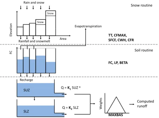
Figure 1.Structure of the HBV model.
precipitation and air temperature as well as estimates of long-term monthly potential evapotranspiration.
– Snow routine: snow accumulation and melt are com-puted by a degree-day method including snow water holding capacity and potential refreezing of meltwater.
– Soil routine: groundwater recharge and actual evapora-tion are simulated as funcevapora-tions of the actual water stor-age in the soil box. The soil moisture storstor-age is called SM.
– Response routine: runoff is computed as a function of water storage in an upper and a lower groundwater box. The groundwater storage (GW) from both groundwater boxes was summed.
– Routing routine: a triangular weighting function routes the runoff to the outlet of the catchment.
Detailed descriptions of the model can be found elsewhere (Bergström, 1995; Lindström et al., 1997; Seibert, 1999). The HBV-light model was calibrated automatically for each of the catchments over the period 1993–2012 using a ge-netic optimization algorithm with subsequent steepest gra-dient tuning (Seibert, 2000). Parameter uncertainty was ad-dressed by performing 100 calibration trials, which resulted in 100 optimized parameter sets according to a combination of Nash–Sutcliffe model efficiency and volume error (FLS, Eq. 1; Lindström et al., 1997), where the weighting factor for the latter was set to 0.1, as recommended by Lindström et al.
(1997) and Lindström (1997).FLS ranges between−∞for poor fits and 1 for a perfect fit,
FLS=1−
P
(Qobs−Qsim)2
P
Qobs−Qobs
2−0.1 P
|(Qobs−Qsim)| P
Qobs
. (1)
One simulation was run per parameter set over the entire meteorological observation period. The simulation results of this ensemble (100 selected parameter sets) were averaged at each time step to derive the reference simulation. The same was done for the scenarios. Each model simulation was pre-ceded by a 1-year warm up period.
2.3 Construction of the scenarios
We constructed two precipitation time series as purely hypo-thetical scenarios, over the period 1975–2012, with progres-sively drying conditions.
– Scenario with sorted years (SoYe): all years over the meteorological observation period were sorted from the wettest to the driest year according to the total annual precipitation. Thus, a scenario of modest but continu-ous progression of drying was derived.
pro-Table 1.Catchment characteristics (FOEN, 2013b) and calibration results; the catchments are sorted by mean catchment elevation.FLSis the model efficiency (Eq. 1).
Number River Area Mean Regime type Productivity∗ Forest RangeFLS
(km2) elevation (−) (−) (%) (−) (m a.s.l.)
1 Aach 48.5 480 pluvial 0.27 0.33 0.79–0.82
2 Ergolz 261 590 pluvial 0.37 0.41 0.84–0.86
3 Aa 55.6 638 pluvial 0.24 0.22 0.82–0.84
4 Murg 78.9 650 pluvial 0.28 0.27 0.81–0.83
5 Mentue 105 679 pluvial 0.15 0.16 0.79–0.82
6 Broye 392 710 pluvial 0.23 0.23 0.80–0.81
7 Langeten 59.9 766 pluvial 0.36 0.19 0.70–0.74
8 Rietholz 3.3 795 pluvial 0.25 0.21 0.72–0.74
9 Guerbe 117 873 pluvial 0.33 0.33 0.78–0.80
10 Biber 31.9 1009 pluvial 0.23 0.41 0.82–0.84
11 Kleine Emme 477 1050 nivo-pluvial 0.21 0.35 0.82–0.82
12 Ilfis 188 1051 nivo-pluvial 0.24 0.46 0.78–0.81
13 Sense 352 1068 pluvio-nival 0.24 0.33 0.77–0.79
14 Alp 46.6 1155 nivo-pluvial 0.23 0.45 0.76–0.78
15 Emme 124 1189 nival 0.17 0.32 0.74–0.78
16 Sitter 261 1252 nival 0.08 0.22 0.73–0.74
17 Erlenbach 0.64 1300 nivo-pluvial 0.10 0.60 0.75–0.77
18 Luempenen 0.93 1318 nivo-pluvial 0.31 0.35 0.76–0.77
19 Grande Eau 132 1560 nival 0.21 0.33 0.79–0.81
20 Schaechen 109 1717 nival 0.29 0.16 0.90–0.92
21 Allenbach 28.8 1856 nivo-glaciar 0.10 0.13 0.73–0.76
22 Riale di Calneggia 24 1996 nivo-pluvial 0.26 0.07 0.80–0.82
23 Ova da Cluozza 26.9 2368 nival 0.47 0.05 0.73–0.78
24 Dischma 43.3 2372 glacio-nival 0.21 0.02 0.77–0.81
∗Values of area-weighted catchment average assigned to hydrogeological productivity classes: not – 0; little – 0.25; variable – 0.5; productive –
1.
gression of drying in a more extreme manner than SoYe, but nevertheless keeping the natural seasonality. The daily air temperature matching the precipitation from the original time series was rearranged in parallel to the pre-cipitation scenarios; i.e., the observed temperature remained linked to the observed precipitation. For all scenarios the land cover was kept unchanged allowing one to focus on the sen-sitivity of response of streamflow by gradually drying out the catchment. The land cover also remained basically un-changed in the last 40 years in the studied catchments. These hypothetical scenarios showed the sensitivity of catchments to extreme drying conditions, particularly in relation to initial conditions (one dry year follows another). The scenarios al-low one to further include observed weather conditions com-bined with drier than ever observed initial conditions, which are still based on observed preceding precipitation.
2.4 Relative change to long-term conditions
First, we looked at the relative change of each scenario year,
xi, to the long-term mean of the reference simulation,x.
1xi=
xi
x, (2)
wherex stands for the variable of interest and i the year.
1xi was calculated for simulated runoff (Qsim), simulated
soil moisture storage (SM), and the combined simulated upper and lower groundwater storages (GW=SUZ+SLZ) (Fig. 1; Eq. 2). Secondly, to assess the catchment sensitivity to the progression of drying we calculated the interquartile range (IQR) of all1xi. IQR represents the variability during
Table 2.Spearman rank correlation coefficients between the catch-ment characteristics from Table 1. All correlations were significant at the 5 % level (Prod. no. – productivity number).
Elevation Size Slope Prod. no. Forest
Elevation 1.000 −0.362 0.853 −0.130 −0.328
Size 1.000 −0.563 −0.131 0.236
Slope 1.000 0.012 −0.108
Prod. no. 1.000 −0.244
Forest 1.000
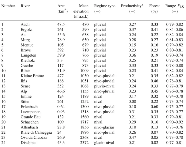
monthly precipitation differences, we accounted for the rel-ative influence of the interannual variability of precipitation in each catchment on the scenario. For each year the ratio be-tween mean annual precipitationP and long-term mean an-nual precipitationP was calculated (Fig. 2). This precipita-tion ratio was then used to account for the potential influence of the interannual precipitation variability. Each IQR was di-vided by the interquartile range of these precipitation ratios (Eq. 3) to minimize the influence of the local precipitation variability and to compare between the different catchments. The so modified IQR is referred to asIrel.
Irel=
1x75−1x25
P
P75−
P
P25
, (3)
where 1x75 is the 75th percentile of 1xi and 1x25 the 25th percentile of 1xi. Even though Irel includes both wet and dry years, it gives an overall impression of the response of a catchment to the progression of drying. We accounted for drought more specifically by comparing the extreme dry end of each scenario (driest year of both scenarios) with the long-term mean. The extreme end of each scenario was addi-tionally compared to the driest year from the reference sim-ulation in order to determine in which seasons the strongest effect of drying was found.
We looked at drought characteristics more specifically by counting the days per year that exceeded the 90th stream-flow percentile (Q90) of the respective reference simulation (100 parametrizations). Q90 is a commonly used threshold value to define hydrological drought periods. Again, we cal-culated a relative change (Eq. 2), here withxbeing the num-ber of days exceedingQ90. We used days exceedingQ90 in-stead of days below the threshold, to derive indices that are larger, when the sensitivity is higher. We used further indices that describe the influence of the progression of drying at its extreme dry end. These indices are the ratios of the differ-ence between long-term mean and mean of the driest year of each scenario and the long-term mean (1QDriest SoYefor scenario SoYe;1QDriest SoMofor scenario SoMo). As for the other indices, the larger1QDriest SoYeand1QDriest SoMoare, the more sensitive the respective catchments are to droughts. Catchment controls on the sensitivity of catchments to droughts were investigated by correlations between specific catchment characteristics (Table 1) and sensitivities using
0 5 10 15 20 25 30 35
0.5
1.0
1.5
2.0
2.5
Year
P
P
Scenario SoYe Scenario SoMo Scenario SoYe Scenario SoMo Scenario SoYe Scenario SoMo Scenario SoYe Scenario SoMo Scenario SoYe Scenario SoMo Scenario SoYe Scenario SoMo Scenario SoYe Scenario SoMo Scenario SoYe Scenario SoMo Scenario SoYe Scenario SoMo Scenario SoYe Scenario SoMo Scenario SoYe Scenario SoMo Scenario SoYe Scenario SoMo Scenario SoYe Scenario SoMo Scenario SoYe Scenario SoMo Scenario SoYe Scenario SoMo Scenario SoYe Scenario SoMo Scenario SoYe Scenario SoMo Scenario SoYe Scenario SoMo Scenario SoYe Scenario SoMo Scenario SoYe Scenario SoMo Scenario SoYe Scenario SoMo Scenario SoYe Scenario SoMo Scenario SoYe Scenario SoMo Scenario SoYe Scenario SoMo
Figure 2.Precipitation ratios of the annual precipitationsP and the
long-term mean precipitationP for scenarios SoYe and SoMo.
Spearman rank correlations. The significance of the corre-lations was evaluated using thep value of the distributions, where correlations with apvalue of<0.05 were considered significant. An important aspect in such analyses are the cor-relations among catchment characteristics themselves, which can make an interpretation of correlations between catch-ment characteristics and sensitivities more difficult. For our catchments, even though there was a significant correlation between mean catchment elevation and slope (Table 2), the highest elevation catchments do not have the steepest slopes. The influence of drier initial conditions was highlighted in a further simulation experiment based on scenario SoMo. We chose the drought in 2003 because it was one of the re-cent serious summer droughts that affected all studied catch-ments and this summer drought had a normal preceding win-ter, i.e., normal snow conditions. Recent droughts in spring (e.g., 2011, 1976) were not analyzed more specifically, as these droughts had already particularly dry initial conditions. For this simulation experiment, we used the last years of the scenario SoMo up to the end of May followed by the ac-tual series of summer 2003 starting from 1 June. In this way we simulated how much more each catchment would have been affected if the preceding months to the 2003 drought event would have been drier than actually observed. For all catchments a further index was calculated describing the sen-sitivity of the catchments to drier initial conditions and thus also to droughts by dividing the mean of the SoMo scenario-based simulation with the drier initial conditions for the sum-mer months of 2003 (June–August) by the mean of the refer-ence simulation for the same months. This index was called
1Q2003forQsim,1SM2003for SM, and1GW2003for GW. The larger these indices are, the more sensitive the respective catchments are to droughts.
sensitiv-0.0
0.5
1.0
1.5
2.0
2.5
3.0
∆
QsimScenario SoY
e
∆
SM∆
GW∆
Q90exceedance1 12 24
0 5 10 15 20 25 30 35
0.0
0.5
1.0
1.5
2.0
2.5
3.0
Year
Scenario SoMo
0 5 10 15 20 25 30 35
Year
0 5 10 15 20 25 30 35
Year
0 5 10 15 20 25 30 35
Year
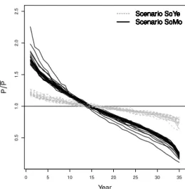
Figure 3.Relative change ofQsim, SM and GW and theQ90 exceedance days for the two scenarios to the long-term reference for all
catchments. Each color stands for one catchment number (Table 1), where the greener colors indicate catchments at the lower mean elevation and the more brownish colors were used for catchments at higher mean elevation. Note that the upper boundary of the relative change ofQ90 is given by the fixed days that are exceedingQ90per year and the maximum days per year.
ity could be attributed to snow storage. We investigated this by simulating all precipitation as rain (i.e., no snow accumu-lation) using the same parameter sets derived by the calibra-tion and repeating the scenario analyses described above.
3 Results
3.1 Interannual variation
All catchments could be calibrated satisfactorily with median
FLSvalues (Eq. 1) ranging between 0.73 and 0.92 (Table 1). The relative change of the different variables clearly indi-cated a progression of drying of streamflow as well as of the storages, where the relative change of the continuous drying for all catchments was smallest for the SM of both scenarios (Fig. 3).
The SoMo scenario generally resulted in stronger re-sponses to the drying and the relative changes specific for the different catchments became more pronounced than in scenario SoYe. During wetter conditions than the long-term mean, the1Qsim values were larger for the higher elevation
catchments compared to lower elevation catchments. During
drier conditions than the long-term mean, the1Qsim values
were smaller for the higher elevation catchments compared to lower elevation catchments. This indicates that during wet conditions the high elevation catchments were more sensi-tive to the progressive drying; however, during dry conditions high elevation catchments were less sensitive to the drying compared to lower elevation catchments. The same can also be seen for1GWwhere the change from wetter to drier con-ditions relative to the long-term GW mean shows more vari-ability between the catchments than1Qsim(Fig. 3).
DOY
274 9 59 159 259
0
5
10
15
20
Qsim [mm/da
y]
Mentue Long term mean Driest year normal Driest year (SoYe) Driest year (SoMo)
DOY
274 9 59 159 259
0
500
1000
1500
Cum
ulated Qsim [mm]
DOY
274 9 59 159 259
Ilfis
DOY
274 9 59 159 259
DOY
274 9 59 159 259
Sitter
DOY
274 9 59 159 259
DOY
274 9 59 159 259
Emme
DOY
274 9 59 159 259
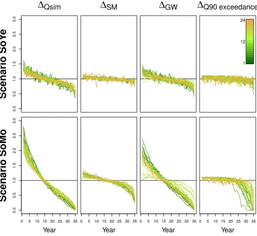
Figure 4.Qsimand cumulatedQsimfor long-term mean, driest year of the reference simulation as well as the driest years of the two scenarios
for four example catchments.
scenario SoYe (cumulative sums) confirms the variation be-tween the catchments and thus the variation in their sensitiv-ity to continuous drying (Fig. 4). The difference between the last year’s SoYe and the driest year of the reference simula-tion was minor and resulted from the different initial condi-tions caused by the preceding summer. The driest year of sce-nario SoMo resulted for each day in streamflow values below the long-term mean, the driest year of the reference simula-tion and the driest year of the SoYe scenario for all catch-ments. The discharge of the pluvial Mentue catchment was nearly 0 in the driest year of scenario SoMo. For the catch-ments with some snow influence, there remained periods of higher streamflow in spring and summer, however, with a very reduced spring flood as compared to the SoYe scenario or the reference. For the scenario SoMo, the cumulative sums show that the annual difference between long-term mean and the scenario varies among the different catchments.
3.2 Low flow frequency
The frequency of days exceeding theQ90threshold changed only little for the SoYe scenario (Fig. 3) compared to the long-term mean. Even though over the course of the years a slight decrease of days exceeding Q90 could be noticed, there were still years at the end of the scenario that had more
exceeding days than the long-term mean. For the SoMo sce-nario, however, there was a strong decrease in days exceed-ingQ90 with the progression of drying. In this scenario the difference between the catchments also became apparent: in the relatively wetter years, the lower elevation catchments al-ready started to have less days above the threshold; i.e., they were more vulnerable to droughts. In the medium dry years of the scenario, the higher elevation catchments also showed less days above the threshold compared to the long-term mean. The highest elevation catchments followed in even drier years of the scenario to show less days above the thresh-old compared to the long-term mean. In scenario SoMo, the highest elevation catchments show a clear decrease in days exceedingQ90at the dry end of the scenario.
3.3 Initial conditions
0
2
4
6
8
10
Qsim [mm/da
y]
Mentue 2003
2003 drier IC
0
50
150
SM [mm]
Jun 01 Jul 01 Aug 01
0
5
10
15
20
GW [mm]
Ilfis 2003
2003 drier IC
Jun 01 Jul 01 Aug 01
Sitter 2003
2003 drier IC
Jun 01 Jul 01 Aug 01
Emme 2003
2003 drier IC
Jun 01 Jul 01 Aug 01
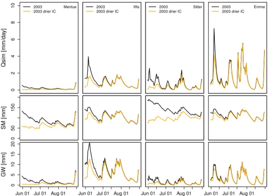
Figure 5.Simulation (median of 100 simulations) of the summer drought 2003, original and with drier initial conditions (IC).
as the simulation with drier initial conditions shows that the causes for longer or shorter influence are not the same for the different catchments: the important storage for the effect of the initial conditions for Mentue and Ilfis is composed of both storages, while for the Sitter and the Emme catchments SM seems to be stronger and more important longer than for GW.
3.4 Importance of catchment characteristics
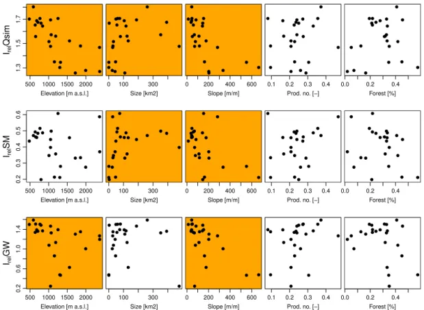
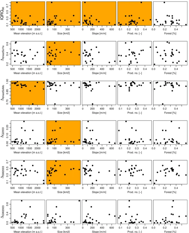
The Irel values of Qsim were significantly correlated with catchment mean elevation, size and slope, respectively (Fig. 6). Mean catchment elevation and drought sensitivity were negatively correlated, i.e., higher mean catchment ele-vations were related to lower drought sensitivities. Steeper slopes are also related to lower drought sensitivities. For SM the Irel values were significantly correlated with size and slope, while for GW the IQR values were correlated with mean catchment elevation and slope. The percentage of forested area had no significant influence on the sensitivity of the catchments to droughts, while the hydrogeological pro-ductivity numbers were only significantly correlated with the IQR of days exceeding Q90 (Fig. 6). A summary of all in-dices can be found in Table 3. The drought-targeting inin-dices (IQR of days exceeding Q90,1QDriest SoYe,1QDriest SoMo, and changes of summer 2003 with drier initial conditions
1Q2003,1SM2003 and1GW2003) could also be related to the catchment characteristics (Fig. 7); most of them were cor-related with size, elevation or slope of the catchment: IQR of days exceeding Q90 as well as 1Q2003 were significantly
correlated with size and slope of the catchment. The ratios of the driest years of the two scenarios 1QDriest SoYe and
1QDriest SoMowere significantly correlated with size and el-evation, respectively.1SM2003was correlated with mean el-evation, slope and size of the catchment.
The correlation between hydrogeology (expressed in pro-ductivity numbers) and drought sensitivity was influenced by the choice of the numeric values of the productivity classes. The correlation between hydrogeology and drought sensi-tivity could be increased from non-significant correlations to (pvalue>=0.05) Spearman rank correlation coefficients of 0.53. The correlation that existed between productivity number and days exceedingQ90 could be increased to 0.5 compared to 0.4 of the originally assigned values for each productivity class. The values for the productivity classes af-ter calibration to the different drought sensitivity indicators were high (0.79–0.97), variable (0.29–0.6), low (0.22–0.24) and very low (0.02–0.22).
3.5 Role of snow
Repeating the scenario simulations with rain instead of snow resulted in only minor changes of the sensitivities of the catchments (Fig. 8). ForIrelQsim, the higher catch-ments were slightly more sensitive to the progressive dry-ing without snow storage; however, the change in sensitiv-ity was not systematically increasing with the percentage of snow observed in the catchments. The changes inIrelGW,
● ● ● ● ●●●● ● ● ● ● ● ● ● ● ● ● ● ● ● ● ● ●
500 1000 1500 2000
1.3
1.5
1.7
Elevation [m a.s.l.] Irel
Qsim ● ● ● ● ●●●● ● ● ● ● ● ● ● ● ● ● ● ● ● ● ● ● ● ● ● ● ●●●● ● ● ● ● ● ● ● ● ● ● ● ● ● ● ● ● ● ● ● ● ● ● ● ● ● ● ● ● ● ● ● ● ● ● ● ● ● ● ● ●
0 100 300
Size [km2] ● ● ● ● ● ● ● ● ● ● ● ● ● ● ● ● ● ● ● ● ● ● ● ● ● ● ● ● ● ● ● ● ● ● ● ● ● ● ● ● ● ● ● ● ● ● ● ● ● ● ● ● ● ●● ● ● ● ● ● ● ● ● ● ● ● ● ● ● ● ● ●
0 200 400 600
Slope [m/m] ● ● ● ● ● ●● ● ● ● ● ● ● ● ● ● ● ● ● ● ● ● ● ● ● ● ● ● ● ●● ● ● ● ● ● ● ● ● ● ● ● ● ● ● ● ● ● ● ● ● ● ● ●● ● ● ● ● ● ● ● ● ● ● ● ● ● ● ● ● ●
0.1 0.2 0.3 0.4 Prod. no. [−]
● ● ● ● ● ●● ● ● ● ● ● ● ● ● ● ● ● ● ● ● ● ● ● ● ● ● ● ● ● ● ● ● ● ● ● ● ● ● ● ● ● ● ● ● ● ● ●
0.0 0.2 0.4
Forest [%] ● ● ● ● ● ● ● ● ● ● ● ● ● ● ● ● ● ● ● ● ● ● ● ● ● ●●●●● ● ● ● ● ● ● ● ● ● ● ● ● ● ● ● ● ● ●
500 1000 1500 2000
0.2
0.3
0.4
0.5
0.6
Elevation [m a.s.l.] Irel
SM ● ●●●●● ● ● ● ● ● ● ● ● ● ● ● ● ● ● ● ● ● ● ● ● ● ● ● ● ● ● ● ● ● ● ● ● ● ● ● ● ● ● ● ● ● ●
0 100 300
Size [km2] ● ● ● ● ● ● ● ● ● ● ● ● ● ● ● ● ● ● ● ● ● ● ● ● ● ● ● ● ● ● ● ● ● ● ● ● ● ● ● ● ● ● ● ● ● ● ● ● ● ●●● ● ● ● ● ● ● ● ● ● ● ● ● ● ● ● ● ● ● ● ●
0 200 400 600
Slope [m/m] ● ●●● ● ● ● ● ● ● ● ● ● ● ● ● ● ● ● ● ● ● ● ● ● ●●● ● ● ● ● ● ● ● ● ● ● ● ● ● ● ● ● ● ● ● ● ● ● ● ● ● ● ● ● ● ● ● ● ● ● ● ● ● ● ● ● ● ● ● ●
0.1 0.2 0.3 0.4 Prod. no. [−]
● ● ● ● ● ● ● ● ● ● ● ● ● ● ● ● ● ● ● ● ● ● ● ● ● ● ● ● ● ● ● ● ● ● ● ● ● ● ● ● ● ● ● ● ● ● ● ●
0.0 0.2 0.4
Forest [%] ● ● ● ● ● ● ● ● ● ● ● ● ● ● ● ● ● ● ● ● ● ● ● ● ● ● ● ● ●● ●● ● ● ● ● ● ● ● ● ●● ● ●● ● ● ●
500 1000 1500 2000
0.2
0.6
1.0
1.4
Elevation [m a.s.l.] Irel
GW ● ● ● ● ●● ●● ● ● ● ● ● ● ● ● ●● ● ●● ● ● ● ● ● ● ● ●● ●● ● ● ● ● ● ● ● ● ●● ● ●● ● ● ● ● ● ● ● ● ● ● ● ● ● ● ● ● ● ● ● ● ● ● ● ● ● ● ●
0 100 300
Size [km2] ● ● ● ● ● ● ● ● ● ● ● ● ● ● ● ● ● ● ● ● ● ● ● ● ● ● ● ● ● ● ● ● ● ● ● ● ● ● ● ● ● ● ● ● ● ● ● ●
0 200 400 600
Slope [m/m] ● ● ● ● ● ● ● ● ● ● ● ● ● ● ● ● ● ● ● ● ● ● ● ● ● ● ● ● ● ● ● ● ● ● ● ● ● ● ● ● ● ● ● ● ● ● ● ● ● ● ● ● ● ● ● ● ● ● ● ● ● ● ● ● ● ● ● ● ● ● ● ●
0.1 0.2 0.3 0.4 Prod. no. [−]
● ● ● ● ● ● ● ● ● ● ● ● ● ● ● ● ● ● ● ● ● ● ● ● ● ● ● ● ● ● ●● ● ● ● ● ● ● ● ● ● ● ● ● ● ● ● ●
0.0 0.2 0.4
Forest [%] ● ● ● ● ● ● ●● ● ● ● ● ● ● ● ● ● ● ● ● ● ● ● ●
Figure 6.IrelforQsim, SM, and GW compared to simple catchment characteristics. The orange background indicates a significant correlation
(5 % level) between the respectiveIreland catchment characteristic. Prod. no. is the hydrogeological productivity number as introduced in Sect. 2.1.
more sensitive without snow. However, for1QDriest SoYeand
1QDriest SoMothere are very small changes in sensitivity for all catchments in both directions without obvious systematic character.
4 Discussion
4.1 Sensitivity to progressive drying
We looked at the effects of the continuous progression of drying on the different catchments and found that, in gen-eral, even modest drying led to a continuous reduction of streamflow, soil moisture and groundwater storage on the one hand and on the other hand the moderate scenario already re-vealed catchments that were more sensitive to droughts than others. With the more extreme scenario the picture became even clearer. However, for the drought’s characteristic dura-tion of days exceedingQ90, only the more extreme scenario showed a clear effect. The driest year of the moderate sce-nario showed seasons with lower than the long-term mean streamflow values, which differed for catchments with differ-ent streamflow regimes. The lower elevation catchmdiffer-ents had a long, dry summer and fall. In the higher elevation catch-ments there were again higher streamflow values in late
sum-mer, which could be explained by a filling of the storages in spring. Snowmelt water could fill the storages more than it would be possible if it was only rainfed (at least in the tem-perate humid climate of Switzerland). Other differences be-tween the catchments with nival regimes have then to be ac-counted for by different storage release characteristics. This could be confirmed by the analysis of the historical drought in the summer of 2003 compared to a scenario with drier ini-tial conditions as the storages for the different catchments contributed in different proportions to the reduced stream-flow under drier initial conditions.
The relative differences were small, but the initial condi-tions can have noticeable impacts even when looking at a whole year. The differences due to initial conditions varied between about 50 and 80 %, which is in the same order of magnitude as what might be expected due to climate change (e.g., Lettenmaier et al., 1999; Nijssen et al., 2001).
im-● ●●● ●● ● ● ● ●● ●● ●●●●● ● ● ● ● ● ●
500 1000 1500 2000
0.1
0.3
0.5
0.7
Mean elevation [m a.s.l.]
IQR Q90 ● ●●● ●● ● ● ● ●● ●● ●●●●● ● ● ● ● ● ● ● ●●● ●● ● ● ● ●● ●● ●●●●● ● ● ● ● ● ● ● ● ● ● ● ● ● ● ● ● ● ● ● ●● ● ●● ● ● ● ● ● ●
0 100 300
Size [km2] ● ● ● ● ● ● ● ● ● ● ● ● ● ●● ● ●● ● ● ● ● ● ●● ● ● ● ● ● ● ● ● ● ● ● ● ●● ● ●● ● ● ● ● ● ● ● ●●● ● ● ● ● ● ● ● ● ● ● ●● ● ● ● ● ● ● ● ●
0 200 400 600
Slope [m/m] ● ●●● ● ● ● ● ● ● ● ● ● ● ●● ● ● ● ● ● ● ● ● ● ●●● ● ● ● ● ● ● ● ● ● ● ●● ● ● ● ● ● ● ● ● ● ● ● ● ● ● ● ● ● ● ● ● ● ● ● ● ● ● ● ● ● ● ● ●
0.1 0.2 0.3 0.4 Prod. no. [−]
● ● ● ● ● ● ● ● ● ● ● ● ● ● ● ● ● ● ● ● ● ● ● ● ● ● ● ● ● ● ● ● ● ● ● ● ● ● ● ● ● ● ● ● ● ● ● ● ● ● ● ● ● ● ● ● ● ● ● ● ● ● ● ● ● ● ● ● ● ● ● ●
0.0 0.2 0.4
Forest [%] ● ● ● ● ● ● ● ● ● ● ● ● ● ● ● ● ● ● ● ● ● ● ● ● ● ● ● ● ●● ● ●● ● ● ●● ● ●● ● ● ● ● ● ● ● ●
500 1000 1500 2000
0.2
0.4
0.6
Mean elevation [m a.s.l.] ∆dri
e st S o Y e ● ● ● ● ●● ● ●● ● ● ●● ● ●● ● ● ● ● ● ● ● ● ● ● ● ● ● ● ● ● ● ● ● ● ● ● ● ● ● ● ● ● ● ● ● ●
0 100 300
Size [km2] ● ● ● ● ● ● ● ● ● ● ● ● ● ● ● ● ● ● ● ● ● ● ● ● ● ● ● ● ● ● ● ● ● ● ● ● ● ● ● ● ● ● ● ● ● ● ● ● ● ● ● ● ● ● ● ● ● ● ● ● ● ● ● ● ● ● ● ● ● ● ● ●
0 200 400 600
Slope [m/m] ● ● ● ● ● ● ● ● ● ● ● ● ● ● ● ● ● ● ● ● ● ● ● ● ● ● ● ● ● ● ● ● ● ● ● ● ● ● ● ● ● ● ● ● ● ● ● ●
0.1 0.2 0.3 0.4 Prod. no. [−]
● ● ● ● ● ● ● ● ● ● ● ● ● ● ● ● ● ● ● ● ● ● ● ● ● ● ● ● ● ● ● ● ● ● ● ● ● ● ● ● ● ● ● ● ● ● ● ●
0.0 0.2 0.4
Forest [%] ● ● ● ● ● ● ● ● ● ● ● ● ● ● ● ● ● ● ● ● ● ● ● ● ● ●●●●● ● ● ●● ● ●●●●●●● ● ● ● ● ● ●
500 1000 1500 2000
0.70
0.85
1.00
Mean elevation [m a.s.l.] ∆dri
e st S o M o ● ●●●●● ● ● ●● ● ●●●●●●● ● ● ● ● ● ● ● ●●●●● ● ● ●● ● ●●●●●●● ● ● ● ● ● ● ●● ● ● ● ● ● ● ● ● ● ● ● ●● ● ●● ● ● ● ●● ●
0 100 300
Size [km2] ●● ● ● ● ● ● ● ● ● ● ● ● ●● ● ●● ● ● ● ●● ● ● ●●●●● ● ● ● ● ● ● ●● ●● ● ● ● ● ● ● ● ●
0 200 400 600
Slope [m/m] ● ●●●●● ● ● ● ● ● ● ●● ●● ● ● ● ● ● ● ● ● ● ● ● ● ● ● ● ● ● ● ● ● ● ● ● ● ● ● ● ● ● ● ● ●
0.1 0.2 0.3 0.4 Prod. no. [−]
● ● ● ● ● ● ● ● ● ● ● ● ● ● ● ● ● ● ● ● ● ● ● ● ● ● ●●●● ● ● ● ● ● ● ● ● ● ● ● ● ● ● ● ● ● ●
0.0 0.2 0.4
Forest [%] ● ● ●●●● ● ● ● ● ● ● ● ● ● ● ● ● ● ● ● ● ● ● ● ●●● ● ● ● ●●● ● ● ● ● ● ● ●● ● ● ● ● ● ●
500 1000 1500 2000
0.00
0.10
0.20
Mean elevation [m a.s.l.] ∆Q2
0 0 3 ● ●●● ● ● ● ●●● ● ● ● ● ● ● ●● ● ● ● ● ● ● ●●● ● ● ● ● ●● ● ● ● ● ● ● ● ●● ● ● ● ● ● ●
0 100 300
Size [km2] ●●● ● ● ● ● ●● ● ● ● ● ● ● ● ●● ● ● ● ● ● ●●●● ● ● ● ● ●● ● ● ● ● ● ● ● ●● ● ● ● ● ● ● ● ●●● ● ● ● ● ● ● ● ● ● ● ● ● ● ● ● ● ● ● ● ●
0 200 400 600
Slope [m/m] ● ●●● ● ● ● ● ● ● ● ● ● ● ● ● ● ● ● ● ● ● ● ● ● ●● ● ● ● ● ● ● ● ● ● ● ● ● ● ● ● ● ● ● ● ● ●
0.1 0.2 0.3 0.4 Prod. no. [−]
● ● ● ● ● ● ● ● ● ● ● ● ● ● ● ● ● ● ● ● ● ● ● ● ● ●● ● ● ● ● ● ● ● ● ● ● ● ● ● ● ● ● ● ● ● ● ●
0.0 0.2 0.4
Forest [%] ● ● ● ● ● ● ● ● ● ● ● ● ● ● ● ● ● ● ● ● ● ● ● ● ● ●● ● ● ● ● ● ● ● ● ● ● ● ● ● ● ● ● ● ● ● ● ●
500 1000 1500 2000
0.1
0.3
0.5
0.7
Mean elevation [m a.s.l.] ∆SM
2 0 0 3 ● ●● ● ● ● ● ● ● ● ● ● ● ● ● ● ● ● ● ● ● ● ● ● ● ● ● ● ● ● ● ● ● ● ● ● ● ● ● ● ● ● ● ● ● ● ● ●
0 100 300
Size [km2] ● ● ● ● ● ● ● ● ● ● ● ● ● ● ● ● ● ● ● ● ● ● ● ● ● ● ● ● ● ● ● ● ● ● ● ● ● ● ● ● ● ● ● ● ● ● ● ● ● ●● ● ● ● ● ● ● ● ● ● ● ● ● ● ● ● ● ● ● ● ● ●
0 200 400 600
Slope [m/m] ● ●● ● ● ● ● ● ● ● ● ● ● ● ● ● ● ● ● ● ● ● ● ● ● ● ● ● ● ● ● ● ● ● ● ● ● ● ● ● ● ● ● ● ● ● ● ●
0.1 0.2 0.3 0.4 Prod. no. [−]
● ● ● ● ● ● ● ● ● ● ● ● ● ● ● ● ● ● ● ● ● ● ● ● ● ● ● ● ● ● ● ● ● ● ● ● ● ● ● ● ● ● ● ● ● ● ● ●
0.0 0.2 0.4
Forest [%] ● ● ● ● ● ● ● ● ● ● ● ● ● ● ● ● ● ● ● ● ● ● ● ● ● ● ● ●●●●●● ● ● ● ●● ● ●● ● ● ● ● ● ● ●
500 1000 1500 2000
0.0
0.4
0.8
Mean elevation [m a.s.l.] ∆GW
2 0 0 3 ● ● ● ●●●●●● ● ● ● ●● ● ●● ● ● ● ● ● ● ● ● ● ● ● ● ● ● ●● ● ● ● ● ● ● ● ●● ● ● ● ● ● ●
0 100 300
Size [km2] ● ● ● ● ● ● ● ●● ● ● ● ● ● ● ● ●● ● ● ● ● ● ● ● ● ● ● ● ●●● ●● ● ● ● ● ● ● ● ● ● ● ● ● ● ●
0 200 400 600
Slope [m/m] ● ● ● ● ● ●●● ●● ● ● ● ● ● ● ● ● ● ● ● ● ● ● ● ● ● ● ● ●●● ●● ● ● ● ● ● ●● ● ● ● ● ● ● ●
0.1 0.2 0.3 0.4 Prod. no. [−]
● ● ● ● ● ●●● ●● ● ● ● ● ● ●● ● ● ● ● ● ● ● ● ● ● ● ● ● ● ● ● ● ● ● ● ● ● ● ● ● ● ● ● ● ● ●
0.0 0.2 0.4
Forest [%] ● ● ● ● ● ● ● ● ● ● ● ● ● ● ● ● ● ● ● ● ● ● ● ●
Figure 7.Indicators to drought sensitivity: days above the thresholdQ90,1QDriest SoYe,1QDriest SoMo, and changes of summer 2003 with
drier initial conditions1Q2003,1SM2003and1GW2003compared to simple catchment characteristics. The orange background indicates a significant correlation (5 % level) between the respective indicator and catchment characteristic. Prod. no. is the hydrogeological productivity number as introduced in Sect. 2.1.
proved low flow, regional regression models. However, while size was an important predictor for almost every region they investigated, elevation improved low flow prediction only in a few regions of the US. For soil moisture storage only size and slope control drought sensitivity and for groundwa-ter storage only elevation and slope control drought sensitiv-ity. Streamflow showed all the controls of the storages. The
Table 3.Drought indicators for all catchments. The smaller the value the less sensitive the catchment is to drying.
Catchment IrelQsim Irel SM Irel GW IQRQ90 1Q2003 1SM2003 1GW2003 1Qdriest SoYe 1Qdriest SoMo
Aach 1.701 0.436 1.499 0.154 0.024 0.511 0.025 0.719 1.282
Ergolz 1.802 0.471 1.588 0.236 0.026 0.315 0.037 0.737 1.242
Aa 1.653 0.493 1.338 0.199 0.015 0.364 0.120 0.848 1.567
Murg 1.558 0.462 1.507 0.207 0.028 0.497 0.031 1.383 1.985
Mentue 1.772 0.521 1.487 0.373 0.038 0.354 0.047 0.972 1.311
Broye 1.675 0.485 1.360 0.386 0.021 0.495 0.036 1.362 1.709
Langeten 1.706 0.515 1.503 0.803 0.058 0.451 0.071 1.290 1.765
Rietholz 1.668 0.198 1.483 0.207 0.001 0.281 0.001 1.934 2.527
Guerbe 1.644 0.488 1.369 0.309 0.025 0.444 0.031 1.419 1.970
Biber 1.516 0.347 1.077 0.143 0.009 0.348 0.018 2.257 2.998
Kleine Emme 1.477 0.397 0.245 0.178 0.049 0.469 0.919 2.195 2.727
Ilfis 1.695 0.446 1.465 0.240 0.198 0.583 0.283 1.915 2.424
Sense 1.572 0.498 1.328 0.208 0.027 0.478 0.046 1.619 2.128
Alp 1.350 0.213 0.861 0.117 0.004 0.290 0.010 3.544 4.233
Emme 1.561 0.357 1.133 0.113 0.325 0.728 0.432 2.439 3.025
Sitter 1.706 0.608 1.392 0.154 0.173 0.489 0.230 0.499 1.078
Erlenbach 1.303 0.211 0.476 0.099 0.007 0.313 0.314 4.483 5.158
Luempenen 1.346 0.280 0.467 0.155 0.019 0.428 0.374 4.665 5.366
Grande Eau 1.522 0.457 0.626 0.376 0.104 0.459 0.746 2.609 2.988
Schaechen 1.417 0.382 1.181 0.146 0.008 0.364 0.010 3.108 3.694
Allenbach 1.480 0.334 1.350 0.105 0.019 0.477 0.019 3.053 3.617
Riale di Calneggia 1.279 0.275 1.005 0.193 0.008 0.416 0.020 4.636 5.191
Ova da Cluozza 1.468 0.587 1.267 0.256 0.102 0.168 0.179 1.797 2.243
Dischma 1.270 0.370 1.196 0.105 0.015 0.067 0.016 2.187 2.881
● ●
●
● ● ●● ●
●
● ●
●
●
● ●
●
●●
●
● ●
●
●
●
1.2 1.4 1.6 1.8
1.2
1.4
1.6
1.8
IrelQsim Irel
Qsim no sno
w ●
●
●
● ● ●● ●
●
● ●
●
●
● ●
●
●●
●
● ●
●
●
●
●● ●
● ●●
●
●
●
● ●
●
●
● ●
●
● ●
●
●
● ●
●
●
0.2 0.3 0.4 0.5 0.6 0.7
0.2
0.3
0.4
0.5
0.6
0.7
IrelSM Irel
SM no sno
w
●● ●
● ●●
●
●
●
● ●
●
●
● ●
●
● ●
●
●
● ●
●
●
● ●
● ● ● ● ● ●
●
●
●
●
●
● ●
●
● ●
●
● ● ●
●
●
0.5 1.0 1.5
0.5
1.0
1.5
IrelGW Irel
GW no sno
w ●
●
● ● ● ● ● ●
●
●
●
●
●
● ●
●
● ●
●
● ● ●
●
●
● ● ●●
●● ●
● ● ●●
●
●
● ●● ●●
●
● ● ●
●
●
0.0 0.2 0.4 0.6 0.8 1.0
0.0
0.2
0.4
0.6
0.8
1.0
IQR Q90
IQR Q90 no sno
w
● ● ●●
●● ●
● ● ●●
●
●
● ●● ●●
●
● ● ●
●
●
● ●
● ●
●●
●
● ●
● ●
●●
● ●
●
● ●
●
● ●
●
●
●
0.2 0.3 0.4 0.5 0.6 0.7
0.2
0.3
0.4
0.5
0.6
0.7
∆DriestSoYe ∆Dri
e
st
S
o
Y
e
no sno
w
● ●
● ●
●●
●
● ●
● ●
●●
● ●
●
● ●
●
● ●
●
●
●
● ● ● ●●● ●
●
●●
●
●●●●● ● ●
●
●
● ●
●
●
0.6 0.7 0.8 0.9 1.0
0.6
0.7
0.8
0.9
1.0
∆driestSoMo ∆dri
e
st
S
o
M
o
no sno
w
● ● ● ●●● ●
●
●●
●
●●●●● ● ●
●
●
● ●
●
●
Figure 8.Comparison of the different measures of the sensitivity to drying resulting from simulations in the natural settings and simulations
all differences between the catchments. Other explanations for the sensitivity differences with elevation such as larger groundwater storage in higher elevation catchments are indi-cated by the relationship between groundwater storage and mean catchment elevation.
Hydrogeology could be expected to be correlated to a storage-dependent drought sensitivity (Stahl and Demuth, 1999; Kroll et al., 2004); however, we could not find a clear relationship using hydrogeological productivity with assigned numerical values. It could be that the other con-trols dominated and hence secondary effects like geology or land use, which are also very diverse and show a high variability among the catchments, did not show any corre-lation. It also could be that the hydrogeological productivity number was not an appropriate measure for storage and re-lease. The additional test to calibrate the numbers assigned to each productivity class in order to find the highest correla-tion between drought sensitivity measures and the hydrogeo-logical productivity number yielded a significant correlation between hydrogeology and storage-dependent drought sen-sitivity. Hence, even with the coarse hydrogeological infor-mation on which the hydrogeological productivity number was based it is possible to establish a relationship between drought sensitivity and hydrogeology. The improvement with the calibration and the resulting values for the productivity classes are to some degree dependent on the studied catch-ments. It would be good in a next step to test this dependency with a larger group of catchments. This is an important task, as the information about hydrogeological productivity could help to better estimate the sensitivity of specific catchments to droughts.
4.2 Model uncertainties
The results that are derived from the modeling experiment contain potential sources of uncertainty, i.e., mainly the choice of this hydrological model and its associated struc-ture and parametrization. The uncertainty from the model parametrization was addressed by an ensemble approach, which generated a more robust simulation than would have been the case for single “best” parametrization. Concerning the model structure we can assume that the main indication of the results of the streamflow simulation should be simi-lar for different conceptual hydrological models, whereas we can expect some differences in the simulated storages.
4.3 Construction of the scenarios
The simulations from the scenarios clearly depended on the interannual variability of precipitation for each catchment. Hence, we removed the effect of precipitation variability in the analysis by dividing the IQR values by the interquartile range of the precipitation ratio. Following many studies that document the sensitivity of streamflow to climate and cli-mate change, Schaake (1990), Dooge (1992), and
Sankara-subramanian et al. (2001) introduced and applied the so-called streamflow elasticity, which describes the sensitivity of streamflow to precipitation. The streamflow elasticity was developed as a robust, unbiased approach that on average and over many applications might discern the true sensi-tivity of streamflow to climate (Sankarasubramanian et al., 2001). Similar to our approach, the streamflow elasticity is calculated by taking annual streamflow and precipitation into account (Sawicz et al., 2011). In our approach we ensured that the interannual variability of the weather of a catchment would not overprint other catchment properties.
The scenarios were constructed by applying sorted annual or monthly precipitation, while air temperature was not con-sidered explicitly. Null et al. (2010) concon-sidered air tempera-ture and analyzed streamflow and in particular low flow sen-sitivities to climate change by using scenarios with increased temperatures but constant precipitation for mountain catch-ments. However, the results of previous case studies con-sidering total streamflow response to changes in precipita-tion and temperature indicated that future total streamflow is more sensitive to precipitation than to temperature (Letten-maier et al., 1999; Nijssen et al., 2001).
The initial wetness was not considered for the construc-tion of the scenarios but only the annual sums of precipita-tion, i.e., there might have been a dry year with a wet end of the year. This could lead to actual drier or wetter initial conditions for the following year than expected from the an-nual sum, particularly for the SoYe scenario. We minimized this effect by using hydrological years starting on 1 October. Still, there could have been a dry summer in an otherwise relatively wet year which then serves as the initial condi-tion for the following year. However, the effect should be low compared to a start in winter with, for instance, a large snow cover at the end of an otherwise dry year.
As a next step it would be interesting to perform an analy-sis similar to the one in this study for other regions as well as to find a system of general drivers that make specific catch-ments vulnerable to droughts or not. A ranking for the differ-ent catchmdiffer-ents that could (as a starting point) help drought managers to decide which catchments are more vulnerable to droughts can easily be derived from our results. In addition to the scenarios used in this study, there is also the possibil-ity to construct scenarios that have time fractions for sorting that are in between the yearly and the monthly construction of this study, for example, scenarios using half a year, a quar-ter of a year or 2 months.
5 Conclusions
This study demonstrates that hypothetical scenarios can be used to evaluate the sensitivity of catchments to droughts. The response of streamflow as well as soil moisture and groundwater storages to a continuous progression of drying was analyzed both in general as well as focusing on drought characteristics and on one historical drought event. Our anal-ysis showed that mean catchment elevation, size and slope were the main controls on the sensitivity of the catchments to drought. The results suggest that higher elevation catchments with steeper slopes were less sensitive to droughts than lower elevation catchments with less steep slopes, which could not solely be attributed to an increased snow influence. The soil moisture storage was significantly correlated to catchment size, where we found smaller catchments to be less sensi-tive to droughts than larger catchments. We did not find a clear relationship between drought sensitivity and hydroge-ology; however, another choice of the productivity classes would lead to such a relationship. Generally, for water re-sources management it is important to look at both stream-flow sensitivity and storage sensitivity to droughts. With our model-based approach the sensitivity of both can be easily estimated. This approach can serve as a starting point for water resources managers to understand the vulnerability of their catchments.
Acknowledgements. Support from the Swiss National Research Program Sustainable Water Management (NRP 61, project DROUGHT-CH) is gratefully acknowledged. The authors thank FOEN and MeteoSwiss for providing the data used in this study. Many thanks to Tracy Ewen for improving the English of the manuscript. We thank A. F. van Loon as well as an anonymous reviewer for their valuable comments.
Edited by: S. Attinger
References
Aviolat, P., Bitterli, T., Brändli, R., Christe, R., Fracheboud, S., Frei, D., George, M., Matousek, F., and Tripet, J.-P.: Hydrological At-las of Switzerland, plate 8.6, Groundwater resources, Federal of-fice for Water and Geology, Berne, 2004.
Bergström, S.: The HBV model, in: Chapter 13, Computer Mod-els of Watershed Hydrology, edited by: Singh, V. P., Water Re-sources Publications, Highlands Ranch, Colorado, USA, 443– 476, 1995.
Bréda, N., Huc, R., Granier, A., and Dreyer, E.: Temperate forest trees and stands under severe drought: a review of ecophysiologi-cal responses, adaptation processes and long-term consequences, Ann. Forest Sci., 63, 625–644, 2006.
Burke, E. J., Brown, S. J., and Christidis, N.: Modeling the recent evolution of global drought and projections for the twenty-first century with the Hadley Centre climate model, J. Hydrometeo-rol., 7, 1113–1125, 2006.
Dooge, J. C.: Sensitivity of runoff to climate change: A Hortonian approach, B. Am. Meteorol. Soc., 73, 2013–2024, 1992. Eltahir, E. A. and Yeh, P. J.-F.: On the asymmetric response of
aquifer water level to floods and droughts in Illinois, Water Re-sour. Res., 35, 1199–1217, 1999.
Fleig, A. K., Tallaksen, L. M., Hisdal, H., and Demuth, S.: A global evaluation of streamflow drought characteristics, Hydrol. Earth Syst. Sci., 10, 535–552, doi:10.5194/hess-10-535-2006, 2006. FOEN: Federal Office for the Environment, section of hydrology,
http://www.bafu.admin.ch/hydrologie/12385/index.html?lang= en (last access: 10 December 2013), 2013a.
FOEN: Federal Office for the Environment, section of hydrol-ogy, http://www.hydrodaten.admin.ch/en/ (last access: 20 De-cember 2013), 2013b.
Frei, C.: Interpolation of temperature in a mountainous region using nonlinear profiles and non-Euclidean distances, Int. J. Climatol., 34, 1585–1605, 2013.
Kohn, I., Rosin, K., Freudiger, D., Belz, J. U., Stahl, K., and Weiler, M.: Low flow in Germany in 2011, Hydrol. Wasserwirt., 58, 4– 17, 2014.
Kroll, C., Luz, J., Allen, B., and Vogel, R. M.: Developing a water-shed characteristics database to improve low streamflow predic-tion, J. Hydrol. Eng., 9, 116–125, 2004.
Lehner, B., Döll, P., Alcamo, J., Henrichs, T., and Kaspar, F.: Esti-mating the impact of global change on flood and drought risks in Europe: a continental, integrated analysis, Climatic Change, 75, 273–299, 2006.
Lettenmaier, D. P., Wood, A. W., Palmer, R. N., Wood, E. F., and Stakhiv, E. Z.: Water resources implications of global warming: A US regional perspective, Climatic Change, 43, 537–579, 1999. Li, J., Cook, E., Chen, F., Gou, X., D’Arrigo, R., and Yuan, Y.: An extreme drought event in the central Tien Shan area in the year 1945, J. Arid Environ., 74, 1225–1231, 2010.
Lindström, G.: A simple automatic calibration routine for the HBV model, Nord. Hydrol., 28, 153–168, 1997.
Lindström, G., Johansson, B., Persson, M., Gardelin, M., and Bergström, S.: Development and test of the distributed HBV-96 hydrological model, J. Hydrol., 201, 272–288, 1997.
Miller, N. L., Bashford, K. E., and Strem, E.: Potential impacts of climate change on california hydrology, J. Am. Water Resour. Assoc., 39, 771–784, 2003.
Mishra, A. K. and Singh, V. P.: A review of drought concepts, J. Hydrol., 391, 202–216, 2010.
Nijssen, B., O’Donnell, G. M., Hamlet, A. F., and Lettenmaier, D. P.: Hydrologic sensitivity of global rivers to climate change, Climatic change, 50, 143–175, 2001.
Null, S. E., Viers, J. H., and Mount, J. F.: Hydrologic response and watershed sensitivity to climate warm-ing in California’s Sierra Nevada, PLoS One, 5, e9932, doi:10.1371/journal.pone.0009932, 2010.
Peters, E., Torfs, P., Van Lanen, H., and Bier, G.: Propagation of drought through groundwater – a new approach using linear reservoir theory, Hydrol. Process., 17, 3023–3040, 2003. Rebetez, M., Mayer, H., Dupont, O., Schindler, D., Gartner, K.,
Kropp, J. P., and Menzel, A.: Heat and drought 2003 in Europe: a climate synthesis, Ann. Forest Sci., 63, 569–577, 2006. Sankarasubramanian, A., Vogel, R. M., and Limbrunner, J. F.:
Cli-mate elasticity of streamflow in the United States, Water Resour. Res., 37, 1771–1781, 2001.
Santos, J., Corte-real, J., and Leite, S.: Atmospheric large-scale dy-namics during the 2004/2005 winter drought in portugal, Int. J. Climatol., 27, 571–586, 2007.
Sawicz, K., Wagener, T., Sivapalan, M., Troch, P. A., and Carrillo, G.: Catchment classification: empirical analysis of hydrologic similarity based on catchment function in the eastern USA, Hy-drol. Earth Syst. Sci., 15, 2895–2911, doi:10.5194/hess-15-2895-2011, 2011.
Schaake, J. C.: From climate to flow, inClimate Change and U.S. Water Resources, in: chap. 8, edited by: Waggoner, P. E., John Wiley, New York, 177–206, 1990.
Seibert, J.: Regionalisation of parameters for a conceptual rainfall-runoff model, Agr. Forest Meteorol., 98, 279–293, 1999. Seibert, J.: Multi-criteria calibration of a conceptual runoff model
using a genetic algorithm, Hydrol. Earth Syst. Sci., 4, 215–224, doi:10.5194/hess-4-215-2000, 2000.
Seibert, J. and Vis, M. J. P.: Teaching hydrological modeling with a user-friendly catchment-runoff-model software package, Hy-drol. Earth Syst. Sci., 16, 3315–3325, doi:10.5194/hess-16-3315-2012, 2012.
Solomon, S.: Climate change 2007 – the physical science basis: Working group I contribution to the fourth assessment report of the IPCC, vol. 4, Cambridge University Press, 2007.
Stahl, K. and Demuth, S.: Linking streamflow drought to the occur-rence of atmospheric circulation patterns, Hydrolog. Sci. J., 44, 467–482, 1999.
Tallaksen, L. M. and Van Lanen, H. A.: Hydrological Drought: Pro-cesses and Estimnation Methods for Streamflow and Groundwa-ter, vol. 48, Elsevier, Amsterdam, the Netherlands, 2004. Teutschbein, C. and Seibert, J.: Bias correction of regional climate
model simulations for hydrological climate-change impact stud-ies: Review and evaluation of different methods, J. Hydrol., 456, 12–29, 2012.
Teutschbein, C. and Seibert, J.: Is bias correction of re-gional climate model (RCM) simulations possible for non-stationary conditions?, Hydrol. Earth Syst. Sci., 17, 5061–5077, doi:10.5194/hess-17-5061-2013, 2013.
Trenberth, K. E., Dai, A., van der Schrier, G., Jones, P. D., Barichivich, J., Briffa, K. R., and Sheffield, J.: Global warming and changes in drought, Nat. Clim. Change, 4, 17–22, 2014. Trigo, R. M., Gouveia, C. M., and Barriopedro, D.: The intense
2007–2009 drought in the Fertile Crescent: Impacts and associ-ated atmospheric circulation, Agr. Forest Meteorol., 150, 1245– 1257, 2010.
Van Loon, A. F. and Van Lanen, H. A. J.: A process-based typol-ogy of hydrological drought, Hydrol. Earth Syst. Sci., 16, 1915– 1946, doi:10.5194/hess-16-1915-2012, 2012.
Van Loon, A. F., van Lanen, H. A., Hisdal, H., Tallaksen, L. M., Fendeková, M., Oosterwijk, J., Horvát, O., and Machlica, A.: Understanding hydrological winter drought in Europe, Global Change: Facing Risks and Threats to Water Resources, IAHS Publ., 340, 189–197, 2010.
Wang, G.: Agricultural drought in a future climate: results from 15 global climate models participating in the IPCC 4th assess-ment, Clim. Dynam., 25, 739–753, 2005.
Wetherald, R. T. and Manabe, S.: Detectability of summer dryness caused by greenhouse warming, Climatic Change, 43, 495–511, 1999.
Wetherald, R. T. and Manabe, S.: Simulation of hydrologic changes associated with global warming, J. Geophys. Res., 107, 4379, doi:10.1029/2001JD001195, 2002.
Wilby, R. L. and Harris, I.: A framework for assessing uncer-tainties in climate change impacts: Low-flow scenarios for the River Thames, UK, Water Resour. Res., 42, W02419, doi:10.1029/2005WR004065, 2006.