www.atmos-chem-phys.net/15/11501/2015/ doi:10.5194/acp-15-11501-2015
© Author(s) 2015. CC Attribution 3.0 License.
A perturbed parameter model ensemble to investigate Mt.
Pinatubo’s 1991 initial sulfur mass emission
J.-X. Sheng1,a, D. K. Weisenstein2, B.-P. Luo1, E. Rozanov1,3, F. Arfeuille4,b, and T. Peter1
1Institute for Atmospheric and Climate Science, ETH Zurich, Zurich, Switzerland 2School of Engineering and Applied Science, Harvard University, Cambridge, MA, USA
3Physikalisch-Meteorologisches Observatorium Davos and World Radiation Center, Davos, Switzerland
4Oeschger Centre for Climate Change Research and Institute of Geography, University of Bern, Bern, Switzerland anow at: School of Engineering and Applied Science, Harvard University, Cambridge, MA, USA
bnow at: Empa, Swiss Federal Laboratories for Materials Testing and Research, Dübendorf, Switzerland
Correspondence to:J.-X. Sheng ([email protected])
Received: 8 December 2014 – Published in Atmos. Chem. Phys. Discuss.: 18 February 2015 Revised: 28 September 2015 – Accepted: 30 September 2015 – Published: 19 October 2015
Abstract. We have performed more than 300 atmospheric simulations of the 1991 Pinatubo eruption using the AER 2-D sulfate aerosol model to optimize the initial sulfur mass in-jection as a function of altitude, which in previous modeling studies has often been chosen in an ad hoc manner (e.g., by applying a rectangular-shaped emission profile). Our simula-tions are generated by varying a four-parameter vertical mass distribution, which is determined by a total injection mass and a skew-normal distribution function. Our results suggest that (a) the initial mass loading of the Pinatubo eruption is approximately 14 Mt of SO2; (b) the injection vertical
dis-tribution is strongly skewed towards the lower stratosphere, leading to a peak mass sulfur injection at 18–21 km; (c) the injection magnitude and height affect early southward trans-port of the volcanic clouds as observed by SAGE II.
1 Introduction
The eruption of Mt. Pinatubo on 15 June 1991 injected large amounts of sulfur dioxide into the stratosphere. It per-turbed the radiative, dynamical and chemical processes in the Earth’s atmosphere (McCormick et al., 1995) and caused a global surface cooling of approximately 0.5 K (Dutton and Christy, 1992). The Pinatubo eruption serves as a useful ana-logue for geoengineering via injection of sulfur-containing gases into the stratosphere (Crutzen, 2006; Robock et al., 2013). Therefore, modeling volcanic eruptions advances our
knowledge not only of the eruptions themselves on weather and climate, but also potential impacts of stratospheric sul-fate geoengineering.
The uncertainties in determining the initial total mass and altitude distribution of SO2 released by Pinatubo remain
high. Stowe et al. (1992) deduced a mass of 13.6 megatons of SO2based on the aerosol optical thickness observed by
the Advanced Very High Resolution Radiometer (AVHRR). By analyzing SO2 absorption measurements from the
To-tal Ozone Mapping Spectrometer (TOMS) satellite instru-ment, Bluth et al. (1992) estimated an initial mass loading of approximately 20 Mt of SO2. This study was later
reeval-uated by Krueger et al. (1995), who determined a range of 14–28 Mt emitted by Pinatubo, given the large retrieval un-certainties associated with TOMS. Later, Guo et al. (2004) constrained this range to 14–22 Mt of SO2. Besides the
to-tal emitted mass, the altitude distribution of the SO2
emis-sion is also not well constrained. The only available measure-ments with vertical resolution of SO2in the stratosphere
very different mass loadings, emission altitudes and vertical mass distributions, which leads to biases in the local heating and consequently in the dynamical response and time evolu-tion of the stratospheric aerosol burden. These uncertainties, in addition to model-specific artifacts, make it difficult to ac-curately simulate the Pinatubo eruption.
Here, we attempt to provide a solution to the problems out-lined above. We use the AER 2-D size-bin resolving (also called sectional or spectral) sulfate aerosol model (Weisen-stein et al., 1997), which participated in an international aerosol assessment (SPARC, 2006), and was one of the best-performing stratospheric aerosol models (in terms of com-paring SO2, aerosol size distributions and extinctions with
observations) under both background and volcanic condi-tions. We present results from more than 300 atmospheric simulations of the Pinatubo eruption based on different com-binations of four emission parameters, namely the total SO2
mass and a three-parameter skew-normal distribution of SO2
as a function of altitude. We calculate aerosol extinctions from all of the simulations and compare them with Strato-spheric Aerosol and Gas Experiment II (SAGE II) measure-ments (Thomason et al., 1997, 2008). Such a head-on ap-proach is currently impossible for global 3-D models due to computational expenses. The purpose of this work is to pro-vide a universal emission scenario for global 3-D model sim-ulations. To this end, we optimize the emission parameters such that the resulting SO2plume, aerosol size distributions,
aerosol burdens and extinctions match balloon-borne, satel-lite and lidar measurements. We repeat two simulations us-ing the 3-D SOCOL-AER aerosol–chemistry–climate model (Sheng et al., 2015) as a consistency check in a more complex model. In Sect. 2 we describe the model and the experimental design of our Pinatubo simulations. Section 3 compares the Pinatubo simulations with the observations, and conclusions follow in Sect. 4.
2 Method
2.1 AER 2-D sulfate aerosol model
The AER 2-D sulfate aerosol model participated in an in-ternational aerosol assessment (SPARC, 2006), in which it was compared with satellite, ground lidar and balloon mea-surements, as well as with other 2-D and 3-D aerosol mod-els, and subsequently recognized as one of the best existing stratospheric aerosol models with respect to SO2, aerosol
size distributions and extinctions under both background and volcanic conditions. The model represents sulfuric acid aerosols (H2SO4/H2O) on the global domain from the
sur-face to about 60 km with approximately 9.5◦horizontal and 1.2 km vertical resolution. The model is driven by year-by-year wind fields and temperature from Fleming et al. (1999), which were derived from observed ozone, water va-por, zonal wind, temperature, planetary waves, and
quasi-biennial oscillation (QBO). The model chemistry includes the sulfate precursor gases carbonyl sulfide (OCS), sulfur dioxide (SO2), sulfur trioxide (SO3), sulfuric acid (H2SO4),
dimethyl sulfide (DMS), carbon disulfide (CS2), hydrogen
sulfide (H2S) and methyl sulfonic acid (MSA). The model
uses pre-calculated values of OH and other oxidants from Notholt et al. (2005). Photodissociation and chemical reac-tions are listed in Weisenstein et al. (1997) and their rates are updated to Sander et al. (2011). The particle distribu-tion is resolved by 40 size bins spanning wet radii from 0.39 nm to 3.2 µm by volume doubling. Such a sectional approach was proven to be more accurate in representing aerosol mass/extinctions compared to prescribed unimodal or multimodal lognormal distributions (Weisenstein et al., 2007). The sulfuric acid aerosols are treated as liquid bi-nary solution droplets. Their exact composition is directly derived from the surrounding temperature and humidity ac-cording to Tabazadeh et al. (1997). Microphysical processes in the model include homogeneous nucleation, condensa-tion/evaporation, coagulation, sedimentation, as well as tro-pospheric rainout/washout. These processes determine the evolution of the aerosol concentration in each size bin and thereby the entire particle size distribution. Operator split-ting methods are used in the model with a time step of 1 hour for transport, chemistry, and microphysics, and 3 min sub-steps for the microphysical processes that exchange gas-phase H2SO4 with condensed phase, and 15 min sub-steps
for the coagulation process. For more detailed descriptions of chemistry and microphysics in the model we refer to Weisen-stein et al. (1997, 2007).
2.3 Experiments
We have simulated the Pinatubo-like eruption by injecting SO2 directly into the stratosphere. In the 2-D model, the
injection is immediately mixed zonally, and takes place in the latitude band 5◦S–14◦N, which is an approximation to the observed rapid zonal transport of the SO2cloud derived
from satellite measurements (Bluth et al., 1992; Guo et al., 2004). The lack of zonal resolution is clearly a deficiency of our approach, but since SO2 removal/conversion rate
(e-folding time) is sufficiently slow (τ ∼25 days) and the zonal transport around the globe sufficiently fast (τ ∼20 days) (Guo et al., 2004), a zonal-mean description is a reason-able approximation. Also, the spaceborne aerosol data are typically provided as zonal averages. We examined three cases of total mass, namely 14, 17 and 20 Mt of SO2. The
injection height extends from near the tropical tropopause (17 km) to 30 km. The vertical mass distribution is then rep-resented byMtotF (z)whereMtotis the SO2mass magnitude
in units of megaton (Mt) andF (z)=f (z)/Rzzmax=30
min=17f (x)dx
(in km−1) is a vertical distribution function of altitudez∈ [17 km, 30 km]with a skew-normal distributionf (z)given by (Azzalini, 2005)
f (z)=√2
2π σe
−(z−2σµ)22 αZz−σµ
−∞
1
√
2πe
−x22 dx.
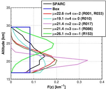
Figure 1 shows a few examples ofF (z). The location pa-rameterµdepends on available model levels and determines the altitude where the maximum of the emitted SO2cloud is
located when there is no skewness. The skewness or asym-metry of the curve increases when|α|increases and vanishes when α=0 (normal distribution). A negative α drives the location of the maximum SO2 emission to lower altitudes,
while a positive α to higher altitudes. The scale parameter
σ indicates how much dispersion takes place near the maxi-mum; that is, it determines the width or standard deviation of the asymmetric bell-shaped curve.
The four parameters Mtot, µ, σ andα enable
represen-tation of a substantial space of SO2 distributions, whose
evolution is computed forward in time (taking into account the transport and comprehensive chemical and microphysi-cal processes), in order to compare with satellite and in situ data. We simulate the following cases in detail:
Mtot∈ {14 Mt, 17 Mt,20 Mt},
µ∈ {16.79 km+n×1.16 km, n=0. . .11}, σ ∈ {2 km,3 km,4 km},
α∈ {−2,−1,0},
which results in 324 different scenarios. The choice of the boundaries for this set of scenarios is already based on ex-ploratory simulations. For example, based on the results of our 2-D model, it does not make sense to consider total
0 0.1 0.2 0.3 0.4
15 20 25 30 35
F(z) [km−1]
Altitude [km]
SPARC Box
µ=22.6 σ=4 α=−2 (R001, R033)
µ=19.1 σ=4 α= 0 (R010) µ=21.4 σ=2 α=−2 (R017)
µ=21.4 σ=3 α=−1 (R086)
µ=26.1 σ=3 α=−1 (R153)
Figure 1.Vertical distribution functionF (z). Black line: used in
SPARC (2006). Blue line: uniform (box) profile that distributes SO2
homogeneously with altitudes. Each of these curves encloses a unit area.
massesMtot>20 Mt, since no choice of the other three
pa-rameters would allow to reconcile the model results with the observations. Similarly, skewness α >0 leads to more biased model results, because the skew towards higher alti-tudes cannot be offset by lowerMtot. In addition to the above
324 simulations, we consider another two scenarios, which are adopted in modeling studies of Pinatubo: (1) Box14Mt has a uniform (“Box”) profile, which is similar to Dhomse et al. (2014) and the simulation “CONTROL_HIGH” in Aquila et al. (2012), injecting the SO2mass homogeneously
along altitudes (shown in Fig. 1); (2) SPARC20Mt is the re-production of the Pinatubo simulation conducted in SPARC (2006), which injects 20 Mt of SO2and has a vertical profile
“SPARC” shown in Fig. 1.
A selected list from the 326 2-D simulations is summa-rized in Table 1, in which the specific choice of the four pa-rameters for each scenario is provided. The score and ranking of these scenarios are discussed later in the text.
Given the limitation of the 2-D approach, we further per-form two 3-D Pinatubo-like simulations (R001 3-D and R153 3-D at the bottom of Table 1) using the coupled aerosol– chemistry–climate model SOCOL-AER Sheng et al. (2015) to check the consistency between 2-D and 3-D approaches. Note that the location parameters used in the 3-D runs dif-fer slightly from the corresponding 2-D runs (i.e., R001 and R153) due to different vertical model levels between the two models.
3 Results and discussions
We compare our results with SO2vertical profiles measured
Up-Table 1.Scores and rankings of 326 AER 2-D atmospheric simulations of the Pinatubo eruption sorted according to the weighted rank
(“RankWt”). The weighting is given by 16.7 % of the SO2score (ScoreSO2), 16.7 % of the OPC score (ScoreOPC), 33.3 % of the global
burden score (ScoreBurden), and 33.3 % of the aerosol extinction score (ScoreExt). The rank computed by the arithmetic average of the four scores is also provided (“RankAvg”). Scores of two additional 3-D simulations “R001 3-D” and “R153 3-D” from the aerosol–chemistry– climate model SOCOL-AER are provided at the bottom of the table.
Mass Location Scale Skewness Score Score Score Score Score Score Rank Rank Rank Rank Rank Rank Scenario
(Mt SO2) µ(km) σ(km) α SO2 OPC Burden Ext Avg Wt SO2 OPC Burden Ext Avg Wt Name
14 22.59 4 −2 0.22 0.47 0.16 0.22 0.27 0.24 20 23 7 10 2 1 R001
14 22.59 3 −2 0.11 0.47 0.19 0.25 0.26 0.25 4 24 14 30 1 2
14 20.27 2 0 0.19 0.47 0.19 0.24 0.27 0.25 14 21 11 25 3 3
14 21.43 3 −1 0.28 0.47 0.17 0.22 0.28 0.25 29 22 8 11 5 4
14 21.43 4 −1 0.35 0.50 0.14 0.20 0.30 0.25 52 46 2 3 7 5
14 19.11 3 0 0.38 0.48 0.15 0.20 0.30 0.26 57 32 4 5 8 6
14 21.43 2 −1 0.19 0.45 0.21 0.26 0.28 0.26 13 13 19 33 4 7
14 17.95 4 0 0.44 0.50 0.13 0.19 0.32 0.26 72 49 1 2 15 8 R008
14 20.27 3 0 0.31 0.53 0.17 0.21 0.30 0.27 42 67 9 7 9 9
14 19.11 4 0 0.41 0.54 0.14 0.19 0.32 0.27 68 77 3 1 18 10 R010
14 22.59 3 −1 0.22 0.52 0.21 0.24 0.30 0.27 18 65 20 20 6 11
14 20.27 4 −1 0.45 0.46 0.16 0.21 0.32 0.28 77 17 6 9 22 12
14 21.43 4 −2 0.40 0.45 0.19 0.23 0.32 0.28 64 8 12 14 16 13
14 22.59 4 −1 0.34 0.54 0.19 0.21 0.32 0.28 51 88 13 8 19 14
14 16.79 4 0 0.50 0.48 0.15 0.20 0.33 0.28 88 29 5 4 26 15
14 21.43 3 −2 0.37 0.44 0.21 0.24 0.31 0.28 54 3 18 28 14 16
14 21.43 2 −2 0.28 0.43 0.24 0.27 0.31 0.29 31 1 28 53 10 17 R017
14 23.75 4 −2 0.29 0.54 0.22 0.24 0.32 0.29 36 81 24 18 21 18
14 21.43 2 0 0.20 0.53 0.25 0.27 0.31 0.29 16 69 35 46 11 19
14 17.95 3 0 0.51 0.46 0.18 0.22 0.34 0.30 89 16 10 13 32 20
... ... ...
14 22.59 2 −2 0.34 0.47 0.23 0.29 0.33 0.31 49 20 26 72 27 32
17 22.59 4 −2 0.07 0.55 0.31 0.32 0.31 0.31 3 96 63 103 13 33 R033
17 21.43 4 −1 0.23 0.57 0.28 0.27 0.34 0.32 23 105 48 50 29 34
... ... ...
17 22.59 3 −1 0.21 0.60 0.40 0.38 0.40 0.40 17 126 124 151 66 84
14 22.59 2 0 0.54 0.60 0.34 0.29 0.44 0.40 95 120 81 73 91 85
20 21.43 3 −1 0.04 0.62 0.44 0.45 0.39 0.40 1 142 154 180 58 86 R086
17 23.75 4 −2 0.30 0.62 0.42 0.39 0.43 0.42 39 140 138 155 86 99
20 19.11 4 −2 0.71 0.52 0.36 0.30 0.47 0.42 135 62 96 86 105 100
14 / / / 0.70 0.70 0.31 0.26 0.49 0.43 133 184 66 36 119 101 Box14Mt
17 17.95 3 −1 0.77 0.49 0.34 0.32 0.48 0.43 151 38 82 100 110 102
... ... ...
14 26.07 3 −1 0.94 0.71 0.43 0.32 0.60 0.53 197 195 141 104 167 153 R153
... ... ...
17 16.79 3 −2 0.96 0.61 0.55 0.54 0.67 0.63 204 138 204 224 200 213
20 / / / 0.47 0.78 0.67 0.59 0.63 0.63 79 244 249 241 178 214 SPARC20Mt
20 21.43 3 0 0.48 0.75 0.66 0.62 0.63 0.63 82 220 242 251 177 215
... ... ...
20 29.55 3 −1 1.46 0.92 0.92 0.95 1.06 1.02 307 310 313 320 320 322
20 28.39 3 0 1.42 0.93 0.93 0.96 1.06 1.02 301 312 315 324 319 323
20 28.39 2 0 1.60 0.88 0.89 0.94 1.08 1.02 320 298 298 317 322 324
20 29.55 2 −1 1.67 0.86 0.88 0.93 1.08 1.02 321 288 297 313 326 325
20 29.55 3 0 1.52 0.90 0.91 0.95 1.07 1.02 317 306 306 322 321 326
14 ∼22 4 −2 0.30 0.46 0.18 0.20 0.29 0.25 R001 3-D
14 ∼26 3 −1 0.93 0.53 0.36 0.38 0.55 0.49 R153 3-D
per Atmosphere Research Satellite (UARS) between 10◦S– 0◦latitudes in September 1991 (Read et al., 1993), the
op-tical particle counter (OPC) measurements operated above Laramie, Wyoming (Deshler et al., 2003; Deshler, 2008), the global aerosol burden derived from the High-resolution In-frared Radiation Sounder (HIRS) (Baran and Foot, 1994) and from Stratospheric Aerosol and Gas Experiment II (SAGE II) using the 4λmethod (SAGE-4λ) (Arfeuille et al., 2013; Luo, 2015), as well as aerosol extinctions measured by SAGE II (Thomason et al., 1997, 2008).
3.1 Metrics and data sets
To determine an optimal set of the emission parameters, we define four metrics (ScoreSO2, ScoreBurden, ScoreOPC and
ScoreExt) based on these four measurements sets described above, and rank all of our 326 simulations by a weighted score (ScoreWt) of the four metrics (see Table 1).
ScoreSO2is calculated as the relativel2-norm (Euclidean
norm) error with respect to the MLS measurements:
whereXis a 1-D vector of SO2mixing ratio in altitude (21,
26, 31, 36 and 41 km). The negative values of the MLS mea-surements are set to zero in the calculation.
ScoreBurdenis the average of the relativel2-norm errors with respect to HIRS (July–December 1991) and SAGE-4λ
(January 1992–December 1993): 1
2(||B
t1 model−B
t1
HIRS||/||B t1 HIRS||
+ ||Bt2 model−B
t2
SAGE||/||B t2 SAGE||),
where Bt1 is a 1-D (in time) vector of the aerosol
bur-den for July–December 1991 and Bt2 for January 1992–
December 1993.
ScoreOPC– We first calculate the relativel2-norm errors with respect to the OPC measurements:
errOPC= ||Nmodel−NOPC||/||NOPC||,
where N is a 1-D vector of the cumulative particle num-ber concentration in altitude (15–30 km). We then evaluate a quadratic mean (RMS):
rmsOPC=RMS{errOPCr},
where r denotes four particle size channels (r >0.01 µm,
r >0.15 µm, r >0.25 µm and r >0.5 µm). Finally, Score-OPC is obtained by averaging rmsScore-OPC from October 1991 to December 1992.
ScoreExt – The uncertainty of SAGE is generally bet-ter than ∼20 % for 525 nm and∼10 % for 1020 nm (see Fig. 4.1 in SPARC, 2006). Therefore, ScoreExt is weighted as one-third for 525 nm (ScoreExt525nm) and two thirds for 1020 nm (ScoreExt1020nm). We use the SAGE II observa-tions between 18 and 30 km. The calculaobserva-tions for Score-Ext525nm and ScoreExt1020nm are similar to those in ScoreOPC. Latitude bands (50–40◦S, 30–20◦S, 5◦S–5◦N, 20–30◦N and 40–50◦N) take the place of the particle size channels. The temporal average is from January 1992 to De-cember 1993.
Note that extinction coefficients in the lower stratosphere (18–23 km) have a much larger weight than those above 23 km because extinctions at 525 nm and 1020 nm at 18– 23 km after the Pinatubo eruption (see Fig. 5) are one to sev-eral orders of magnitude larger than those above 23 km. We calculate the score by the relative Euclidean norm, therefore the scores above 23 km have a relatively small weight.
The overall score ScoreWt is weighted as follows: 16.7 % of the SO2 score (ScoreSO2), 16.7 % of the OPC score
(ScoreOPC), 33.3 % of the global burden score (ScoreBur-den), and 33.3 % of the aerosol extinction score (ScoreExt). The choice of the weighting is discussed below.
MLS detected residual SO2 in the stratosphere
approx-imately 100 days after the eruption. The uncertainty of ScoreSO2 is likely larger than ScoreBurden and ScoreExt
due to uncertain OH fields. An assumed uncertainty in OH
fields of 10 % (e.g., Prinn et al., 2005) translates into an un-certainty of 30 % in SO2 at ∼90 days after the eruption.
Moreover, ScoreOPC also has less weight than ScoreBur-den and ScoreExt because of the small temporal and spatial sample size of the balloon-borne OPC measurements, which are not conducted very frequently (a maximum of two mea-surements per month after the Pinatubo eruption) and located only above Laramie.
ScoreBurden uses the HIRS-derived data up to Decem-ber 1991 and the SAGE-derived data afterwards. During the first 6 months after the Pinatubo eruption, the SAGE II in-strument was largely saturated in the tropical region (Russell et al., 1996; Thomason et al., 1997; SPARC, 2006; Arfeuille et al., 2013), and therefore the aerosol mass retrieved from SAGE II during this period very likely underestimates the initial loading significantly. The SAGE-4λdata set corrects for this deficiency by filling observational gaps by means of Lidar data. However, Lidar-derived extinctions are generally lower than SAGE II below 21 km (SPARC, 2006), and are not located in the equatorial region (see Fig. 3.7 in SPARC, 2006), where maximum mass loadings are expected. There-fore, SAGE II gap-filled data probably remain as a lower limit after the eruption. Conversely, HIRS measurements rep-resent an upper limit since they account for the entire aerosol column including the troposphere. This may explain the con-siderable difference between SAGE II and HIRS during the first 6 months after Pinatubo (see Fig. 3). After this period, the aerosol mass in the extratropics contributes more to the global value than that in the tropics because the volcanic cloud starts to spread out from the tropics in November 1991 (see Fig. 5 of Baran and Foot, 1994). HIRS loses its sensi-tivity at mid/high latitudes where there is a contribution from errors in the background signal (Baran and Foot, 1994). As shown in Fig. 3, a visible increase of the HIRS-derived global burden begins after December 1991, and the noises in HIRS become more pronounced after March 1992. On the other hand, SAGE II, as an occultation instrument, becomes more reliable when the stratosphere starts to be sufficiently trans-parent after December 1991, particularly in mid latitudes. Therefore, ScoreBurden uses the HIRS-derived data up to December 1991 and the SAGE-derived data afterwards, with an overall uncertainty of 20 %. ScoreExt uses the SAGE II measurements from January 1992 to exclude the most satu-rated phase of SAGE II.
3.2 Scoring table
Table 1 shows the scores of selected scenarios, sorted accord-ing to the weighted rank (“RankWt” in the next to last col-umn). The rank computed by the arithmetic average of the four scores is also provided (“RankAvg” in the third column from the right). The top 20 scenarios reveal that the total in-jection mass (Mtot) is 14 Mt of SO2, 70–80 % of which is
parame-tersµlarger than 21 km are skewed towards a lower altitude (negativeα). These sort of vertical profiles provide a range for the parameters of the optimal vertical distribution: µ=
20.66±1.79 km,σ=3.33±0.72 km andα= −0.8∓0.77. Two examples (scenarios R001 and R010 marked in Table 1) are shown in Fig. 1. The ranking based on “RankAvg” dif-fers slightly from “RankWt”; however the set of the best scenarios found in “RankAvg” is consistent with “RankWt” despite the distinct weighting schemes. The worst scenarios (“RankWt”≥322) in Table 1 are those with 20 Mt SO2
injec-tion mass and highest locainjec-tion parameters (µ=29.55 km). The scenarios such as Box14Mt and R153 rank much more poorly than the optimal scenarios, although their injection mass is the same, because their vertical profiles (shown in Fig. 1) inject over 50 % mass above 23–24 km. The scenario R033 has the same vertical profile as R001, but injects 17 Mt SO2. SPARC20Mt emits 20 Mt SO2and ranks at 214 in
Ta-ble 1, although its vertical profile is close to the optimal sce-narios (about 10–20 % more mass above 23 km). This implies that emitting above 17 Mt SO2is very likely an
overestima-tion.
The optimal vertical profiles found in Table 1 are gener-ally consistent with the earlier volcanic plume studies of Fero et al. (2009) and Herzog and Graf (2010). Fero et al. (2009) showed that the SO2plume from the 1991 Pinatubo eruption
originated at an altitude of∼25 km near the source and de-scended to an altitude of∼22 km as the plume moved across the Indian Ocean. Herzog and Graf (2010) suggested that ini-tially SO2from a co-ignimbrite eruption (such as Pinatubo)
that was forced over a large area, may reach above 30 km but the majority of SO2would then collapse or sink back to
its neutral buoyancy height (15–22 km) (see Fig. 1 in their paper).
We discuss in detail nine scenarios (R001, R010, R017, R033, R153, Box14Mt, SPARC20Mt, R001 D and R153 3-D). R001 represents the overall optimal scenario. R010 ranks first in the ScoreExt and third in the ScoreBurden, as an ex-ample of scenarios with high rankings in the extinction and aerosol burden scores. R017 matches best the OPC measure-ment, but has poorer scores in the other criteria than R001 and R010. R086 has a vertical profile similar to R001 (see Fig. 1), and agrees the best with the SO2observations.
How-ever, this scenario fails to match other observations due to its abundant initial injection of 20 Mt SO2. R033 emitted 17 Mt
SO2with the same vertical profile of R001, and ranks third
in the ScoreSO2but poorly among other scores, which shows
a performance similar to R086. Here we will focus on R033 for later discussion. R153 and Box14Mt (with RankWt 94) inject the same sulfur mass as in R001, but use different ver-tical profiles (maximum injection mass of R153 is located at∼26 km). SPARC20Mt turns out to be a bad representa-tion, which reproduces the previous simulation conducted in SPARC (2006). The two 3-D scenarios R001 3-D and R153 3-D correspond to the 2-D scenarios R001 and R153,
respec-15 20 25 30 35 40 45 50
−5 0 5 10 15 20 25
Altiutde (km)
SO2 mixing ratio (ppbv)
10
°S − 0
°, Sep. 1991
Read et al., 1993 SPARC20Mt Box14Mt R001 (14 Mt) R153 (14 Mt) R001 3−D R153 3−D R010 (14 Mt) R017 (14 Mt) R033 (17 Mt)Figure 2.Vertical profiles of monthly zonal mean SO2mixing ratio
at 10◦S–0◦N in September 1991. Different simulations are
repre-sented in different colors. Observations (triangles) are taken from Microwave Limb Sounder (MLS) measurements (Read et al., 1993).
tively. The scores of the 3-D runs are similar to the corre-sponding 2-D ones.
3.3 Matching SO2
Figure 2 compares the modeled SO2 with MLS
measure-ments in September 1991. The scenario R001 captures the measured SO2 profile, and only underestimates the
mea-sured maximum SO2mixing ratio near 26 km by about 20 %.
SO2modeled by R033 agrees excellently (within 7 %) with
MLS measurement. R010 produces about 20–30 % less SO2
near 26 km compared to R001, and significantly more above 30 km. This could be explained by the fact that R010 dis-perses slightly more SO2 above 24 km compared to R001.
The SO2 vertical profile of R017 is shifted to lower
al-titudes compared with the observed values, likely due to its concentrated injection distribution near 19–20 km (see Fig. 1). Box14Mt and R153 fail to match the observed pro-file. SPARC20Mt agrees with the observations under 28 km better than Box14Mt and R153, but largely overestimates the observations above. The common feature of R153, Box14Mt and SPARC20Mt is that their initial vertical distributions re-lease much more SO2above 24 km compared to R001, which
is skewed towards lower altitudes, therefore retaining more than 90 % of emitted SO2 below 24 km (Fig. 1). SO2
pro-files simulated by the two 3-D simulations (dashed curves in Fig. 2) are similar to the corresponding AER 2-D results, though SOCOL-AER predicts a lower maximum value and more readily distributes SO2 to higher altitudes, reflecting
6 12 18 24 30 36 0 5 10 15 20 25 30 35
Month since Jan 1991
Aerosol Mass (Mt H
2 SO 4 /H 2 O) HIRS SAGE II 4λ
SPARC20Mt Box14Mt R001 (14 Mt) R153 (14 Mt) R001 3−D R153 3−D R010 (14 Mt) R017 (14 Mt) R033 (17 Mt)
Figure 3.Evolution of simulated global stratospheric aerosol
bur-den (Mt H2SO4/H2O) compared to the HIRS and SAGE II-derived
data. HIRS-derived data include both tropospheric and stratospheric aerosols (Baran and Foot, 1994). SAGE II aerosol data is derived
from the retrieval algorithm SAGE 4λby Arfeuille et al. (2013),
and includes only stratospheric aerosols.
3.4 Matching the burden
Figure 3 shows the evolution of the simulated strato-spheric aerosol burden (megaton of H2SO4/H2O) compared
to that derived from HIRS (Baran and Foot, 1994) and SAGE-4λ(Arfeuille et al., 2013). R001 matches the HIRS-derived maximum aerosol burden of 21 Mt (equivalently 15– 16 Mt of sulfate mass without water) during the first few months after the eruption, and after month 14 agrees with the SAGE-derived burden (mostly within 20 %). In con-trast, SPARC20Mt reaches a maximum burden of 32 Mt of H2SO4/H2O, which is∼50 % more than the 21 Mt derived
from HIRS. R033 emits 17 Mt of SO2using the same
ver-tical profile as R001, and peaks at 25 Mt of aerosol mass, about ∼30 % more than HIRS, whereas the uncertainty of HIRS is about 10 % (Baran and Foot, 1994). This means that the initial mass loading of 17 or 20 Mt of SO2into the
strato-sphere is apparently too high. Scenarios using 14 Mt of SO2
show that the evolution of the aerosol burden is highly sen-sitive to different injection profiles. R010 initially distributes somewhat more SO2 above 24 km compared to R001, and
shows a better decay rate of the aerosol burden. R017 emits SO2mainly concentrated between 19–21 km, and its aerosol
burden peaks similarly to R001, but declines more rapidly. R153 and Box14Mt inject about 60 and 40 % of their sulfur mass above 24 km, respectively, leading to a greater maxi-mum aerosol burden and a slower decay rate of the burden than R001. R153 has even a slightly larger maximum aerosol burden than R033, though R033 has the larger initial SO2
mass loading. Together, these results reveal that the injec-tion altitude and initial mass loading affect the lifetime of the
10−2 10−1 100 101 102 15 20 25 30
Number concentration (cm−3)
Altitude (km)
Oct. 1991, r > 0.15 µm
OPC 911002 OPC 911021 10−3 10−2 10−1 100 101 15 20 25 30
Number concentration (cm−3)
Altitude (km)
Oct. 1991, r > 0.5 µm
10−2 10−1 100 101 102
15 20 25 30
Number concentration (cm−3)
Altitude (km)
Dec. 1991, r > 0.15 µm
OPC 911212 OPC 911230 SPARC20Mt Box14Mt R001 (14 Mt)
R153 (14 Mt)
R001 3D
R153 3D
R010 (14 Mt)
R017 (14 Mt)
R033 (17 Mt)
10−3 10−2 10−1 100 101
15 20 25 30
Number concentration (cm−3)
Altitude (km)
Dec. 1991, r > 0.5 µm
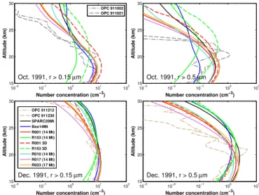
Figure 4.Cumulative particle number concentrations of OPC mea-surements (Deshler et al., 2003; Deshler, 2008), and model simula-tions in October 1991 (upper panels) and December 1991 (lower
panels) for particle size channels r >0.15 µm (left panels) and
r >0.5 µm (right panels).
volcanic aerosol. An increase in the distance of the volcanic plume above the tropopause will increase the lifetime of the volcanic aerosol due to a longer residence time for sediment-ing particles and a slower pathway of the aerosol within the Brewer-Dobson circulation. On the contrary, a larger initial mass loading may offset a higher injection altitude because of faster sedimentation caused by larger particles.
The results of “R001 3-D” using the coupled aerosol– chemistry–climate model SOCOL-AER is consistent (mostly within 10 %) with the AER 2-D simulation R001. In contrast, the consistency between R153 and “R153 3-D” is less satis-factory. The maximum aerosol burden simulated by “R153 3-D” is within 10 % of R153, but the e-folding time of the aerosol burden in the 3-D simulation (“R153 3-D”) is sig-nificantly faster (13 vs. 15 months) than in the 2-D simula-tion (R153). This indicates that in addisimula-tion to the initial mass loading and microphysics, model dynamics is essential to the decay of the volcanic aerosols. This difference between R153 (AER) and “R153 3-D” (SOCOL-AER) is possibly due to an insufficient rate of exchange of air between the troposphere and stratosphere in the AER 2-D model (Weisenstein et al., 1997) and/or a faster Brewer-Dobson circulation with respect to observations in the SOCOL (see the “tape recorder” in Fig. 8 of Stenke et al., 2013).
3.5 Matching particle size distributions
10−5 10−4 10−3 10−2 10−1 15
20 25 30
Altitude [km]
50−40°S
10−5 10−4 10−3 10−2 10−1
15 20 25 30
30−20°S
10−5 10−4 10−3 10−2 10−1
15 20 25 30
5°S−5°N
10−5 10−4 10−3 10−2 10−1
15 20 25 30
20−30°N
10−5 10−4 10−3 10−2 10−1
15 20 25 30
40−50°N
SAGE II v7 SPARC20Mt Box14Mt R001 R153 R001 3−D
R153 3−D
R010
R017
R033
10−5 10−4 10−3 10−2 10−1 15
20 25 30
Extinction [km−1]
Altitude [km]
10−5 10−4 10−3 10−2 10−1 15
20 25 30
Extinction [km−1]
10−5 10−4 10−3 10−2 10−1 15
20 25 30
Extinction [km−1]
10−5 10−4 10−3 10−2 10−1 15
20 25 30
Extinction [km−1]
10−5 10−4 10−3 10−2 10−1 15
20 25 30
Extinction [km−1]
Jan 1992
Jul 1992
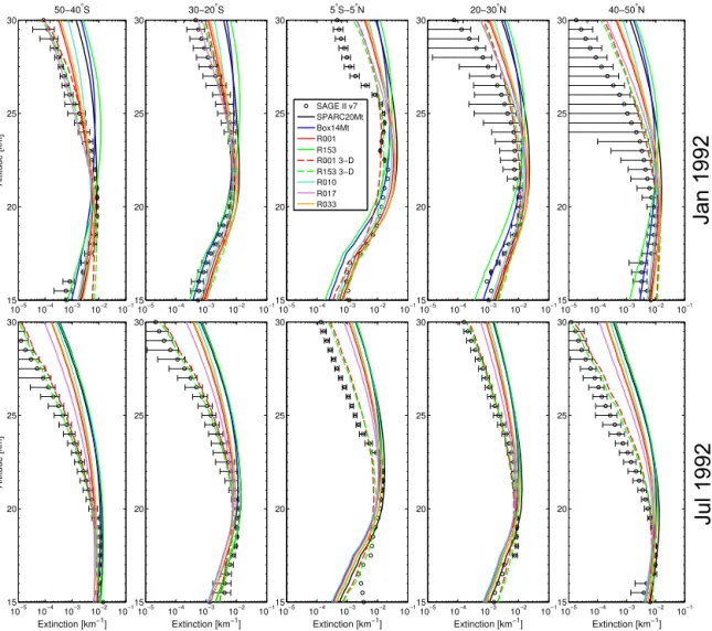
Figure 5.Aerosol 1020 nm extinction comparisons of SAGE II (version 7.0) and model simulations in five latitude bands (from left to right)
50–40◦S, 30–20◦S, 5◦S–5◦N, 20–30◦N and 40–50◦N for January (upper panel) and July 1992 (lower panel). Solid curves: AER 2-D
model results. Dashed curves: 3-D SOCOL-AER model results. Symbols with horizontal bars: SAGE II extinction measurements with bars indicating natural variability (namely observed zonal differences). Symbols without horizontal bars: data from individual ground-based lidar
stations used within SAGE-4λunder conditions when the atmosphere was so opaque that SAGE II could not measure it; so-called gap-filled
data with large uncertainty (SPARC, 2006; Luo, 2015).
0.5 µm). Below 23 km, R001 reasonably matches the ob-servations for r >0.15 µm, but less satisfactorily for r >
0.5 µm. The number density from R010 is slightly higher than R001 above∼24 km, which is consistent with the com-parison between initial vertical profiles of R001 and R010 (see Fig. 1). R017 agrees best with the observed number density, particularly above 24 km, because R017 emits very little SO2above 22 km. R033 predicts slightly higher
num-ber concentrations than R001 due to its larger initial mass loading (17 Mt SO2), but shows in general similar results
to R001. In contrast, the calculations from R153, Box14Mt and SPARC20Mt differ significantly from R001. Above 23 km, these three scenarios further overestimate the obser-vations than R001 because their initial injection profiles re-lease much more SO2 above 23 km compared to R001.
Be-low 23 km, R153 substantially underestimates the observa-tions in October 1991 as its injected mass locates mainly between 23–27 km, while Box14Mt shows better agree-ment with the observations (r >0.5 µm) below 18 km than R001, but largely underestimates the maximum near 21 km. SPARC20Mt is similar to R001 below 20 km since its initial mass loading (20 Mt SO2) compensates for the deficiency of
Latitude
AOT SAGE II
6 12 18 24 30 36 −60
−45 −30 −15 0 15 30 45 60
AOT R010 2D
6 12 18 24 30 36
−60 −45 −30 −15 0 15 30 45 60
Latitude
AOT R001 2D
6 12 18 24 30 36
−60 −45 −30 −15 0 15 30 45 60
AOT R153 2D
6 12 18 24 30 36
−60 −45 −30 −15 0 15 30 45 60
Latitude
AOT R017 2D
6 12 18 24 30 36
−60 −45 −30 −15 0 15 30 45 60
AOT SPARC20Mt 2D
6 12 18 24 30 36
−60 −45 −30 −15 0 15 30 45 60
Months since Jan 1991
Latitude
AOT R001 3D
6 12 18 24 30 36
−60 −45 −30 −15 0 15 30 45 60
1992 1993
Months since Jan 1991
AOT R153 3D
6 12 18 24 30 36
−60 −45 −30 −15 0 15 30 45 60
1992 1993
0.02 0.04 0.06 0.08 0.1 0.12 0.14 0.16 0.18
Figure 6. Aerosol optical thickness (AOT, 15–30 km) comparison between SAGE-4λ and model simulations. Marked regions in AOT SAGE II include gap-filled data. Triangle: time-latitude location of the Pinatubo eruption.
3.6 Matching extinctions
We compare the modeled 1020 nm extinctions with the gap-filled SAGE II version 7.0 (Fig. 5). SAGE II data points with horizontal bars are actual SAGE II measurements and de-note natural variabilities, while data points without bars are gap-filled from lidar ground stations, which have a higher uncertainty (SPARC, 2006). Figure 5 shows comparisons in January (upper panel) and July (lower panel) 1992 for five
latitude bands from left to right: 50–40◦S, 30–20◦S, 5◦S– 5◦N, 20–30◦N and 40–50◦N.
24 km. R033 is generally 10–20 % larger than R001 due to its higher initial mass loading, although it has the same verti-cal profile as R001. SPARC20Mt has even larger values than R033 due to a 20 Mt of SO2 mass loading. Box14Mt and
R153 largely overestimate the observed extinctions above 24 km. The 3-D simulation “R001 3-D” is superior to all the 2-D simulations, while “R153 3-D” performs worse than the 2-D simulations R001 and R033. Likewise, in June 1992, R001, R010 and R017 also do a better job than other 2-D simulations. The two 3-2-D simulations “R001 3-2-D” and “R153 3-D” are now both superior to all 2-D model results, although the differences between them start to shrink as the their aerosol burdens are now within 10 % from each other. Here the 3-D model shows a better extinction vertical pro-file likely because the 3-D model uses an improved numeri-cal scheme based on Walcek (2000) for sedimentation, while the 2-D model uses an upwind scheme, which would cause artificial upward transport of particles to high altitudes (Ben-duhn and Lawrence, 2013; Sheng et al., 2015). Evaporation of aerosol becomes important only above∼32 km, therefore should play a minor role in explaining the discrepancy be-tween the 2-D AER and 3-D SOCOL-AER. Overall, the re-sults from SPARC20Mt, Box14Mt, R033 and R153 display a common deficiency, as they tend to overestimate aerosol ex-tinctions in high altitudes above 24 km. Excessive mass load-ing (as in SPARC20Mt or R033) is one of the reasons. How-ever, the shape of the initial mass vertical profiles appears to be at least as important as the initial mass loading. Box14Mt has 30 % less total mass loading than SPARC20Mt, but it shows even higher extinctions in high altitudes because it has 40 % of its mass injected above 24 km, while SPARC20Mt has only about 20 % of its mass there.
Figure 6 compares the modeled aerosol optical thick-ness (AOT) with the SAGE II measurements. The south-ward transport of the volcanic clouds observed by SAGE II is reasonably reproduced by the models. The best scenar-ios here are R001 and R010, whose SO2 injection profiles
peak between 18–21 km and disperse the volcanic plume broadly (σ=4 km). In contrast, R017 with a narrow disper-sion (σ =2 km) constricts the initial SO2between 18–22 km,
which leads to a faster decay of AOT than R001 and R010. R153 and SPARC20Mt distribute too many aerosols to high latitudes due to injecting SO2excessively above 24 km. The
impact of the initial SO2vertical profile on the hemispheric
dispersion of the volcanic clouds is more pronounced in the 3-D simulations as shown in the two bottom panels. These results show that spatiotemporal distribution of the volcanic aerosols is affected by initial injection profile of SO2 and
the optimal parameters found in Table 1 would lead to better model results when compared to SAGE II observations.
4 Conclusions
We have conducted over 300 Pinatubo-like simulations by perturbing four parameters which determine the magnitude and vertical distribution of injected SO2. Our simulations
show that the initial SO2 magnitude and distribution play
a significant role in the evolution of stratospheric aerosol properties following the Pinatubo eruption, including rates of poleward transport of volcanic clouds. Our ensemble study suggests that Pinatubo injected less than 17 Mt of SO2into
the stratosphere, and that good agreement can be reached with a 14 Mt injection. The vertical profile of the injected SO2 is likely skewed towards the lower stratosphere, with
80 % of the SO2mass injected below 24 km and the
distribu-tion peak likely between 18 and 21 km. We have found a set of initial injection parameters such that the resulting model simulations fairly reproduce the evolution of stratospheric aerosol properties when compared to HIRS and SAGE II based data. This reduces the uncertainties in modeling the initial sulfur mass loading of Pinatubo.
Acknowledgements. This work was stimulated by the “Assessment of Stratospheric Aerosol Properties (ASAP)”, a previous activity of SPARC (Stratosphere-troposphere Processes and their Role in Climate). We thank Jason English and Anthony Baran for helpful discussion on HIRS measurements. We thank Laura Revell and Andrew Gettelman for useful suggestions on our work. We are particularly grateful to Mian Chin for valuable comments which helped to improve the manuscript. Thanks also to the unknown reviewers for their valuable comments. This work was supported by the Swiss National Science Foundation under the grant 200021-130478(IASSA).
Edited by: H. Tost
References
Aquila, V., Oman, L. D., Stolarski, R. S., Colarco, P. R., and New-man, P. A.: Dispersion of the volcanic sulfate cloud from a Mount Pinatubo–like eruption, J. Geophys. Res.-Atmos., 117, D06216, doi:10.1029/2011JD016968, 2012.
Arfeuille, F., Luo, B. P., Heckendorn, P., Weisenstein, D., Sheng, J. X., Rozanov, E., Schraner, M., Brönnimann, S., Thomason, L. W., and Peter, T.: Modeling the stratospheric warming follow-ing the Mt. Pinatubo eruption: uncertainties in aerosol extinc-tions, Atmos. Chem. Phys., 13, 11221–11234, doi:10.5194/acp-13-11221-2013, 2013.
Azzalini, A.: The Skew-normal Distribution and Related Multivari-ate Families, Scand. J. Stat., 32, 159–188, doi:10.1111/j.1467-9469.2005.00426.x, 2005.
Baran, A. J. and Foot, J. S.: New application of the operational sounder HIRS in determining a climatology of sulphuric acid aerosol from the Pinatubo eruption, J. Geophys. Res.-Atmos., 99, 25673–25679, doi:10.1029/94JD02044, 1994.
radia-tion management, J. Geophys. Res.-Atmos., 118, 7905–7921, doi:10.1002/jgrd.50622, 2013.
Bluth, G. J. S., Doiron, S. D., Schnetzler, C. C., Krueger, A. J., and
Walter, L. S.: Global tracking of the SO2clouds from the June,
1991 Mount Pinatubo eruptions, Geophys. Res. Lett., 19, 151– 154, doi:10.1029/91GL02792, 1992.
Crutzen, P. J.: Albedo Enhancement by Stratospheric Sulfur Injec-tions: A Contribution to Resolve a Policy Dilemma?, Climatic Change, 77, 211–220, doi:10.1007/s10584-006-9101-y, 2006. Deshler, T.: A review of global stratospheric aerosol:
Measure-ments, importance, life cycle, and local stratospheric aerosol, Atmos. Res., 90, 223–232, doi:10.1016/j.atmosres.2008.03.016, 2008.
Deshler, T., Hervig, M. E., Hofmann, D. J., Rosen, J. M., and Liley, J. B.: Thirty years of in situ stratospheric aerosol size
distri-bution measurements from Laramie, Wyoming (41◦N), using
balloon-borne instruments, J. Geophys. Res.-Atmos., 108, 4167, doi:10.1029/2002JD002514, 2003.
Dhomse, S. S., Emmerson, K. M., Mann, G. W., Bellouin, N., Carslaw, K. S., Chipperfield, M. P., Hommel, R., Abraham, N. L., Telford, P., Braesicke, P., Dalvi, M., Johnson, C. E., O’Connor, F., Morgenstern, O., Pyle, J. A., Deshler, T., Zawodny, J. M., and Thomason, L. W.: Aerosol microphysics simulations of the Mt. Pinatubo eruption with the UM-UKCA composition-climate model, Atmos. Chem. Phys., 14, 11221–11246, doi:10.5194/acp-14-11221-2014, 2014.
Dutton, E. G. and Christy, J. R.: Solar radiative forcing at selected locations and evidence for global lower tropospheric cooling fol-lowing the eruptions of El Chichón and Pinatubo, Geophys. Res. Lett., 19, 2313–2316, doi:10.1029/92GL02495, 1992.
English, J. M., Toon, O. B., and Mills, M. J.: Microphysical simula-tions of large volcanic erupsimula-tions: Pinatubo and Toba, J. Geophys. Res.-Atmos., 118, 1880–1895, doi:10.1002/jgrd.50196, 2013. Fero, J., Carey, S. N., and Merrill, J. T.: Simulating the dispersal of
tephra from the 1991 Pinatubo eruption: Implications for the for-mation of widespread ash layers, J. Volcanol. Geoth. Res., 186, 120–131, doi:10.1016/j.jvolgeores.2009.03.011, 2009.
Fleming, E. L., Jackman, C. H., Stolarski, R. S., and Con-sidine, D. B.: Simulation of stratospheric tracers using an improved empirically based two-dimensional model transport formulation, J. Geophys. Res.-Atmos., 104, 23911–23934, doi:10.1029/1999JD900332, 1999.
Guo, S., Bluth, G. J. S., Rose, W. I., Watson, I. M., and Prata, A. J.: Re-evaluation of SO2 release of the 15 June 1991 Pinatubo erup-tion using ultraviolet and infrared satellite sensors, Geochem., Geophys., Geosys., 5, Q04001, doi:10.1029/2003GC000654, 2004.
Heckendorn, P., Weisenstein, D., Fueglistaler, S., Luo, B. P., Rozanov, E., Schraner, M., Thomason, L. W., and Peter, T.: The impact of geoengineering aerosols on stratospheric temperature and ozone, Environ. Res. Lett., 4, 045108, doi:10.1088/1748-9326/4/4/045108, 2009.
Herzog, M. and Graf, H.-F.: Applying the three-dimensional model ATHAM to volcanic plumes: Dynamic of large co-ignimbrite eruptions and associated injection heights for volcanic gases, Geophys. Res. Lett., 37, L19807, doi:10.1029/2010GL044986, 2010.
Krueger, A. J., Walter, L. S., Bhartia, P. K., Schnetzler, C. C., Krotkov, N. A., Sprod, I., and Bluth, G. J. S.: Volcanic sulfur
dioxide measurements from the total ozone mapping spectrom-eter instruments, J. Geophys. Res.-Atmos., 100, 14057–14076, doi:10.1029/95JD01222, 1995.
Luo, B. P.: CCMI Aerosol Data – Release Version 2, ftp://iacftp. ethz.ch/pub_read/luo/ccmi/, last access: 3 October 2015. McCormick, M. P., Thomason, L. W., and Trepte, C. R.:
Atmo-spheric effects of the Mt Pinatubo eruption, Nature, 373, 399– 404, doi:10.1038/373399a0, 1995.
Niemeier, U., Timmreck, C., Graf, H.-F., Kinne, S., Rast, S., and Self, S.: Initial fate of fine ash and sulfur from large volcanic eruptions, Atmos. Chem. Phys., 9, 9043–9057, doi:10.5194/acp-9-9043-2009, 2009.
Notholt, J., Luo, B. P., Fueglistaler, S., Weisenstein, D., Rex, M., Lawrence, M. G., Bingemer, H., Wohltmann, I., Corti, T., Warneke, T., von Kuhlmann, R., and Peter, T.: Influ-ence of tropospheric SO2 emissions on particle formation and the stratospheric humidity, Geophys. Res. Lett., 32, L07810, doi:10.1029/2004GL022159, 2005.
Prinn, R. G., Huang, J., Weiss, R. F., Cunnold, D. M., Fraser, P. J., Simmonds, P. G., McCulloch, A., Harth, C., Reimann, S., Salameh, P., O’Doherty, S., Wang, R. H. J., Porter, L. W., Miller, B. R., and Krummel, P. B.: Evidence for variability of atmo-spheric hydroxyl radicals over the past quarter century, Geophys. Res. Lett., 32, L07809, doi:10.1029/2004GL022228, 2005. Read, W. G., Froidevaux, L., and Waters, J. W.: Microwave
limb sounder measurement of stratospheric SO2 from the Mt. Pinatubo Volcano, Geophysical Research Letters, 20, 1299– 1302, doi:10.1029/93GL00831, 1993.
Robock, A., MacMartin, D. G., Duren, R., and Christensen, M. W.: Studying geoengineering with natural and anthropogenic analogs, Climatic Change, 121, 445–458, doi:10.1007/s10584-013-0777-5, 2013.
Russell, P. B., Livingston, J. M., Pueschel, R. F., Bauman, J. J., Pol-lack, J. B., Brooks, S. L., Hamill, P., Thomason, L. W., Stowe, L. L., Deshler, T., Dutton, E. G., and Bergstrom, R. W.: Global to microscale evolution of the Pinatubo volcanic aerosol de-rived from diverse measurements and analyses, J. Geophys. Res.-Atmos., 101, 18745–18763, doi:10.1029/96JD01162, 1996. Sander, S., Abbatt, J., Barker, J., Burkholder, J., Friedl, R., Golden,
D., Huie, R., Kolb, C., Kurylo, M., Moortgat, G., Orkin, V., and Wine, P.: Chemical Kinetics and Photochemical Data for Use in Atmospheric Studies, Evaluation No. 17, JPL Publication 10-6, Jet Propulsion Laboratory, Pasadena, USA, 2011.
Sheng, J.-X., Weisenstein, D. K., Luo, B.-P., Rozanov, E., Stenke, A., Anet, J., Bingemer, H., and Peter, T.: Global atmospheric sulfur budget under volcanically quiescent conditions: Aerosol-chemistry-climate model predictions and validation, J. Geophys. Res. Atmos., 120, 256–276, doi:10.1002/2014JD021985, 2015. SPARC: SPARC Report No. 4, Assessment of Stratospheric
Aerosol Properties (ASAP), SPARC Report No. 4, edited by: Thomason, L. and Peter, Th., WMO, WCRP-124 WMO/TD No. 1295, 2006.
Stowe, L. L., Carey, R. M., and Pellegrino, P. P.: Monitoring the Mt. Pinatubo aerosol layer with NOAA/11 AVHRR data, Geo-phys. Res. Lett., 19, 159–162, doi:10.1029/91GL02958, 1992. Tabazadeh, A., Toon, O. B., Clegg, S. L., and Hamill, P.: A
new parameterization of H2SO4/H2O aerosol composition:
At-mospheric implications, Geophys. Res. Lett., 24, 1931–1934, doi:10.1029/97GL01879, 1997.
Thomason, L. W., Poole, L. R., and Deshler, T.: A global cli-matology of stratospheric aerosol surface area density deduced from Stratospheric Aerosol and Gas Experiment II measure-ments: 1984–1994, J. Geophys. Res.-Atmos., 102, 8967–8976, doi:10.1029/96JD02962, 1997.
Thomason, L. W., Burton, S. P., Luo, B.-P., and Peter, T.: SAGE II measurements of stratospheric aerosol properties at non-volcanic levels, Atmos. Chem. Phys., 8, 983–995, doi:10.5194/acp-8-983-2008, 2008.
Timmreck, C., Graf, H.-F., and Feichter, J.: Simulation of Mt. Pinatubo Volcanic Aerosol with the Hamburg Climate Model ECHAM4, Theoretical and Applied Climatology, 62, 85–108, doi:10.1007/s007040050076, 1999.
Toohey, M., Krüger, K., Niemeier, U., and Timmreck, C.: The influ-ence of eruption season on the global aerosol evolution and radia-tive impact of tropical volcanic eruptions, Atmos. Chem. Phys., 11, 12351–12367, doi:10.5194/acp-11-12351-2011, 2011. Walcek, C. J.: Minor flux adjustment near mixing ratio extremes
for simplified yet highly accurate monotonic calculation of tracer advection, J. Geophys. Res.-Atmos., 105, 9335–9348, doi:10.1029/1999JD901142, 2000.
Weisenstein, D. K., Yue, G. K., Ko, M. K. W., Sze, N.-D., Ro-driguez, J. M., and Scott, C. J.: A two-dimensional model of sul-fur species and aerosols, J. Geophys. Res., 102, 13019–13035, doi:10.1029/97JD00901, 1997.