The aerosol-climate model ECHAM5-HAM

(1)

ACPD

4, 5551–5623, 2004

The aerosol-climate model ECHAM5-HAM

P. Stier et al.

Title Page

Abstract Introduction

Conclusions References

Tables Figures

◭ ◮

Back Close

Full Screen / Esc

Print Version

Interactive Discussion

©EGU 2004

Atmos. Chem. Phys. Discuss., 4, 5551–5623, 2004 www.atmos-chem-phys.org/acpd/4/5551/

SRef-ID: 1680-7375/acpd/2004-4-5551 © European Geosciences Union 2004

Atmospheric Chemistry and Physics Discussions

The aerosol-climate model ECHAM5-HAM

P. Stier1, J. Feichter1, S. Kinne1, S. Kloster1, E. Vignati2, J. Wilson2,

L. Ganzeveld3, I. Tegen4, M. Werner4, Y. Balkanski5, M. Schulz5, and O. Boucher6

1

Max Planck Institute for Meteorology, Hamburg, Germany

2

Institute for the Environment and Sustainability, European Commission Joint Research Centre, Ispra, Italy

3

Max Planck Institute for Chemistry, Mainz, Germany

4

Max Planck Institute for Biogeochemistry, Jena, Germany

5

Laboratoire des Sciences du Climat et de l’Environnement, Gif-sur-Yvette, France

6

CNRS, USTL, Villeneuve d’Ascq, France

Received: 2 September 2004 – Accepted: 10 September 2004 – Published: 22 September 2004

(2)

ACPD

4, 5551–5623, 2004

P. Stier et al.

Title Page

Tables Figures

◭ ◮

Back Close

Full Screen / Esc

Print Version

©EGU 2004

Abstract

The aerosol-climate modelling system ECHAM5-HAM is introduced. It is based on a flexible microphysical approach and, as the number of externally imposed parameters is minimised, allows the application in a wide range of climate regimes. ECHAM5-HAM predicts the evolution of an ensemble of microphysically interacting

internally-5

and externally-mixed aerosol populations as well as their size-distribution and compo-sition. The size-distribution is represented by a superposition of log-normal modes. In the current setup, the major global aerosol compounds sulfate (SU), black carbon (BC), particulate organic matter (POM), sea salt (SS), and mineral dust (DU) are in-cluded. The simulated global annual mean aerosol burdens (lifetimes) for the year

10

2000 are for SO4: 0.80 Tg(S) (3.9 days), for BC: 0.11 Tg (5.4 days), for POM: 0.99 Tg (5.4 days), for SS: 10.5 Tg (0.8 days), and for DU: 8.28 Tg (4.6 days). An extensive evaluation with in-situ and remote sensing measurements underscores that the model results are generally in good agreement with observations of the global aerosol system. The simulated global annual mean aerosol optical depth (AOD) is with 0.14 in excellent

15

agreement with an estimate derived from AERONET measurements (0.14) and a com-posite derived from MODIS-MISR satellite retrievals (0.16). Regionally, the deviations are not negligible. However, the main patterns of AOD attributable to anthropogenic activity are reproduced.

1. Introduction

20

Atmospheric aerosols play an important role in the global climate system. Aerosol particles influence the global radiation budget directly, by scattering and absorption (Angstr ¨om˚ , 1962; McCormic and Ludwig, 1967), as well as indirectly, by the modi-fication of cloud properties (Twomey, 1974; Grassl, 1975; Twomey, 1977; Albrecht,

1989;Hansen et al.,1997;Lohmann,2002), with feedbacks to the hydrological cycle

25

(3)

reac-ACPD

4, 5551–5623, 2004

P. Stier et al.

Title Page

Tables Figures

◭ ◮

Back Close

Full Screen / Esc

Print Version

©EGU 2004

tions on the aerosol surface and in liquid aerosol particles interact with the chemistry of the atmosphere (Ravishankara,1997;Andreae and Crutzen,1997;Crutzen,1996;

Dentener and Crutzen,1993). Pollutants, such as DDT, condense on aerosol particles so that their transport and deposition are largely determined by the aerosol pathways (van Pul et al.,1998;Unsworth et al., 1999). Moreover, the deposition of aerosol in

5

the ocean plays an important role in the biogeochemical cycle of the oceans (Vink and

Measures,2001;Johnson et al.,1997).

Nevertheless, the quantitative comprehension of the role of aerosols is still insu_ffi -cient (e.g.Penner et al.,2001;Ramanathan et al.,2001;Heintzenberg et al.,2003).

To increase the understanding of this complex system, the ECHAM5 General

Circu-10

lation Model (GCM) (Roeckner et al.,2003) has been extended by a complex aerosol model allowing long-term transient climate simulations. A major objective is to quantify the aerosol radiative effects and their impacts on the global climate system for present day and future conditions.

Most previous studies of the global aerosol system (e.g.Langner and Rhode,1991;

15

Feichter et al.,1996;Roelofs et al.,1998;Lohmann et al.,1999a;Rasch et al.,2000;

Chin et al., 2002) have simulated the global distribution of the mass of one or more of the major aerosol components: sulfate (SU), elemental carbon, henceforth denoted as black carbon (BC), particulate organic matter (POM), sea salt (SS), and mineral dust (DU). In these studies aerosol is either represented by an external mixture (e.g.

20

Lohmann et al.,1999a;Tegen et al.,1997) or by an internal mixture with a fixed ratio of the individual components (e.g.Haywood et al.,1997b). An internal mixture refers to the assumption that all particles contain a uniform mixture of the individual compo-nents whilst an external mixture describes a mixture of particles each of which is made of solely one compound. However, observations show (e.g.Murphy et al.,1998;Bates 25

(4)

An-ACPD

4, 5551–5623, 2004

P. Stier et al.

Title Page

Tables Figures

◭ ◮

Back Close

Full Screen / Esc

Print Version

©EGU 2004

other drawback of the bulk modelling approach is that in order to calculate direct and indirect radiative e_ffects, as well as the sinks of the aerosol mass itself, implicit assump-tions about the aerosol size distribution have to be imposed. Many feedback cycles are highly sensitive to aerosol number and therefore to the size-distribution. In short, a comprehensive analysis of aerosol-climate interactions, including feedback processes,

5

requires knowledge of the size-distribution, the composition, and the mixing state and therefore size-segregated, microphysical, multicomponent aerosol modules suitable for long-term integrations.

Tegen and Lacis (1997) simulated the size-distribution and radiative properties of mineral dust in a GCM with size-dependent sources and sinks without interaction

10

among the size classes. Adams and Seinfeld (2002) predicted the size-distribution of sulfate aerosol with an interactive approach. A number of studies, (e.g.Tegen et al.,

1997; Jacobson, 2001; Takemura et al., 2000), incorporated partly size-segregated aerosol modules with several components into global aerosol models, neglecting the microphysical interaction among the components. Only recently, size-segregated,

in-15

teractive multicomponent aerosol modules are embedded into global models allowing to simulate the mixing state explicitly.Wilson et al.(2001) represent the size-distribution in a multicomponent aerosol model by a superposition of eight partly interacting log-normal modes. Ghan et al.(2001a,b) use an interactive modal size-segregated multi-component module to estimate the direct and indirect radiative aerosol forcing. Gong 20

et al. (2003) describe the development of a size-segregated aerosol module and apply it to the simulation of the global sea-salt distribution (Gong et al.,2002). They have the option to treat fresh emissions as external mixture with a fixed aging time, assuming that the aging only occurs in the emission grid box.

In the development of the ECHAM5-HAM aerosol model the attempt was made to

25

(5)

ACPD

4, 5551–5623, 2004

P. Stier et al.

Title Page

Tables Figures

◭ ◮

Back Close

Full Screen / Esc

Print Version

©EGU 2004

of size and composition. This setup allows the prediction of the aerosol radiative effects directly from the prognostic variables and provides the necessary parameters for the aerosol-cloud coupling. Computational e_fficiency of this aerosol model permits the application in long-term climate studies.

Section2describes the setup of the ECHAM5-HAM model. Results from a

simula-5

tion for the year 2000 and their evaluation are presented in Sect.3. Section4concludes the discussion and presents an outlook to future developments.

2. Model description

2.1. The ECHAM5 general circulation model

The atmospheric general circulation model ECHAM5 is the fifth-generation climate

10

model developed at the Max Planck Institute for Meteorology, evolving from the model of the European Centre for Medium-Range Weather Forecasts (ECMWF). ECHAM5 solves prognostic equations for vorticity, divergence, surface pressure and tempera-ture expressed in terms of spherical harmonics with a triangular truncation. Water vapour, cloud liquid water, cloud ice and trace components are transported with a flux

15

form semi-Lagrangian transport scheme (Lin and Rood, 1996) on a Gaussian grid.

ECHAM5 contains a new microphysical cloud scheme (Lohmann and Roeckner,1996)

with prognostic equations for cloud liquid water and ice. Cloud cover is predicted with a prognostic-statistical scheme solving equations for the distribution moments of total water (Tompkins,2002). Convective clouds and convective transport are based on the

20

mass-flux scheme ofTiedtke (1989) with modifications byNordeng(1994). The solar radiation scheme (Fouquart and Bonnel,1980) has 4 spectral bands, 1 for the visible and ultra-violet, and 3 for the near-infrared. The long-wave radiation scheme (Mlawer

et al.,1997;Morcrette et al., 1998) has 16 spectral bands. ECHAM5 has the capa-bility to perform nudged simulations, i.e. to relaxate the prognostic variables towards

25

(6)

ACPD

4, 5551–5623, 2004

P. Stier et al.

Title Page

Tables Figures

◭ ◮

Back Close

Full Screen / Esc

Print Version

©EGU 2004

weather forecast models.

2.2. The modal concept

A fine discretisation of the wide aerosol spectrum is with current computational re-sources not efficient for the long term global prediction of interactive multicomponent aerosol distributions and their mixing state. Thus, the aerosol spectrum in HAM is

5

represented by the superposition of seven log-normal distributions:

n(lnr)=

7

X

i=1

Ni

√ 2πlnσi

exp ₋(lnr−ln ¯ri)

2

2 ln2σ_i !

. (1)

Each modei of the aerosol number distribution can be described by the three mo-ments aerosol numberN_i, the number median radius ¯r_i, and the standard deviation

σ_i. In HAM it is assumed that the standard deviation is constant and set to σ =1.59

10

for the nucleation, Aitken, and accumulation modes and to σ = 2.00 for the coarse modes. Thus, it is possible to calculate the median radius of each mode from the cor-responding aerosol number and aerosol mass, which are transported as tracers. The modes of the aerosol model are composed either of compounds with no or low solu-bility, henceforth denoted as insoluble mode, or by an internal mixture of insoluble and

15

soluble compounds, henceforth denoted as soluble mode.

The relative composition of each internally mixed mode can be modified by aerosol dynamics, e.g. coagulation, by thermodynamical processes, e.g. condensation of sul-fate on pre-existing particles, and by cloud processing. In this study we describe an implementation of the aerosol model with following components: sulfate, black carbon,

20

organic matter, sea salt, and mineral dust. However, ECHAM5-HAM is flexible to be

extended to more compounds. Table 1 illustrates the modal setup and the

(7)

ACPD

4, 5551–5623, 2004

P. Stier et al.

Title Page

Tables Figures

◭ ◮

Back Close

Full Screen / Esc

Print Version

©EGU 2004

2.3. Emission module

With the exception of the sulfur compounds, all emissions are treated as primary emis-sions, i.e. the compounds are assumed emitted as particulate matter. This is a phys-ical assumption for most of the treated species. However, it is only a proxy for the particulate fraction of organic matter. Extending the parameter space of the aerosol

5

model to include aerosol numbers requires the knowledge of the size distribution of the emitted particles. Additionally, the application of emissions in a GCM implies the assumption of homogeneous mixing across the model grid box with a typical scale of more than 100 km. The emissions of dust, sea salt and oceanic dimethyl sulfide (DMS) are calculated online. Terrestrial biogenic DMS emissions are prescribed. For

10

all other compounds, emission strength, distribution, and height are based on the AE-ROCOM (http://nansen.ipsl.jussieu.fr/AEROCOM/) emission inventory for the aerosol model inter-comparison experiment B (Dentener, in preparation) representative for the

year 2000. The emission scenario is summarised in Table 2 and explained in more

detail in the following paragraphs.

15

2.3.1. Sulfur Emissions

We consider natural DMS emissions from the marine biosphere. The emission flux is calculated interactively from DMS seawater concentrations of Kettle and Andreae

(2000) utilising the ECHAM5 10 m wind speed to derive the air-sea exchange rate following Nightingale et al. (2000). Terrestrial biogenic emissions in form of DMS

20

are applied from Pham et al. (1995). Non-eruptive volcanic sulfur emissions are taken fromAndres and Kasgnoc(1998) supplemented by eruptive emissions with lo-cations following Halmer et al. (2002) and a total strength recommended by GEIA (http://www.geiacenter.org). Non-eruptive emissions are distributed between the vol-cano height and one third below, eruptive emissions are distributed 500 to 1500 m

25

(8)

ACPD

4, 5551–5623, 2004

P. Stier et al.

Title Page

Tables Figures

◭ ◮

Back Close

Full Screen / Esc

Print Version

©EGU 2004

(van der Werf et al., 2003). Emissions from industry, power-plants, and shipping are distributed between 100 and 300 m above surface. Vegetation fires inject emissions in heights well above the surface. We account for that by prescribing emission profiles derived from measured ecosystem specific injection heights (Lavou ´e, pers. comm.), ranging from 0 to 6 km. Except for DMS, we assume 97.5% of all sulfuric emission in

5

the form of SO₂ and 2.5% in the form of primary sulfate. 50% of ship-, industrial-, and power-plant emissions are attributed to the accumulation mode with a number median radius ¯r =0.075 µm andσ=1.59 and 50% to the coarse mode with ¯r =0.75 µm and

σ=2.00. Other primary sulfate emissions are attributed with 50% to the Aitken mode with ¯r =0.03 µm andσ=1.59 and with 50% to the accumulation mode with ¯r =0.075

10

andσ =1.59.

2.3.2. Carbonaceous Emissions

Fossil-fuel and bio-fuel emissions for black and organic matter are used from Bond

et al. (2004) assuming an emission size distribution with a number median radius of ¯r = 0.015 µm and σ = 1.59. For carbonaceous emissions from vegetation fires

15

(van der Werf et al.(2003) we assume ¯r =0.04 µm andσ=1.59 and injection heights as described in Sect.2.3.1. The biogenic monoterpene emissions ofGuenther et al.

(1995), are scaled by the factor 0.15 to estimate the production of Secondary Organic Aerosol (SOA) from biogenic sources. Black carbon emissions are assumed insoluble and 65% of the POM emissions are assumed soluble. The soluble fraction of POM is

20

assumed to condense on the soluble modes, the insoluble fraction is emitted in par-ticulate form in the insoluble Aitken mode. For the conversion of the carbon mass of POM into the total mass of POM, a factor of 1.4 is applied.

2.3.3. Sea Salt Emissions

Sea salt aerosol is produced by wind-induced formation of sea spray and its

subse-25

(9)

func-ACPD

4, 5551–5623, 2004

P. Stier et al.

Title Page

Tables Figures

◭ ◮

Back Close

Full Screen / Esc

Print Version

©EGU 2004

tions have been developed, parameterising the emission flux as a function of the 10 m wind speed. Guelle et al.(2001) show that the emission source function can best be represented by a combination of the approach ofMonahan et al.(1986) for the small particle range and ofSmith and Harrison(1998) for the coarse particle range. Follow-ing their approach we merge the source functions smoothly in the size range 2–4 µm

5

dry radius and fit the combined source function by two lognormal distributions. The mass median radii as a function of wind speed decrease with increasing wind speed of 1 to 40 m s−1from 0.284 to 0.271 µm and from 2.25 to 2.15 µm for the two modes, respectively (Schulz et al., in preparation).

2.3.4. Dust Emissions

10

For the emission of mineral dust, two optional schemes have been implemented into HAM: the scheme ofTegen et al. (2002) and the scheme of Balkanski et al.(2003). Both schemes are coupled online, i.e. they calculate the emission of mineral dust in dependence of the ECHAM5 wind speed and hydrological parameters. Freshly emit-ted dust is assumed insoluble.Tegen et al.(2002) derive preferential dust source areas

15

from an explicit simulation of paleological lakes. In addition, lower dust emissions can occur in other non-vegetated regions. The emission flux is then calculated from 192 internal dust size-classes and the explicit formulation of the saltation process following

Marticorena and Bergametti(1995).Balkanski et al.(2003) have associated threshold velocities derived byMarticorena and Bergametti(1995) to the mineralogical

composi-20

tion of the di_fferent soil types of the Food And Agriculture Organization Of The United Nations (http://www.fao.org) over the same region. This allowed to extend the domain to obtain a global dust source formulation (Claquin,1999). In addition, regional source strength were deduced for 12 arid regions by adjusting model optical depth to optical depth deduced from TOMS aerosol indices (Hsu et al.,1999).

25

For the implementation of the Tegen et al.(2002) scheme into ECHAM5-HAM, we

(10)

life-ACPD

4, 5551–5623, 2004

P. Stier et al.

Title Page

Tables Figures

◭ ◮

Back Close

Full Screen / Esc

Print Version

©EGU 2004

time and the negligible contribution of the super-coarse mode to the radiative effect, we neglect the super-coarse mode emissions and apply the emission into the insoluble accumulation and coarse modes with mass-median radii of 0.37 µm and 1.75 µm and standard deviations of 1.59 and 2.00, respectively. For the Balkanski et al. (2003) scheme we also neglect the super-coarse mode emissions and emit into the insoluble

5

coarse mode with a mass-median radius of 1.25 µm and a standard deviation of 2.00. A full description and comparison of the results of the two dust schemes is beyond the scope of this paper. Thus, unless otherwise quoted, we will focus henceforth on the results from theTegen et al.(2002) scheme.

2.4. Chemistry module

10

The chemistry module is based on the sulfur cycle model as described by Feichter

et al. (1996) treating the prognostic variables dimethyl sulfide (DMS), sulfur dioxide (SO₂) and sulfate (SO2₄−). Three dimensional monthly mean oxidant fields of OH, H₂O₂, NO₂, and O₃are prescribed from calculations of the comprehensive MOZART chemical transport model (Horowitz et al.,2003). In the gas phase, DMS and SO₂are oxidised

15

by hydroxyl (OH) and DMS reacts with nitrate radicals (NO₃). In the aqueous phase the oxidation of SO₂ by H₂O₂ and O₃ are considered. The aqueous phase concentration of SO₂is calculated according to Henry’s law, accounting for dissolution e_ffects.

Gas-phase produced sulfate is attributed to the gaseous phase and allowed to be condensated on pre-existing particles or nucleated by the aerosol microphysics

mod-20

(11)

ACPD

4, 5551–5623, 2004

P. Stier et al.

Title Page

Tables Figures

◭ ◮

Back Close

Full Screen / Esc

Print Version

©EGU 2004

2.5. Deposition module

2.5.1. Dry deposition

The net surface fluxes, calculated by subtracting the dry deposition fluxes from the re-spective emission fluxes, provide the lower boundary conditions for the implicit vertical diffusion scheme of ECHAM5. The dry deposition flux is calculated as the product of

5

the surface layer concentration and the dry deposition velocity:

Fd =Cρairvd, (2)

whereCis the tracer mass or number mixing ratio of the tracer,ρ_air is the air density, andvd is the dry deposition velocity. The dry deposition velocities are calculated based

on a serial resistance approach.

10

For gases,v_d is calculated from the aerodynamic, quasi-laminar boundary layer, and surface resistance according to the “big leaf” concept (Ganzeveld and Lelieveld,1995;

Ganzeveld et al.,1998) for the ECHAM5 fractional surface cover types (snow/ice, bare soil, vegetation, wet skin, water and sea ice) of each grid box. The surface resistances are generally prescribed except of some specific resistances, e.g. the SO₂ soil

resis-15

tance as a function of soil pH, relative humidity, surface temperature, and the canopy resistance. The latter is calculated from ECHAM5’s stomatal resistance and a monthly mean Leaf Area Index (LAI) inferred from a NDVI (Normalised Differential Vegetation Index) climatology (Gutman et al.,1995) and theOlson(1992) ecosystem database.

For aerosols we have implemented the dry deposition velocity model that has

pre-20

viously been applied to develop a sulfate aerosol dry deposition parameterisation (Ganzeveld et al., 1998). In contrast to using prescribed sulfate mass size distribu-tions, which were used to develop the sulfate aerosol dry deposition parameterisation, we use in this study the explicitly calculated modal number and mass parameters to calculate the aerosol dry deposition velocity as a function of particle radius, density,

tur-25

(12)

ACPD

4, 5551–5623, 2004

P. Stier et al.

Title Page

Tables Figures

◭ ◮

Back Close

Full Screen / Esc

Print Version

©EGU 2004

soil and snow/ice aerosol dry deposition velocities according Slinn (1976), over wa-ter according toSlinn and Slinn (1980), whereas the vegetation and wet skin aerosol dry deposition velocities are calculated according toSlinn(1982) andGallagher et al.

(2002). Over water, the effect of whitecaps in enhancing aerosol dry deposition ac-cording toHummelshøj et al.(1992) is taken into account.

5

2.5.2. Sedimentation

Sedimentation of the aerosol particles is calculated throughout the atmospheric col-umn. The calculation of the sedimentation velocity is based on the Stokes velocity

vs =

2 9

r2ρgC_c

µ (3)

with the Cunningham slip-flow correction factor Cc accounting for non-continuum ef-10

fects (e.g.Seinfeld and Pandis,1998):

C_c=1₊λ

r

1.257₊0.4 exp₋1.1r

λ

. (4)

Hereby is v_s the sedimentation velocity, r the number or mass median radius, ρ the particle density,g the gravitational acceleration, µthe gas viscosity, and λthe mean free path of air. To satisfy the Courant-Friedrich-Lewy stability criteria, the

sedimenta-15

tion velocity is limited tov_s < ∆z

∆t where∆z is the layer thickness and∆t is the model

timestep.

2.5.3. Wet deposition

The fraction of scavenged tracers is calculated from the in-cloud content utilising the precipitation formation rate of the ECHAM5 cloud scheme. For gases, the

partition-20

ing between the air and the cloud water is calculated based on Henry’s law (see e.g.

(13)

size-ACPD

4, 5551–5623, 2004

P. Stier et al.

Title Page

Tables Figures

◭ ◮

Back Close

Full Screen / Esc

Print Version

©EGU 2004

and composition-dependent scavenging parameterR. R is defined as the fraction of the tracer in the cloudy part of the grid box that is embedded in the cloud liquid/ice water. Values ofRfor stratiform clouds follow measurements of interstitial and in-cloud aerosol contents ofHenning et al.(2004), with slight modifications, and for ice clouds are based onFeichter et al. (2004). It should be noted that for the accumulation and

5

coarse modeRis lower for mixed phase clouds then for liquid clouds due to the growth of ice crystals at the expense of water droplets as a result of the Bergeron-Findeisen process (Henning et al.,2004). For convective clouds, few size-resolved measurement data is available. Thus, assuming higher supersaturations and therefore activation into lower size-ranges, we increaseR in convective clouds for the soluble modes, which

10

we assume to be potential cloud condensation nuclei. The prescribed values ofR are given in Table3.

For the scavenging by stratiform clouds, the local rate of change of traceri is calcu-lated as:

∆C_i

∆t =

R_iC_ifcl Cwat

Qliq fliq +

Qice fice

!

, (5)

15

whereCi,Cwat are mixing ratios of the tracer i and total cloud water, respectively. f cl

is the cloud fraction,fliqandfice are the liquid- and ice fraction of the cloud water. Qliq

andQiceare the respective sum of conversion rates of cloud liquid water and cloud ice to precipitation, via the processes auto-conversion, aggregation, and accretion.

Convective scavenging is coupled with the mass flux scheme of the convective tracer

20

transport. In addition to the local change of the tracer tendency, the convective tracer fluxes have to be adjusted by the wet deposition. In convective updrafts the tracer mix-ing ratios are associated with the liquid- and ice-phase proportionally to the presence of the respective phase:

C_iliq=Cifliq C_iice=Cifice. (6)

(14)

ACPD

4, 5551–5623, 2004

P. Stier et al.

Title Page

Tables Figures

◭ ◮

Back Close

Full Screen / Esc

Print Version

©EGU 2004

The change in tracer mixing ratio is calculated as

∆C_i = ∆Cliq_i + ∆C_iice=C_iliqR_iEliq+C_iiceR_iEice, (7)

whereRi is the scavenging parameter and Eliq and Eice are the fractions of updraft

liquid water and updraft ice water that are converted into precipitation during one timestep.

5

From the local_∆C_i for each layerkthe local grid-box mean deposition fluxF_id epand the grid-box mean tendency∆C_i/∆tare calculated:

F_id ep = ∆C_iFup ∆Ci

∆t =F

d ep i

g

∆p (8)

Hereby isFup _{the grid-box mean updraft mass flux. The local deposition flux is}

inte-grated from the model top to the respective layerk:

10

F_idep

int

=

k

X

top

F_idep. (9)

The mean updraft tracer fluxF_iup for tracer i is recalculated based on the updated updraft tracer mixing ratios:

F_iup=(Ci −∆Ci)Fup. (10)

A non-negligible fraction of precipitation re-evaporates before it reaches the ground.

15

Re-evaporation acts on the integrated tracer deposition fluxF_idep

int

proportionally to the evaporation of precipitation:

∆F_idep

int

=F_idep

int

(15)

ACPD

4, 5551–5623, 2004

P. Stier et al.

Title Page

Tables Figures

◭ ◮

Back Close

Full Screen / Esc

Print Version

©EGU 2004

∆Ci

∆t = ∆F

d ep i

i nt _g

∆p, (12)

where fevap is the evaporating fraction of precipitation, ∆p is the layer thickness in pressure units, andgis the gravitational acceleration.

For aerosols, below-cloud scavenging is calculated from the ECHAM5 water- and ice-precipitation fluxes with prescribed size-dependent collection efficiencies R_ir and

5

R_is from Seinfeld and Pandis (1998) for rain and snow, normalised by the respective precipitation rate

∆Ci

∆t =C

amb i f

precip _Rr iF

r

+R_isFs

, (13)

whereCamb_i is the mass mixing ratio of the ambient cloud free air,fprecipis the e_ffective grid-box fraction a_ffected by precipitation, and Fr and Fs are the fluxes of rain and

10

snow, respectively. fprecip is estimated in the stratiform scheme by the assumption of maximum overlap of the cloudy parts of the grid box and for the convective scheme from the estimated updraft area.

2.6. Relative humidity

Sub-grid scale variations in relative humidity can have a large impact on the water

15

uptake of aerosols and their radiative forcing (e.g.Haywood et al., 1997a). As cloud processing of aerosols and cloud radiative effects predominate in the cloudy part of the grid box, it is desirable to apply ambient conditions for the aerosol microphysics and thermodynamics in the cloud free part. The usage of the grid mean relative humidity

RH=q/qs leads to an overestimation ofRH in the cloud free part of a partly clouded

20

(16)

ACPD

4, 5551–5623, 2004

P. Stier et al.

Title Page

Tables Figures

◭ ◮

Back Close

Full Screen / Esc

Print Version

©EGU 2004

respectively. This assumption allows to calculate the relative humidity in the cloud-free part of the grid box:

RHamb= q

amb

qs , (14)

where the ambient specific humidityqambis calculated from

q=qsfcl+qamb(1₋fcl), (15)

5

wherefclis the cloud fraction.

Turbulent sub-grid scale fluctuations ofRH are not accounted for in this study.

2.7. The aerosol microphysics module M7

The microphysical core of the ECHAM5-HAM aerosol model is the aerosol module M7 (Vignati et al.,2004) evolving from an earlier version M3+that has already been used

10

and tested in global aerosol modelling studies with offline chemical transport models (Wilson et al., 2001). M7 treats the aerosol dynamics and thermodynamics in the framework of the modal structure that is described in the Sect.2.2. Only the major processes in M7 are described here as a thorough description and evaluation of M7 can be found in (Vignati et al.,2004).

15

2.7.1. Coagulation

The computation of the coagulation is computationally expensive. Therefore, the dom-inating processes have been identified during the development of M7 by theoretical considerations and case studies and only those are calculated explicitly. The calcu-lation of the coagucalcu-lation coefficients is based on a parameterisation of the Brownian

20

(17)

ACPD

4, 5551–5623, 2004

P. Stier et al.

Title Page

Tables Figures

◭ ◮

Back Close

Full Screen / Esc

Print Version

©EGU 2004

i and j is:

Ki j =

16πr˜D˜

4 ˜D ˜ νr˜ +

˜ r ˜ r+_∆˜

, (16)

where ˜D, ˜νand ˜∆ are the diffusion coefficient, the thermal velocity and the mean free path length for particles with a mean radius of ˜r =r¯i+r¯j

2 , respectively.

2.7.2. Condensation

5

Under sulfate-limited conditions, the condensation of sulfate on potentially pre-existing particles and the nucleation of new sulfate particles compete for the available gas phase sulfate. As the condensation of sulfate on pre-existing particles is energetically favoured due to the Kelvin e_ffect, the partitioning of sulfate between those processes is treated in M7 as follows:

10

In a first step, the total maximum amount of condensable sulfate on pre-existing particles is calculated. This process is limited by the availability of gas phase sulfate and the di_ffusion of the sulfate to the surface of the particles. The calculation follows the methodology ofFuchs(1959) matching the diffusion in the kinetic and continuous regimes. The distinction between condensation on insoluble and on mixed/insoluble

15

particles is realized by the assumption of di_fferent accommodation coe_fficients ofα =

0.3 for the insoluble andα =1.0 for the soluble particles.

In the second step, the remaining gas phase sulfate is available for the nucleation of new clusters.

2.7.3. Nucleation

20

(18)

ACPD

4, 5551–5623, 2004

P. Stier et al.

Title Page

Tables Figures

◭ ◮

Back Close

Full Screen / Esc

Print Version

©EGU 2004

gas-phase concentration of the after the condensation available sulfate (see2.7.2) the number of nucleated particles as well as the integral mass of the nucleated sulfate is parameterised following Vehkam ¨aki et al. (2002). Compared to the earlier tested and optionally available scheme byKulmala et al.(1998) this scheme has the advan-tage of an extended range of thermodynamical conditions (0.01% < RH < 100%,

5

230.15 K< T <305.15 K) and the usage of a more stringent application of nucleation theory. The predicted nucleation rate is then integrated analytically to calculate the number of nucleated particles over one timestep. The corresponding nucleated mass of sulfate is then derived based on the predicted nucleation cluster size starting at four molecules.

10

2.7.4. Thermodynamics

For particles containing sulfate, the calculation of the thermodynamical equilibrium with the water vapour phase is based on a generalised form of the Kelvin equation. For computational efficiency the parameterisation is realized in form of a look-up table. The calculation of the water content of particles that contain beside sulfate insoluble

15

components, such as dust or black carbon, is done analogous to pure sulfate particles but with the dry radii of the total compounds.

With increasing ambient relative humidity, when the humidity reaches the Deliques-cence Relative Humidity (DRH), particles containing sea salt grow spontaneously by water uptake from the surrounding air. With decreasing ambient humidity, the sea salt

20

aerosol releases the up-taken water not until a relative humidity well below theDRH, the so called Ephlorescence Relative Humidity (E RH). This hysteresis phenomenon is not taken into account in the current version of M7. In fact, as sea-salt aerosol is formed from the evaporation of larger droplets, it is assumed that particles do not re-lease their water down toE RH =45% (fromTang,1997). The aerosol water content

(19)

ACPD

4, 5551–5623, 2004

P. Stier et al.

Title Page

Tables Figures

◭ ◮

Back Close

Full Screen / Esc

Print Version

©EGU 2004

of particles containing sea salt in conditions ofRH > E RH is calculated as follows.

W =X

i

c_i mi

. (17)

Hereby are W the aerosol water content [g m−3], ci concentration of compound i

[mol m−3] and mi the binary molality of compound i [mol g−1]. It is assumed, based

on the ZSR-Relation (Zadanovskii,1948;Stokes and Robinson,1966), that the water

5

activity of mixtures of electrolytes is equal to the water activity of the binary electrolyte-water mixture. The calculation of the binary molalities is done as follows

mi =





7

X

j=0

Yj (RH)j





2

, (18)

whereRH is the relative humidity (water activity) andYj are empirical coefficients from Jacobson et al.(1996).

10

2.7.5. Integration of the aerosol dynamics equation

Analytical solutions are applied to integrate the aerosol dynamics equation for each mode, calculating the updated aerosol numbers and the transfer between the modes.

The aerosol dynamics equation for the soluble modes (1_≤i ≤ns) can be expressed as:

15

d N_i d t =−

1 2Ki iN

2

i (19)

−N_i





ns

X

j=i+1

K_{i j}N_j +

ns+ni

X

j=i+ns

K_{i j}N_j 

+δ_i₁c.

(20)

ACPD

4, 5551–5623, 2004

P. Stier et al.

Title Page

Tables Figures

◭ ◮

Back Close

Full Screen / Esc

Print Version

©EGU 2004

particle number,K_{i j} the coagulation coefficient for the coagulation of modei and mode

j, and c the nucleation rate. The inter-modal coagulation consists of a contribution of coagulation with larger soluble modes as well as a contribution of coagulation with particles of larger insoluble modes.

For the insoluble modes, the coagulation also with smaller soluble particles is a sink

5

as in this case the particles are transferred to the soluble/mixed mode. The coagulation with higher insoluble modes however, is considered inefficient for the insoluble modes. Therefore, the aerosol dynamics equation for the insoluble modes (ns+1_≤i ≤ns+ni) can be expressed as

d Ni

d t =−

1 2Ki iN

2 i −Ni





ns

X

j=1

K_{i j}N_j 

. (20)

10

The first term on the right hand side, representing the intra-modal coagulation, is negligible and thus omitted for the insoluble dust modes. The second term of the right hand side, accounting for the inter-modal coagulation with soluble modes, is treated operator split in a subsequent procedure (see Sect.2.7.6).

From the analytically integrated changes in the aerosol numbers, the corresponding

15

aerosol mass concentrations are then calculated mass conserving by summing up the number of particles transferred between the modes and multiplication with the respec-tive mean particle masses.

2.7.6. Transfer from the insoluble- to the mixed-modes

Particles in the insoluble modes are transformed to the corresponding soluble/mixed

20

mode by condensation of sulfate on their surface or by coagulation with particles of soluble modes. The total condensable sulfate on the respective mode (see2.7.2) and the sulfate added to this mode by coagulation are attributed to the number of particles that can be coated with a minimal layer of sulfate. We assume a mono-layer for this minimal layer thickness. Particle numbers and masses of the coated particles, as

(21)

ACPD

4, 5551–5623, 2004

P. Stier et al.

Title Page

Tables Figures

◭ ◮

Back Close

Full Screen / Esc

Print Version

©EGU 2004

well as the through condensation and coagulation available sulfate mass, are then transferred to the corresponding soluble mode.

2.7.7. Repartitioning between the modes

The previously described processes would cause a significant overlap between the modes. For example, nucleation mode particles typically grow by coagulation and

con-5

densation via the Aitken mode into the accumulation mode. Numerically, this leads to the fact that the mode median radius, but also the mode standard deviation, would increase steadily, associated with numerical diffusion. A mode merging algorithm (

Vig-nati et al.,2004) is applied to repartition the particles among the modes and to confine the number median radius of each mode to the range given in Table1.

10

2.8. Radiation module

The prognostic treatment of size-distribution, composition, and mixing state allows the explicit calculation of the aerosol optical properties in the framework of the Mie theory. However, the online calculation of the aerosol optical properties is computationally ex-pensive. Therefore, the required aerosol optical properties are pre-computed from Mie

15

theory for 24 solar spectral bands, followingToon and Ackerman(1981), and supplied in look-up tables with the three dimensions: Mie size-parameter (X =2πr/λ), and real-and imaginary part (n_r andn_i) of the refractive index. Herebyr is the number median

radius of the log-normal mode andλ is the wavelength. The geometric arrangement

of internally mixed components can be complex. Without prior knowledge we

approxi-20

mate (n_r) and (n_i) for each mode by a volume weighted average of the refractive indices of the components, including the diagnosed aerosol water (WAT) (see2.7.4). The error of this approximation onn_r is typically negligible and can reach _≈ 15% for n_i for the extreme case of a mixture of BC and WAT (Lesins et al.,2002). Table4lists the used refractive indices for the components atλ=550 nm. Note that for dust the derivation of

25

(22)

ACPD

4, 5551–5623, 2004

P. Stier et al.

Title Page

Tables Figures

◭ ◮

Back Close

Full Screen / Esc

Print Version

©EGU 2004

absorption compared to earlier estimates (e.g.Moulin et al.,1997, : n_i =1.0_×10−2i

atλ=550 nm) and used in most previous studies (e.g.Schulz et al.,1998;Chin et al.,

2002).

The table lookup procedure provides extinction cross section, single scattering albedo, and assymetry factor for each mode. The values from the 24 solar spectral

5

bands are mapped to the 4 solar ECHAM5 bands, weighted with bottom of the at-mosphere clear-sky solar fluxes. The parameters for the seven aerosol modes are combined to provide the necessary input to the ECHAM5 radiation scheme. In this study, only the e_ffect of aerosols on the solar part of the spectrum is considered.

3. Results and evaluation

10

The simulations are performed for the year 2000 after a spin-up period of four months.

ECHAM5 is nudged to the ECMWF ERA40 reanalysis data (Simmons and Gibson,

2000). Horizontally, the resolution is T63 in spectral space with a corresponding res-olution of 1.8◦_×1.8◦ on a Gaussian grid. The vertical resolution is set to 31 levels, extending from the surface up to 10 hPa. The prescribed emissions have the base

15

year 2000.

Up to date, only limited measurement datasets of the global aerosol distribution are available. In situ measurements, in particular from aircraft campaigns, provide valuable reference cases for the model performance. However, their limited temporal and spatial extent complicate a comparison with global aerosol model simulations. Satellite

mea-20

surements are currently still limited to integral properties, such as aerosol optical depth (AOD) and the ˚Angstr ¨om parameter. The absence of continuous global measurements with a vertical extent render a full validation of the simulated global mean aerosol dis-tribution impossible. Nevertheless, the attempt is made to evaluate the simulations by comparing a wide range of simulated parameters with available measurements.

(23)

ACPD

4, 5551–5623, 2004

P. Stier et al.

Title Page

Tables Figures

◭ ◮

Back Close

Full Screen / Esc

Print Version

©EGU 2004

3.1. Emissions

Annual mean emission distribution by species and global annual totals are depicted in Fig.1. The partitioning by source type is given in Table2. Emissions of the sulfu-ric compounds sulfur dioxide, sulfate, and DMS are displayed in terms of emissions of sulfur. The local maxima of sulfuric emissions can be attributed to anthropogenic

5

emissions in the northern hemisphere. However, in the global mean, 40.9% of total sulfuric emissions have a natural origin with 24.6% from the marine biosphere, 15.3% from volcanoes, and 0.95% from the terrestrial biosphere. Vegetation fire emissions are considered here as anthropogenic. The regions of highest sea salt emissions coincide with the oceanic storm-track regions. The dominant contribution to the BC

10

emissions is from fossil- and bio-fuel usage with 61.0%, supplemented by vegetation fires with 39.0%. Vegetation fires dominate the POM emissions with a contribution of 52.3% followed by biogenic and fossil- and bio-fuel emissions with 28.8% and 18.9%, respectively. For mineral dust, results from theTegen et al.(2002) andBalkanski et al.

(2003) schemes are displayed. Both schemes show a region of intense dust emissions

15

over North Africa and agree in the large scale emission patterns. However, the

Balka-nski et al. (2003) emissions are generally patchier. Regionally the di_fferences are not negligible. TheBalkanski et al. (2003) scheme produces a distinct maximum of dust emissions in the region of the Thar desert in North-West India and theTegen et al.

(2002) scheme higher emissions in the Caspian Sea region, eastern Asia, western

20

South-America, and Australia.

3.2. Budgets and lifetime

The components of the simulated ensemble of multiple internally-mixed aerosol modes are not independent as in classical bulk aerosol models, since microphysical processes affect the components of each internally mixed mode likewise. However, the

summa-25

(24)

ACPD

4, 5551–5623, 2004

P. Stier et al.

Title Page

Tables Figures

◭ ◮

Back Close

Full Screen / Esc

Print Version

©EGU 2004

column burden, lifetime, and sink processes as sum for each aerosol compound and precursors are listed in Table 5. Hereby, the lifetime is estimated as the ratio of the column burden to the total sources. The sulfate burden lies with 0.80 Tg in the range of previous estimates (Langner and Rhode (1991): 0.77 Tg; Feichter et al. (1996): 0.57 Tg; Chin et al. (1996): 0.53 Tg; Roelofs et al. (1998): 0.96 Tg,Lohmann et al. 5

(1999b): 1.03,Rasch et al.(2000): 0.60 Tg), as lies the lifetime with 3.9 days (Langner

and Rhode (1991): 5.3 days;Feichter et al. (1996): 4.3 days; Chin et al.(1996): 3.9 days). As shown inGanzeveld et al. (1998), the usage of their serial resistance dry deposition scheme results in significantly lower SO₂ dry deposition (here 16.3% of to-tal sink) than in many previous studies. This yields a relatively high burden of SO₂ of

10

0.67 Tg, contributes to the relatively high burden of sulfate, and leaves the chemical conversion with 79.5% as the dominating sink for SO₂. Of the gas-phase produced sulfuric acid, 99.4% is condensed on pre-existing aerosol, 0.4% nucleates and 0.2% are wet deposited. The DMS burden lies with 0.077 Tg in the range of previous es-timates (Feichter et al.(1996): 0.102 Tg; Chin et al. (1996): 0.059 Tg). For BC and

15

POM the simulated burdens of 0.11 Tg and 0.99 Tg, respectively, are lower than pre-vious estimates, e.g.Lohmann et al.(1999a): 0.26 Tg, Wilson et al.(2001): 0.22 Tg,

Chung and Seinfeld(2002): 0.22 Tg for BC, and e.g.Lohmann et al.(1999a): 1.87 Tg,

Chung and Seinfeld(2002): 1.39 Tg for POM, respectively. This is consistent with the lower emissions of BC of 7.7 Tg compared to 11.7 Tg in e.g.Lohmann et al.(1999a)

20

and of POM of 66.1 Tg compared to 105 Tg inLohmann et al.(1999a). The BC and

POM lifetimes are with 5.4 days comparable with previous estimates (e.g. Lohmann

et al. (1999a): 6.8 days for BC and 5.1 days for POM). For sea salt, with a burden of 10.5 Tg, a comparison with other studies is prevented by the fact that the emitted mass strongly depends on the assumed upper cut-offof the emissions size distribution. Due

25

(25)

ACPD

4, 5551–5623, 2004

P. Stier et al.

Title Page

Tables Figures

◭ ◮

Back Close

Full Screen / Esc

Print Version

©EGU 2004

and sedimentation to 39.2%.

Microphysical aging, i.e coagulation with soluble particles and sulfate coating, trans-fers particles from the insoluble to the soluble modes. For the initially insoluble BC, 89% of the mass is transfered to the soluble modes before removal, with a correspond-ing agcorrespond-ing time of 0.7 days. This is faster than the pure condensational agcorrespond-ing of pure

5

BC with 1.4 days inWilson et al.(2001). For the insoluble fraction of POM, for which a large fraction is emitted from biogenic sources in unpolluted areas, the aging is some-what slower so that 86% are aged, with an aging time of 1.1 days. With 4.8 days the aging time for the larger dust particles is longer, however, still 46% are transfered to the soluble modes, with a subsequent increase of the scavenging efficiency, before

10

removal.

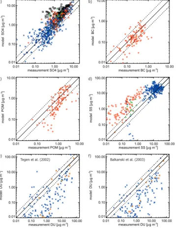
3.3. Mass distribution

As for budgets and lifetime, the mass distributions of the internally-mixed components are coherent. Figure2shows the annual mean vertically integrated aerosol mass (bur-den) for each component as sum over the modes. The maxima of the sulfate burden

15

lie close to the sources of sulfate and its precursors in the polluted regions of the north-ern hemisphere. However, substantial export of sulfate occurs to low emission regions such as the Middle East and northern Africa, the North Atlantic, and the North Pa-cific. The pronounced export to the Middle East and northern Africa seems facilitated

by the usage of the interactive dry deposition scheme. As described in Ganzeveld

20

et al. (1998), it calculates lower dry deposition velocities for SO₂ in that region than prescribed in many other studies, resulting in higher sulfate precursor concentrations. Additionally, the consideration of low roughness velocities over bare soils also results in low aerosol dry deposition, which is a major sink in that region, characterised by low precipitation. The burden of dust shows a distinct maximum extending from the

north-25

(26)

ACPD

4, 5551–5623, 2004

P. Stier et al.

Title Page

Tables Figures

◭ ◮

Back Close

Full Screen / Esc

Print Version

©EGU 2004

high over secondary source regions. The reason is that the storm tracks coincide with the strongest sink regions due to the associated precipitation. Therefore, regions such as the subtropical bands show, despite lower emissions, considerable column burdens of sea salt. Also shown is the burden of the total diagnosed aerosol water. From comparison with the distribution of the other compounds, it becomes evident that the

5

dominant fraction of aerosol water is associated with sea salt. However, over regions with high sulfate burden the uptake by sulfate is discernible.

To evaluate the simulated mass distributions, we compare the modelled aerosol mass concentration of the lowest model level with surface measurements for the

year 2000 from the European EMEP (http://www.emep.int) and North-American

IM-10

PROVE (http://vista.cira.colostate.edu/improve/) measurement networks as well as

to measurements compiled by the Global Atmosphere Watch (GAW) program (http:

//ies.jrc.cec.eu.int/wdca/). As most of these stations are at continental sites, we also include the comparison with a climatological compilation of multi-annual measurements at remote marine sites by courtesy of J. Prospero and D. Savoie (University of Miami),

15

henceforth denoted as University of Miami compilation.

To ensure comparability, stations deviating in height by more than 200 m from the lowest model level are rejected. For the year 2000 measurements from the EMEP, IMPROVE, and GAW networks, we sample the daily mean model output with the mea-surement occurrences, i.e. we include only days with meamea-surements in the derivation

20

of the model monthly mean values. Monthly means derived from less than 6 measure-ments are rejected. For the University of Miami dataset no information on the mea-surement dates and number of meamea-surements is available. Thus we use the whole model monthly mean for the comparison. A list of the measurement locations, with corresponding model and measurement annual mean and standard deviation, and the

25

total number of measurements can be found in Tables6–10). Figure3shows scatter-plots for the observed and simulated monthly mean surface mass concentrations for the di_fferent networks.

(27)

ACPD

4, 5551–5623, 2004

P. Stier et al.

Title Page

Tables Figures

◭ ◮

Back Close

Full Screen / Esc

Print Version

©EGU 2004

shows a good agreement with a slight tendency to overestimate. Out of a total of 112 samples, 74 (66%) agree within a factor of 2 with the measurements. In com-parison with the EMEP stations, distributed over Europe, the overestimation is more pronounced. However, still 182 (64%) out of 283 samples lie within a factor of 2. SU mass concentrations agree well with the GAW (7 (58%) out of 12) and University of

5

Miami compilations (196 (58%) out of 336).

For BC, measurements are only available from the North American IMPROVE net-work. The simulated surface BC masses show a good agreement with the measure-ments. Out of a total of 115 samples, 75 (65%) agree within a factor of 2. Considering the uncertainties associated with the SOA formation, the agreement for POM with 62

10

out of 115 samples (54%) within a factor of 2, is remarkable.

SS mass concentrations compare well with the remote marine measurements of the University of Miami dataset (181 (63%) out of 288 samples lie within a factor of 2 with the measurements) with a slight positive bias. Three measurement sites with excep-tionally high SS concentrations have been rejected as they are likely contaminated by

15

local surf (Savoie, pers. comm.). For the predominantly continental measurement sites from the IMPROVE and GAW networks, the low SS concentrations are substantially overestimated by the model, so that only 5 samples (4%) out of 113 for IMPROVE and 3 samples (25%) out of 12 for GAW agree within a factor of 2 with the measurements. This overestimation can possibly be attributed to numerical di_ffusion associated with

20

the strong gradients of sea salt along the coast lines.

For the seasonal and inter-annual highly variable dust cycle, the comparison with the climatological University of Miami data set shows a large scatter and low agreement for both, theTegen et al. (2002) and the Balkanski et al. (2003) emission schemes. Generally, the predicted mass concentrations are underestimated, a fact that is

par-25

(28)

ACPD

4, 5551–5623, 2004

P. Stier et al.

Title Page

Tables Figures

◭ ◮

Back Close

Full Screen / Esc

Print Version

©EGU 2004

than the lower background concentrations responsible for a large part of the scatter. It has to be stressed that in a comparison of a one year simulation with a climatological

dataset a not too good agreement can be expected. Further, as shown byTimmreck

and Schulz (2004) based on a study with the ECHAM4 GCM and theBalkanski et al.

(2003) emission scheme, the application of the nuding technique influences the wind

5

statistics and spatial distribution, substantially reducing the dust emissions. Other po-tential explanations include: the neglect of the super-coarse mode emissions, a too low emission strength particularly of the Asian dust sources dominating a large part of the Pacific measurement sites, an overestimation of sink processes, possibly due to too efficient microphysical aging, as well as the influence of non-represented local sources

10

on the dust measurements.

3.4. Number distribution

The annual-mean zonal-mean aerosol number concentration (N) for the seven modes is shown in Fig.4. Nucleation is favoured in regions with little available aerosol surface area, low temperatures, and high relative humidity. Thus, the maxima of the nucleation

15

mode number concentration can be found in the upper tropical troposphere and in the remote regions of the Antarctic where convective detrainment and DMS conversion, respectively, provide su_fficient sulfuric acid. Note that a large part of the nucleation mode particles have radii below the typical detection limit of 3 nm of current measure-ment techniques. Number concentrations of the insoluble Aitken mode are determined

20

by primary emissions of BC and POM and therefore highest in the lower troposphere close to the source regions of biomass burning and anthropogenic emissions. The sol-uble Aitken mode numbers are dominated by particles growing from the nucleation in the Aitken size-range. Accumulation and coarse insoluble modes are externally mixed dust modes and reflect the zonal distribution of the dust emissions, with the largest

25

(29)

ACPD

4, 5551–5623, 2004

P. Stier et al.

Title Page

Tables Figures

◭ ◮

Back Close

Full Screen / Esc

Print Version

©EGU 2004

found in the upper troposphere, attributable to convective detrainment of particles and their precursors. Coarse mode soluble particles are mainly confined to the lower tropo-sphere and can mostly be attributed to sea salt emissions. Between 15◦ N and 20◦N a local maximum due to the contribution of aged dust particles is identifiable around 800 hPa.

5

To evaluate the simulated aerosol number concentrations, we compare them in Fig.5

to vertical profiles obtained from aircraft measurements of the German Aerospace Agency (DLR), by courtesy of Petzold and Minikin (in preparation). The measure-ments were conducted during the “Interhemispheric di_fferences in cirrus properties from anthropogenic emissions” (INCA,http://www.pa.op.dlr.de/inca/) experiments and

10

the UFA2/EXPORT campaign in the year 2000. To avoid ambiguities in the compari-son with individual flight data, we compare campaign mean and median profiles of the simulation with campaign mean and median profiles of the measurements. The model data is averaged over the grid boxes containing the measurement domain. The model aerosol numbers are the superposition of the individual modes of HAM folded with the

15

cut-offof the measurement instruments.

The first INCA campaign was conducted in southern Chile (INCA-SH) from (23 March 2000–14 April 2000) in the domain (83.9◦W–69.1◦W, 58.5◦S–51.0◦S). The measured profile of aerosol numbers shows distinct maxima of median and mean in the mid-troposphere, between 2 and 7 km. ECHAM5-HAM well reproduces the

20

vertical distribution of aerosol numbers. The underestimation in the lower boundary layer can be attributed to an underestimation of nucleation. The second INCA cam-paign was conducted in Scotland (INCA-NH) from 27 September 2000–12 October 2000) in the domain (8.7◦W–3.6◦E, 54.6◦N–61.2◦N). The median particle concentra-tion shows a homogeneous distribuconcentra-tion throughout the troposphere and is well

cap-25

(30)

con-ACPD

4, 5551–5623, 2004

P. Stier et al.

Title Page

Tables Figures

◭ ◮

Back Close

Full Screen / Esc

Print Version

©EGU 2004

tinental Europe were obtained during the UFA2/EXPORT campaign (19 July 2000–10 August 2000) in the domain (5.3◦E–28.8◦E, 43.5◦N–56.7◦N). The observedN shows a distinct maximum in the boundary layer, a mid tropospheric minimum around 5 km, and a second maximum between 7 and 11 km. The ECHAM5-HAM simulated profile ofN is in good agreement with the observations throughout most of the troposphere.

5

However, the aerosol numbers in the lower boundary layer are under-predicted. Possi-ble explanations are a too efficient growth into larger size regimes, a too large emission size-distribution, underestimation of the emissions, or overestimated surface sinks. It has to be pointed out that as no simultaneous measurements of aerosol mass are available, it is not possible to further isolate one of those causes.

10

The simulated variability ofN, in terms of the di_fference of the 90thpercentile (P90)

and the 10th percentile (P10), for the polluted cases of UFA-EXPORT and INCA-NH

is lower than in the measurements. In addition to the ambiguity of the comparison of grid-box mean values with local measurements, one explanation could be the usage of monthly mean emission data. The variability for the maritime southern hemispheric

15

case INCA-SH, where interactively calculated natural emissions dominate, agrees well with the observations.

3.5. Radiative properties

Unlike the spatiotemporally constrained in-situ measurements, remote sensing data from satellites, supplemented by ground-based remote sensing, allows evaluation the

20

model on a global scale. As the input parameters for the ECHAM5 radiation scheme are calculated by HAM explicitly in dependence of the size-distribution and composi-tion of the modes, the resulting optical properties provide integrated informacomposi-tion on the model performance. However, it should be kept in mind that remote sensing retrievals have uncertainties and maybe biased, in particular satellite retrievals of aerosol

prop-25

erties over land. Therefore, differences between model results and remote sensing products do not necessarily reflect model deficiencies.

(31)

ACPD

4, 5551–5623, 2004

P. Stier et al.

Title Page

Tables Figures

◭ ◮

Back Close

Full Screen / Esc

Print Version

©EGU 2004

displayed in Fig. 6a. The regions with highest values of the simulated AOD are the Saharan dust plume extending into the Atlantic, biomass burning regions of Cen-tral Africa, and Asian regions with strong anthropogenic contributions, particularly regions over China and India. The simulated global annual mean optical depth at 0.14 falls in the range suggested by other global models (0.116–0.155) participating

5

in the AEROCOM model inter-comparison (http://nansen.ipsl.jussieu.fr/AEROCOM/). The ECHAM5-HAM mean value is almost identical to a sampling bias corrected global average of AERONET (Kinne et al., in preparation) of 0.14. A similar corrected global annual average of the best available global data set, even so without coverage at high latitudes, a MODIS-MISR composite (see below), suggests a slightly larger value of

10

about 0.16. This agreement is encouraging in light of the many retrieval uncertainties and the likelihood of AOD overestimates due to errors in cloud-screening. While, a good quantitative agreement to data on a global annual basis is encouraging, matches for distribution pattern on a regional and seasonal are a more meaningful test.

In comparisons to AOD simulations of Fig. 6a, a measurement based AOD

com-15

posite derived from advanced satellite retrievals is presented in Fig.6b. This data-set comprises a composite of monthly means based on satellite retrievals between March 2000 and February 2001. It combines the strength of di_fferent retrievals applied to multi-spectral data of the MODIS and MISR sensors on NASA’s EOS TERRA platform: Over water, data of the MODIS ocean retrieval (Tanr ´e et al., 1997) are used, while

20

over land the multi-directional retrieval of MISR (Martonchik et al.,2002), when avail-able, is preferred over the MODIS land retrieval (Kaufman et al.,1997). MODIS and MISR derived aerosol properties were validated against AERONET sun-photometer measurements. AOD retrieval errors are estimated at_±0.04 (at 10 km scales) for the MODIS ocean retrieval (Remer et al., 2002) and at _±0.05 (at 50 km scales) for the

25