STANDALONE TERRESTRIAL LASER SCANNING FOR EFFICIENTLY CAPTURING AEC BUILDINGS FOR AS-BUILT BIM

STANDALONE TERRESTRIAL LASER SCANNING FOR EFFICIENTLY CAPTURING

AEC BUILDINGS FOR AS-BUILT BIM

M. Bassier∗_{, M. Vergauwen, B. Van Genechten}

Dept. of Civil Engineering, TC Construction - Geomatics KU Leuven - Faculty of Engineering Technology

Ghent, Belgium

(maarten.bassier, maarten.vergauwen, bjorn.vangenechten)@kuleuven.be

Youth Forum

KEY WORDS:Scan to BIM, Terrestrial Laser scanning, Building, as-built BIM, AEC industry

ABSTRACT:

With the increasing popularity of as-built building models for the architectural, engineering and construction (AEC) industry, the demand for highly accurate and dense point cloud data is rising. The current data acquisition methods are labour intensive and time consuming. In order to compete with indoor mobile mapping systems (IMMS), surveyors are now opting to use terrestrial laser scanning as a standalone solution. However, there is uncertainty about the accuracy of this approach. The emphasis of this paper is to determine the scope for which terrestrial laser scanners can be used without additional control. Multiple real life test cases are evaluated in order to identify the boundaries of this technique. Furthermore, this research presents a mathematical prediction model that provides an indication of the data accuracy given the project dimensions. This will enable surveyors to make informed discussions about the employability of terrestrial laser scanning without additional control in mid to large-scale projects.

1. INTRODUCTION

The use of semantic three dimensional data models like Build-ing Information ModellBuild-ing (BIM) is becomBuild-ing more popular in the architectural, engineering and construction (AEC) industry. With no available models for existing buildings, the demand for accurate as-built models is also increasing. In the AEC industry, BIM is used for asset management, project planning, refurbish-ment and other purposes. As-built models require a certain level of accuracy (LOA) and a level of detail (LOD). The U.S. Federal Geographic Data Committee specifies that, in terms of geometry, LOA30 is recommended for AEC industry buildings (F.G.D.C, 2002). For detailing, LOD300 is accepted for most applications (BIMFORUM, 2013). In order to meet these requirements, highly accurate and dense point cloud data is needed. The current work flow, employing a terrestrial laser scanner and a total station, is costly and time consuming (D. Backes, C. Thomson, 2014). In order to compete with indoor mobile mapping systems (IMMS), surveyors are now opting to use their terrestrial laser scanners as a standalone solution. However, there is uncertainty about whether or not projects are still within specifications without a traditional control network.

The emphasis of this paper is to investigate the scope for which terrestrial laser scanners can be used without additional control of total stations. Furthermore, this research will also provide a mathematical prediction model to determine the feasibility of this approach for future projects. The rest of this article is organized as followed. Subsections 1.1, 1.2 and 1.3 review the scope of the intended projects and the process from reality to a registered point cloud. A section of related work is found in section 2. Our methodology is presented in section 3. The different test cases are described in section 4. The results and the calculated prediction model are shown in section 5. The discussion and future work are discussed in section 6. Finally, the conclusions are presented in section 7.

∗_{Corresponding author}

1.1 AEC buildings

The focus of this research is on the data acquisition of AEC build-ings e.g. airports, hospitals, office buildbuild-ings, schools, etc. These buildings consist of multiple structures, with several floors, cov-ering tens of thousands of square meters of useful space. Bosch´e (Bosch´e, 2012) describes how the AEC context has both advan-tages and constraints for the acquisition of point cloud data.

Large scale AEC sites generally tend to be very large. Also, both indoor and outdoor measurements should be acquired. Fur-thermore, depending on the project, ranges can vary from me-ters to tens of meme-ters. This proves problematic for most IMMS since drift is accumulated over time, instrument ranges are lim-ited and sunlight interference can cause signal disturbance. Also, the amount of data generated is enormous, causing problems in data processing and storage.

Occlusion Terrestrial laser scanning and other LIght Detection And Ranging (LIDAR) technologies can only capture points in line of sight. While most data occlusion can be avoided by the sensors position, occluded zones caused by fake ceilings, built-in closets, inaccessible areas, etc. cannot be avoided. Both mod-ellers and algorithms are forced to make assumptions about these zones, which often lead to misinterpretation.

Self-similarities AEC buildings tend towards self-similarity a-cross different rooms and floors. Bosch´e (Bosch´e, 2012) states that these resemblances present a challenging constraint for the registration process. Therefore, Simultaneous Localization And Mapping (SLAM) or automatic registration algorithms are prone to misalignment in these environments.

1.2 Data acquisition

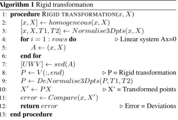
Algorithm 1Rigid transformation

1: procedureRIGID TRANSFORMATION(x, X) 2: [x, X]←homogeneous(x, X)

3: [x, X, T1, T2]←N ormalise3Dpts(x, X)

4: fori= 1 :rowsdo ⊲Linear system Ax=0

5: A←(x, X) 6: end for

7: [U W V]←svd(A)

8: P ←V(:, end) ⊲P = Rigid transformation 9: P ←DeN ormalise3Dpts(P, T1, T2)

10: X′_{←P X ⊲X’ = Transformed points}

11: error←Compare(x, X′₎

12: returnerror ⊲Error = Deviations

13: end procedure

is pushed, carried, driven or flown trough the structure. These in-struments are characterized by their continuous movement and data capture. With their superior speed, these systems are de-signed to capture the scene in a minimum amount of time. How-ever, the dynamic approach is prone to drift and noise, which results in less accurate point clouds. Thomson et al (Thomson et al., 2013) concluded that despite the enormous time savings, these systems do not perform adequately for high accuracy appli-cations. Bosse et al (Bosse et al., 2012) and Zlot et al (Zlot et al., 2013) confirm that hand held mobile devices like the ZEB1 are only fit for low accuracy applications. Trolley based systems from Viametris, Navvis or Trimble show better results, yet lack the accuracy to provide LOA30 (Viametris, 2007, NavVis, 2013, Trimble, 2012).

Static systems mount their sensors on a non-mobile platform and utilise a stop-and-go approach to capture the scene. Currently, the most popular static instrument for the acquisition of point cloud data is a terrestrial laser scanner. The system provides fast and reliable point measurements in a 360◦_{field of view. Furthermore,} terrestrial laser scanners can measure up to several hundreds of meters and can be utilised in most environment conditions. The result is a geometric point cloud containing tens of millions of points with high accuracy.

For as-built surveying, a terrestrial laser scanner is commonly utilised to meet the specified LOA. Placed on a tripod, the strument is used to create scans on multiple locations. The in-dividual point clouds are tied together using artificial targets or cloud to cloud constraints. In addition, targets spread throughout the scene are also measured with a total station to establish survey control. While this work flow is highly accurate, it is a costly and time consuming process (D. Backes, C. Thomson, 2014). The use of total stations is a driving cost in this process: These instru-ments are slow, require skilled personnel and provide only sparse data unfit for as-built conditions.

1.3 Data processing

There are two main approaches to align scan data. Target-based registration is based on the matching of artificial targets spread throughout the scene. Cloud-based registration uses features ex-tracted from the data itself. Both registrations follow the same process which consists of two steps: A coarse alignment gives an initial approximation of the relative positioning, which is fol-lowed by a fine alignment that enhances the registration (Bosch´e, 2012). Both processes are well studied problems. Several solu-tions have been presented on the coarse alignment of the cloud-based registration. Jaw (Jaw and Chuang, 2008) proposes a fea-ture based approach using points as landmarks, while Akca () and Hansen (Hansen, 2007) focus on surface based registration.

Recently, curves have also been used for the process by Yang (Yang and Zang, 2014). The fine registration usually is performed using some variant of the iterative closest point algorithm (ICP) (Besl and McKay, 1992, Chetverikov et al., 2002, Minguez et al., 2006). Given a good initial alignment, these algorithms are able to converge to an optimal solution. However, the solution is de-pendant on the data. In the case of erroneous data, the registration will provide a false alignment. As more clouds are added to the registration, these errors can cause critical damage to the overall accuracy.

2. RELATED WORK

Several researchers have published findings on data acquisition solutions for building modelling. Generally, the emphasis is on indoor mobile mapping. While many approaches have proven successful, most solutions are limited to small scale data (e.g. a hallway, a room, etc.). One of the most prominent publica-tions has been the comparison of IMMS compared to Terrestrial laser scanning (TLS) in terms of accuracy and acquisition speed (Thomson et al., 2013). In this research, both the IMMS of Vi-ametris (ViVi-ametris, 2007) and the ZEB1 from CSIRO (Bosch´e, 2012) are discussed. Thomson et al concludes that IMMS might have a significant impact on future workflows, but currently lack sufficient accuracy. Also, the University College London (UCL) presented a report with the test case of a Scan-to-BIM project (D. Backes, C. Thomson, 2014). Data acquisition was performed using a terrestrial laser scanner along with total station measure-ments. Their research concluded that traditional survey work-flows were inefficient and that IMMS might provide a solution. Several other papers have been presented on the ZEB1, describ-ing the system as a solution for low accuracy applications (Bosse et al., 2012, Zlot et al., 2013). Similar to the Viametris, findings have been reported for several other trolley based systems (Vi-ametris, 2007, NavVis, 2013, Trimble, 2012). Another solution is the integration of several 2D laser scanners and other sensors in a backpack, providing a fast and hands free approach (Liu and Wang, 2010). Other LIght Detection And Ranging (LIDAR) in-tegrated approaches have similar results (Tang et al., 2010). A lot of research is being performed on the integration of RGB-D cameras like the Microsoft Kinect for indoor mapping (Whe-lan et al., 2013, Steinbr et al., n.d., Pirovano, 2012, Du et al., 2011, Yue et al., 2014, Liu and Wang, 2010). While projects like Google Tango (Google, 2014), Kintineous (Whelan et al., 2013) and Kinfu (Pirovano, 2012) succeed in mapping larger ar-eas, the integrated sensors lack the accuracy and range for build-ing mappbuild-ing. Photogrammetric approaches are bebuild-ing explored as well, but generally require additional geometric information (Furukawa et al., 2009).

3. METHODOLOGY

In this paper we seek to evaluate to which extend terrestrial laser scanning can be employed for the data acquisition of existing

Acquisition Processing Dimensions Shape Time [h] Time [h] X[m] Y[m] Z[m]

PVPO 4 7 70 40 4

F-pier 12 21 260 120 4

C-pier V1 15 33 250 100 4

C-pier V0 17 40 250 100 10

Table 1: Test site specifications

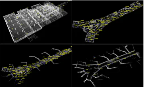
Figure 1: Overview control points: PVPO (Top left), F-pier (Top right), C-pier V1 (Bottom left) and C-pier V0 (Bottom right). The yellow dots indicate the location of the control points.

buildings without total station measurements. To that end, sev-eral real life test cases are treated in the same methodological manner: Each test site is scanned with a terrestrial laser scanner, and a control network is realized independently using total sta-tion measurements. The scan data is processed and the results are compared to the control network to assess the accuracy.

The comparison is performed as follows: After registering the scans, candidate targets are extracted from the point cloud using a statistical extraction tool in Leica Cyclone. The results are eval-uated using a least squares algorithm seen in Algorithm 1. The input for this algorithm consists of a set of control targets from the total station networkx={x1, x2, . . . xn}and a set of

candi-date targets from the point cloudX ={X1, X2, . . . Xn}. First,

the homogeneous coordinates of the 3D points are normalized with a linear conditioning transformation for numerical stability. Second, a best fit linear transformation is computed between the two data sets. Finally, the candidate targets are transformed and the residual 3D error with respect to the control measurements is computed. From these residuals we can construct a prediction model to determine the maximum project size for a given required accuracy.

4. TEST DESIGN

In order to acquire reliable results about the scope of terrestrial laser scanning in real life test cases, four test cases are evaluated. The tests were conducted using a phase-based FARO Focus3D S120 scanner, set in an arbitrary coordinate system. All scans were taken with 5-10m spacing at 12.5mm/10m resolution with the lowest quality. Given this resolution, point cloud vertices can be extracted from the cloud with a standard deviation of 2mm. The control network was established by an external surveying company which provides an accuracy of 2mm in each direction on every control point. The individual point clouds were regis-tered using Leica Cyclone 8.0. The registration software allows for cloud-based registration and the distribution of weights across its registration network.

Test sites Table 1 shows the four test cases and their specifi-cations. The first test site is located in the east passage of the central station in Amsterdam and has a rectangular shape. The three other test sites are located in the Schiphol International Air-port of the Netherlands. These test sites have varying dimensions

and are all y-shaped. C-pier V0 is a point cloud acquired along the exterior of the C-pier building. C-pier V1 consists of the en-tire interior of the first floor. The F-pier is similar to the C-pier V1. An overview of the point clouds and the control points can be seen in figure 1. All cases are acquired in real life conditions: Scenes are cluttered with furniture and people, there are highly reflective and glass objects present, the project geometry is not ideal, etc.

5. EXPERIMENTAL RESULTS

5.1 Data acquisition and Processing

The average data acquisition time with the FARO scanner varies between 22 and 24 scans an hour, depending on the project. The relation between data acquisition time and the number of scans is close to linear. The processing time however, is not: processing hours vary from 10 to 14 scans an hour and the time increases in relation to the number of scans. Several reasons can be found for the exponential growth of the processing time. First, the auto-mated cloud constraint algorithm embedded in the software eval-uates every possible constraint in the network. Therefore, the combinatoric complexity increases rapidly. For example, a 400 node network already considers 79,900 possible constraints. Sec-ond, the number of scans has a direct impact on the file size. As the amount of data grows, the data becomes increasingly more difficult to work with.

5.2 Cloud registration

The results of the cloud-based registration are shown in table 2. The Cyclone software provides two parameters that give an indi-cation of the registration accuracy.

Point clouds Cloud constraints Mean error vector [m]

Std dev. error vector [m]

Mean error [m]

Std dev. error [m]

PVPO 98 1400 0.013 0.003 0.001 0.001

F-pier 290 3200 0.009 0.001 0.001 0.001

C-pier V1 365 3900 0.009 0.001 0.001 0.001

C-pier V0 422 4900 0.007 0.002 0.001 0.001

Table 2: Registration diagnostics

Control points

Point error

<1.5 cm

RMSE X [m] RMSE Y [m] RMSE Z [m]

PVPO 29 100 % 0.002 0.002 0.005

F-pier 56 66 % 0.002 0.002 0.034

C-pier V1 44 75 % 0.004 0.003 0.024

C-pier V0 12 66 % 0.005 0.004 0.017

Table 3: Control point comparison diagnostics

Error The error represents the displacement of each scan after network optimization in respect to their initial constraint. Table 2 reveals that in all test cases, the average error on the location of the final scan position is only 1mm. Given that every cloud is averagely linked by 15 constraints, the registration is highly reliable.

5.3 Point comparison

The point comparison is performed using algorithm 1. The point cloud vertices are statistically extracted from the registered point cloud using the Cyclone software. These points will serve as the candidate group while the control points will serve as a bench-mark. Both data sets consistently have an accuracy of 2mm. The results of the point cloud comparison is shown in table 3. The mean error for all projects is near zero due to the best fit rigid transformation of the datasets. In order to be sufficiently accu-rate, all points should have a root mean squared error lower than 1.5cm in all directions. Table 3 reveals that only in the case of the PVPO project, all errors are within LOA30 specification. In the other test cases, some errors exceed 1.5cm, and thus, addi-tional control is required for these projects. Therefore, the scope for which terrestrial laser scanning can be used in somewhere in between 100-300 scans. In Section 5.5, a more precise number of scans is derived using prediction models.

However, looking at the errors in the different direction, it is re-vealed that not all errors relate similarly to the amount of scans captured. For instance, both the error in X and Y direction are significantly smaller than the error in Z-direction. The root mean squared error in X and Y-direction for the PVPO and the F-pier is even in range of the benchmark accuracy. In addition, the devia-tions in X and Y direction seem to grow linearly while the error in Z-direction indicates a more quadratic error propagation. In sec-tion 5.4, several explanasec-tions are presented for this phenomenon.

5.4 Deviation analysis

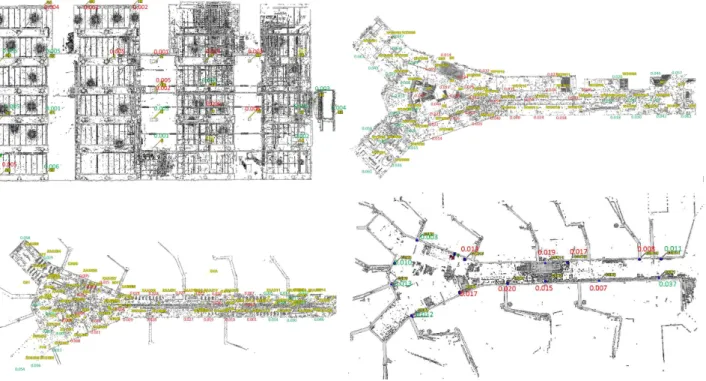
Considering the error across the different test cases, the devi-ations in all directions increase with increasing project dimen-sions. However, the error in Z-direction seems to be of a quadratic nature. With ICP algorithms (Besl and McKay, 1992) indepen-dent of any direction, the cause of this error is located in the data itself. Figure 2 plots the deviations in Z-direction on their re-spective locations for all sites. Across the different test cases, it is revealed that the red values concentrate in the centre, while the green values are located near the edges. These observations show that the project is bending upwards. The increasing error over consecutive scans suggest a systematic error is present. The impact of these errors is determined relating the errors in the Z-direction to the project dimensions for every test case. Given the

mean errors at varying sections, a deviation model can be calcu-lated for each project. Given the nature of the errors, a quadratic function is best fitted on the data using a least squares approach. Figure 3 depicts the deviation model for the different test cases.

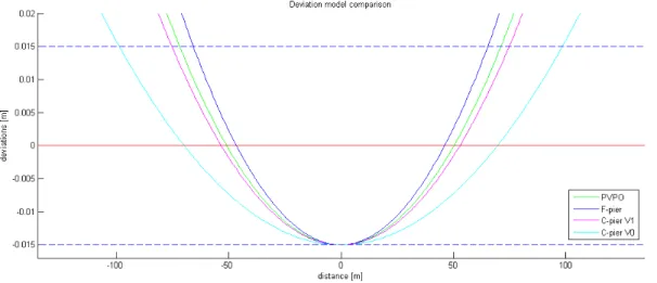
5.5 Error prediction model

To maximize efficiency, it is crucial to know when additional con-trol is required in a project. Therefore, the deviations in future projects should be predicted as accurately as possible. Using the known test cases, an error prediction model can be calculated to determine whether or not a project will meet the specified accu-racy. In regard to the LOA30 specification, the deviation models for each project can be reshaped to match the maximum error allowed. In figure 4 every model is realigned to the specified ac-curacy of 0.015m. Comparing the prediction errors, it is revealed that the models do not align. This causes the predicted error to ex-ceed LOA30 at varying project dimensions for the different test cases. The differences can be caused by project geometry, the amount of scans taken, the tightness of the network, the device, etc. For instance, while the F-pier has approximately the same dimensions as both C-pier sites, the reduced amount of scans in-creases the uncertainty. To determine the key factor that impacts the bending angle, figure 4 is analysed. There, a major discrep-ancy can be found between the C-pier V0 curve and the other three curves. Therefore, the answer must lie in the discrepancy of parameters between interior data sets (PVPO, F-pier, C-pier V1) and exterior data set (C-pier V0). One major difference is the data distribution in the Z-direction: The interior data sets have a data distribution in Z-direction of only 4m, while the exterior data set has a distribution of nearly 10m. The lack of distribution of the data can introduce critical errors in registration processes. This explanation is supported by the observation in X and Y-direction, where the errors show a more consistent pattern.

Given these prediction models, an estimation can be made for future projects. E.g. most office buildings have a floor height between three and four meters. Looking at the deviation model, it is estimated that project bending will exceed 1.5cm after ap-proximately 150m. Therefore, roughly 22,000m2_{can be scanned}

before any control should be added to meet LOA30.

6. DISCUSSION & FUTURE WORK

As previously stated, the cause of the project bending is system-atic in nature. Since it is located in the data itself, standard ICP algorithms cannot cope with this error. However, certain mea-sures can be taken to limit the impact of this error on the final point cloud. First, the data quality should be maximised. With

Figure 2: Overview deviations in the Z-direction per control point: PVPO (Top left), F-pier (Top right), C-pier V1 (Bottom left) and C-pier V0 (Bottom right). The values depicted in green indicate that the vertices are above the control points. The values in red indicate that the vertices are below the control points.

Figure 4: Error prediction model: All deviation models are realigned to fit the maximum allowed error in LOA30. The stripped blue lines indicates LOA30 boundaries. The quadratic curves depict the bending curves for each project.

more accurate and dense data, less uncertainty will be introduced to the registration. In this case, terrestrial laser scanners have the edge over IMMS with their superior data quality. Second, registration algorithms can be forced to lock the vertical angle of individual scans. Utilising a dual-axis compensator or inclinome-ter, the exact angle of each scan can be determined independently. In the registration process, these additional measurements can be used to adjust the scan locations. Therefore, employing scanners equipped with accurate levelling sensors and software that allow the required angle adjustments, can provide a solution to further extend our approach. Future work is being conducted on the in-tegration of this data in the registration process.

7. CONCLUSION

In this paper, we present a method to efficiently map AEC in-dustry buildings with only a Terrestrial Laser Scanner as a stan-dalone solution. Employing cloud-based registration, we are able to discard the use of total station measurements for mid-to-large scale buildings. Our experiments prove that this technology can be used without additional control in projects containing several hundreds of scans. The scope for which the approach can be used in Scan-to-BIM, can be determined by our prediction mod-els. Given the project dimensions, the deviation error in all direc-tions can be estimated. The error in X and Y-direction is linear and grows gradually over the amount of scans acquired. How-ever, the error in Z-direction grows quadratically, thus being the decisive factor in the point cloud accuracy. The experimental data shows that the data distribution in Z-direction is a major factor in the bending error. While these errors are small in individual scans, they can cause critical damage in large projects. The use of more accurate data and the adjustment of the vertical angle of the individual scans provide a possible solution to further extend our approach.

REFERENCES

Akca, D., 2007.Least Squares 3D Surface Matching.

Besl, P. and McKay, N., 1992. A Method for Registration of 3-D Shapes.

BIMFORUM, 2013. Level of development specification version 2013. pp. 0–124.

Bosch´e, F., 2012. Plane-based registration of construction laser scans with 3D/4D building models.Advanced Engineering Infor-matics26(1), pp. 90–102.

Bosse, M., Zlot, R. and Flick, P., 2012. Zebedee: Design of a spring-mounted 3-d range sensor with application to mobile map-ping.Robotics, IEEE Transactions onXX(Xx), pp. 1–15.

Chetverikov, D., Svirko, D., Stepanov, D. and Krsek, P., 2002. The Trimmed Iterative Closest Point algorithm. Object recogni-tion supported by user interacrecogni-tion for service robots3(c), pp. 0–3.

D. Backes, C. Thomson, D. J. B., 2014. Chadwick GreenBIM. Technical report.

Du, H., Henry, P., Ren, X., Cheng, M., Goldman, D. B., Seitz, S. M. and Fox, D., 2011. Interactive 3D modeling of indoor en-vironments with a consumer depth camera. Proceedings of the 13th international conference on Ubiquitous computing - Ubi-Comp ’11p. 75.

F.G.D.C, 2002. Geospatial Positioning Accuracy Standards PART 4 : Standards for Architecture , Engineering , Construc-tion ( A / E / C ) and Facility Management.

Furukawa, Y., Curless, B., Seitz, S. M. and Szeliski, R., 2009. Reconstructing building interiors from images. 2009 IEEE 12th International Conference on Computer Vision(Iccv), pp. 80–87.

Google, 2014. Google project Tango.

Hansen, W. V., 2007. Registration of agia sanmarina lidar data using surface elements. pp. 1–6.

Jaw, J. J. and Chuang, T. Y., 2008. Feature-Based Registra-tion Of Terrestrial Lidar Point Clouds. ISPRS Commission III

XXXVII(3b), pp. 303–308.

Liu, S. and Wang, C. C., 2010. Orienting unorganized points for surface reconstruction. Computers & Graphics34(3), pp. 209– 218.

Minguez, J., Montesano, L. and Lamiraux, F., 2006. Metric-based iterative closest point scan matching for sensor dis-placement estimation. IEEE Transactions on Robotics22(5), pp. 1047–1054.

NavVis, 2013. NavVis 3D Mapping Trolley Specifications.

Pirovano, M., 2012. Kinfu an open source implementation of Kinect Fusion + case study : implementing a 3D scanner with PCL.

Steinbr, F., Kerl, C. and Cremers, D., n.d. Large-Scale Multi-Resolution Surface Reconstruction from RGB-D Sequences.

Tang, P., Huber, D., Akinci, B., Lipman, R. and Lytle, A., 2010. Automatic reconstruction of as-built building information models from laser-scanned point clouds: A review of related techniques.

Automation in Construction19(7), pp. 829–843.

Thomson, C., Apostolopoulos, G., Backes, D. and Boehm, J., 2013. Mobile Laser Scanning for Indoor Modelling. ISPRS An-nals of Photogrammetry, Remote Sensing and Spatial Informa-tion SciencesII-5/W2(November), pp. 289–293.

Trimble, 2012. TRIMBLE R10 GNSS System.

Viametris, 2007. indoor Mobile Mapping System The Freedom to map while in motion.

Whelan, T., Johannsson, H., Kaess, M., Leonard, J. J. and Mc-donald, J., 2013. Robust real-time visual odometry for dense RGB-D mapping.. . . (ICRA), 2013 IEEE . . ..

Yang, B. and Zang, Y., 2014. Automated registration of dense ter-restrial laser-scanning point clouds using curves. ISPRS Journal of Photogrammetry and Remote Sensing95, pp. 109–121.

Yue, H., Chen, W., Wu, X. and Liu, J., 2014. Fast 3D modeling in complex environments using a single Kinect sensor. Optics and Lasers in Engineering53, pp. 104–111.

Zlot, R., Bosse, M., Greenop, K., Jarzab, Z., Juckes, E. and Roberts, J., 2013. Efficiently capturing large, complex cultural heritage sites with a handheld mobile 3D laser mapping system.