Estimating the stochastic bifurcation structure of cellular networks.
Texto
Imagem
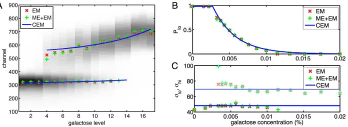
![Figure 2 displays the data, which is broadly consistent with previous experiments [25]](https://thumb-eu.123doks.com/thumbv2/123dok_br/18378915.356179/4.918.91.789.89.602/figure-displays-data-broadly-consistent-previous-experiments.webp)
Documentos relacionados
didático e resolva as listas de exercícios (disponíveis no Classroom) referentes às obras de Carlos Drummond de Andrade, João Guimarães Rosa, Machado de Assis,
Diretoria do Câmpus Avançado Xanxerê Rosângela Gonçalves Padilha Coelho da Cruz.. Chefia do Departamento de Administração do Câmpus Xanxerê Camila
The probability of attending school four our group of interest in this region increased by 6.5 percentage points after the expansion of the Bolsa Família program in 2007 and
No campo, os efeitos da seca e da privatiza- ção dos recursos recaíram principalmente sobre agricultores familiares, que mobilizaram as comunidades rurais organizadas e as agências
Há evidências que esta técnica, quando aplicada no músculo esquelético, induz uma resposta reflexa nomeada por reflexo vibração tônica (RVT), que se assemelha
não existe emissão esp Dntânea. De acordo com essa teoria, átomos excita- dos no vácuo não irradiam. Isso nos leva à idéia de que emissão espontânea está ligada à
Maria II et les acteurs en formation de l’Ecole Supérieure de Théâtre et Cinéma (ancien Conservatoire), en stage au TNDM II. Cet ensemble, intégrant des acteurs qui ne
i) A condutividade da matriz vítrea diminui com o aumento do tempo de tratamento térmico (Fig.. 241 pequena quantidade de cristais existentes na amostra já provoca um efeito
