Brazilian Journal of Physics, vol. 38 , no. 3B, September, 2008 499
Langevin Simulations with Colored Noise and Non-Markovian Dissipation
R. L. S. Farias, R. O. Ramos, and L. A. da Silva
Departamento de F´ısica Te´orica, Universidade do Estado do Rio de Janeiro, 20550-013 Rio de Janeiro, RJ, Brazil (Received on 14 April, 2008)
The nonequilibrium dynamics of an homogeneous scalar field is studied using Langevin equations. Micro-scopic derivations based on quantum field theory methods can lead to complicated nonlocal equations of motion. Here we study, numerically, the results obtained by appropriately approximating these equations in a local form (the Markovian approximation) and compare with results obtained with suitable prescriptions for accounting for the nonlocal terms,i.e.the non-Markovian form. We use a prescription for the nonlocal equations motivated by the results obtained from previous derivations using nonequilibrium quantum field theory methods.
Keywords: Langevin equation; Non-Markovian; Colored noise
1. INTRODUCTION
Nonequilibrium dynamics is expected to happen in many important physical problems. Systems of particular interest are in the physics of heavy-ion collisions, cosmology and con-densed matter physics. In the context of cosmology, we have interest in early universe scenarios. Nonequilibrium methods are being applied to get a quantitative understanding of the theory of reheating with the aim of explaining the change to radiation phase of the universe after inflation [1].
In the context of heavy-ion collisions, with the recent ex-periments in the RHIC concerning the possibility of forma-tion of a quark-gluon plasma [2], it is expected that the chiral fields should evolve under extreme conditions of temperature and energy density during the QCD phase transition and the out-equilibrium evolution for the fields becomes an important issue. To have a clear understanding of data coming from BNL-RHIC, and especially of data that will be produced at CERN-LHC, one needs a realistic description of the hierar-chy of scales associated with dissipation, noise and radiation. Also, the expansion and finite size of the system must be con-sidered. The study and understanding of all these processes mentioned above require the use of nonequilibrium quantum field theory methods [3].
In the context of condensed matter physics, many efforts have been devoted to get a better understanding of quantum many body dynamics, e.g in laboratory experiments of ultra-cold quantum Bose/Fermi gases [4]. One interesting question in that context is about the role of quantum fluctuations on the dynamics of scalar fields, which are usually neglected when we apply the classical field theory approximation given by the Gross-Pitaevskii equation [5].
Recently, a nonperturbative description of nonequilibrium quantum fields based on the two-particle irreducible (2PI) effective action formalism has proven very powerful with a wide range of applications [6]. In this work we study the nonequilibrium dynamics making use of numerical methods based on simulations of Langevin equations in a lattice. In our approach, the interaction with the environment is modeled by noise and dissipation terms and these terms are considered as local (Markovian) ones. However, microscopic derivations based on quantum field theory methods lead to complicated nonlocal equations of motion [7, 8].
Here, we study numerically the Langevin dynamics for an
homogeneousλφ4theory. Since there is an immense saving of
effort as well as much more transparent understanding of the physics from a local equation as opposed to a nonlocal one, since the former can generally be analyzed with much less numerical treatment than the latter, thus it is a very impor-tant question when and how accurately the generally nonlo-cal effective equations can be approximated by a lononlo-cal form. Numerical results from simulations for a specific model are shown here and the local (Markovian) and nonlocal (non-Markovian) equations are then compared for different region of parameters. We expect that these results and methods pre-sented here can be useful in the problems being considered in the context of the RHIC physics.
2. CLASSICAL LANGEVIN EQUATION
Typical stochastic evolution is well represented by the prob-lem of the classical brownian motion, whose properties can be represented by a phenomenological equation of the form
¨
φ(t) +ηφ˙(t) +V′(φ) =ξ(t), (1)
whereφ is a variable of the system (for example the coor-dinate of a particle) in interaction with a thermal bath, effec-tively modeled by a friction term, of intensityη, and stochastic noiseξ(t). The stochastic noiseξ(t), in its simplest realiza-tion, is considered as Gaussian and white and two-point cor-relation function given according to the classical Fluctuation-Dissipation theorem:
hξ(t)i=0, hξ(t)ξ¡
t′¢i=2Tηδ¡
t−t′¢. (2)
500 R. L. S. Farias, R. O. Ramos, and L. A. da Silva
3. THE NONLOCAL NOISE AND DISSIPATION KERNELS IN QUANTUM FIELD THEORY
In the realm of quantum field theory, explicit derivations of effective equations of motion for background fields (used for example in the determination of the dynamics of an or-der parameter in the theory, e.g. for studying phase transi-tions), show that the effective dynamics for fields are deter-mined by complicate integro-differential equations [7, 9, 10], where both dissipation and noise are determined by nonlocal (non-Markovian) kernels. This is exemplified by a result ob-tained in a scalar field theory with aλφ4interacting potential
and in a thermal bath at temperatureT. For an homogeneous field configuration, computed in a two-loop calculation in a quasi-particle approach for the scalar field propagators, it can be shown that the noise correlation function is found to be given by [7, 8]
ξ1(x,t)ξ1¡x′,t′¢®=K¡t−t′¢δ(x−x′), (3)
where
K¡ t−t′¢
= λ
2
2
Z d3q
(2π)3
e−2Γ(q)|t−t′|
4ω2(q)
n
2n(ω) [1+n(ω)] + £
1+2n(ω) +2n2(ω)¤ cos£
2ω|t−t′|¤ + 2βΓ(q)n(ω) [1+n(ω)] [1+2n(ω)]
× sin£2ω|t−t′|¤ o
, (4)
withn(ω) = [exp(βω)−1]−1 is the Bose-Einstein distribu-tion,β=1/T,ωis the dispersion relation given in terms of the momentumq≡ |q|andΓ(q)is the thermal decay width for the scalar fieldφ. Differently than the simplest Langevin equation, where noise is considered white (Markovian), like in Eq. (2), here, we see from Eq. (4) that noise is non-Markovian in time.
4. NON-MARKOVIAN EQUATION OF MOTION
Our goal is to simulate a non-Markovian Langevin-like equation of motion, whose noise kernel is in a form similar to Eq. (4). We consider an homogeneous scalar field configu-ration,φ≡φ(t), with equation of motion
¨
φ+V′(φ) + Z t
t0
dt′K(t−t′)φ˙(t′) =ξ(t), (5) wheret0is the initial time,
V′(φ) =Ω2 0φ+
λ 3!φ
3, (6)
and the nonlocal kernel is given by
K¡t−t′¢ = e−γ2(t−t′)QΩ
2 0 γ
n
cos£Ω1
¡
t−t′¢¤+
+ γ
2Ω1
sin£
Ω1¡t−t′¢¤
¾
, (7)
whereγ,QandΩ0are parameters andΩ21=Ω20−γ2/4>0.
In Eq. (5)ξ(t)is a non-Markovian Gaussian noise satisfy-ing
hξ(t)i=0, hξ(t)ξ(t′)i = T K(t−t′). (8) It can be easily shown that this noise can be generated by the following differential equation [11]:
¨
ξ(t) +γξ˙(t) +Ω2
0ξ(t) =Ω20
p
2T Qζ(t), (9) ζ(t)in Eq. (9) is a white Gaussian noise satisfying
hζ(t)i=0, hζ(t)ζ¡ t′¢
i = δ¡
t−t′¢
. (10)
It can be noted that the general solution of Eq. (9) is given by
ξ(t) = C1e−
γ
2tcos(Ω1t) +C2e−
γ
2tsin(Ω1t)
+ e
−γ2t
Ω1 Ω2
0
p 2QT
½·Z
dt′cos¡
Ω1t′¢
× ζ¡
t′¢e−γ2t′
i
sin(Ω1t)−
·Z
dt′′sin¡Ω1t′′
¢
× ζ¡
t′′¢ e−γ2t′′
i
cos(Ω1t)
o
. (11)
It can easily be shown that the stationary part of Eq. (11), when used to compute the two-point correlation function, gives the kernelK(t−t′), Eq. (7). We can then solve Eq. (9) numerically for some time so to assure to get the stationary solutions. After this time, we solve the remaining equations of the system altogether. To built this system of equations, it is useful to do the following tricks that allow us to write Eq. (5) in a completely local form. Firstly, we define two new variables,w(t)andu(t), given, respectively, by
w(t) =−
Z t
t0
dt′K(t−t′)φ˙(t′) +ξ(t), (12) and
u(t) = Z t
t0
dt′£K˙(t−t′)−γK(t−t′)¤˙
φ(t′), (13) where the time derivatives inside the time integral are (always) with respect tot′. After a little algebra, we find that the equa-tions of motion forwanduare
˙
w(t) =u(t)−γ[w(t)−ξ(t)]−K(0)φ˙(t) +ξ˙(t), (14) and
˙
u(t) =−Ω2
Brazilian Journal of Physics, vol. 38 , no. 3B, September, 2008 501
Putting Eqs. (5), (9), (14) and (15) together, we obtain a sixth order dynamical system that is completely local in time,
˙ φ = y,
˙
y = −V′(φ) +w, ˙
w = u−γ(w−ξ)−K(0)y+z, ˙
u = −Ω2
0(w−ξ) +K˙(0)y−γK(0)y,
˙ ξ = z,
˙
z = −γz−Ω2 0ξ+Ω20
p
2T Qζ. (16)
Therefore, starting with a non-Markovian Langevin like equa-tion of moequa-tion like Eq. (5), we are able to rewrite it in terms of a sixth order dynamical system of local equations, which are more feasible to treat numerically.
5. NUMERICAL RESULTS
We now show the results of our simulations for the time evolution of φ(t). Results can be presented for different choices of parameters. For example, we can show the re-sults varying the parameterγin the kernel (7), which sets the time scale for the thermal bath. Results can also be presented for different values of Ω0, the frequency of the system and
also chosen for the thermal bath, thus simulating the original derivation of Eq. (4), where the thermal bath was generated by the system own fluctuations. Since we want to more closely follow this last point of view, here we study the results for dif-ferent choices ofΩ0, chosen so as to mimic closely the results
e.g. of Ref. [7], and we also consider the cases whereT>Ω0,
again mimicking the derivation in that reference.
In Figs. 1-3 we show the numerical results coming from the simulation of the system of equations (16) forφ, obtained as an average over 100,000 realizations over the noise. The step size in time considered was 0.01. In all cases we checked for the numerical stability of the results. The results from the nonlocal equation of motion are then compared with the ones obtained in the local approximation, obtained from Eq. (1), withηdefined by
η≡
Z ∞
0
dtK(t) =Q, (17)
which corresponds to the local limit for the kernel given by Eq. (7). The initial conditions considered for all simulations wereξ(t0) =1, ˙ξ(t0) =0,φ(t0) =1, ˙φ(t0) =0,w(t0) =1 and
u(t0) =0. The interaction parameterλin Eq. (6) is chosen as λ=1.
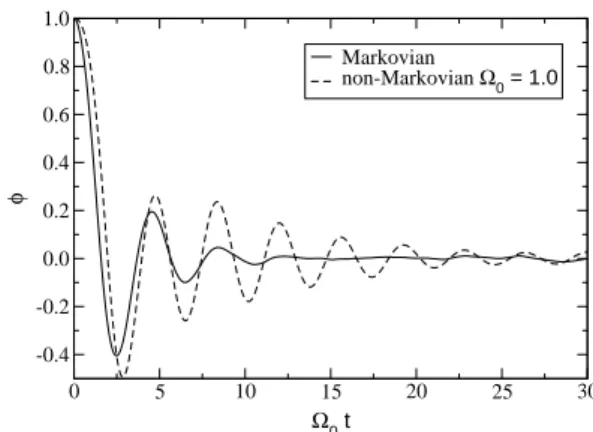
From the results shown in Figs. 1-3 we can notice that for values ofΩ0.1.5 the Markovian (local) approximation tends
to overestimate the dissipation in the system, while for values of Ω0&1.5 the local approximation tends to underestimate
the true dissipation as would come from the nonlocal kernel. These same figures also show that the larger isΩ0, the faster
is the thermalization of the system. This shows that asΩ0
in-creases, which is also associated to the frequency of the mem-ory kernel chosen, the larger is the fluctuations of the kernel,
0 5 10 15 20 25 30
Ω0 t
-0.4 -0.2 0.0 0.2 0.4 0.6 0.8 1.0
φ
Markovian
non-Markovian Ω0 = 1.0
FIG. 1: Time evolution for φ(t) in both Markovian and non-Markovian regimes andΩ0=1.0. The other parameters are taken asγ=1.0,Q=0.5,T=10.0 andλ=1.0.
0 5 10 15 20 25 30
Ω0 t
-0.5 0.0 0.5 1.0
φ
Markovian
non-Markovian Ω0 = 1.5
FIG. 2: Time evolution for φ(t) in both Markovian and non-Markovian regimes andΩ0=1.5. All the other parameters are taken the same as in Fig. 1
which then tend to cancel in the characteristic time scale for the kernel, thus making the nonlocal dissipation larger than the local one.
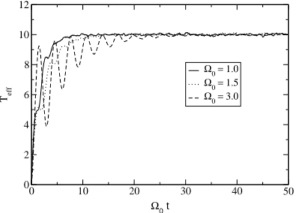
It is useful to define a time dependent effective tempera-tureTeffthrough the equipartition of the kinetic energy term,
Teff(t) =hφ˙2(t)i, where the average is over the number of
real-ization in the noise. From the equipartition theorem, at equi-librium this must correspond to the equiequi-librium temperature T. This is checked in Figs. 4 and 5, for the Markovian and non-Markovian simulations, respectively. These same figures also show that the larger isΩ0, the faster is the thermalization
of the system for the nonlocal dissipation case, in accordance to the discussed in the paragraph above.
6. CONCLUSIONS
non-502 R. L. S. Farias, R. O. Ramos, and L. A. da Silva
0 5 10 15 20 25 30
Ω0 t
-0.5 0.0 0.5 1.0
φ
Markovian
non-Markovian Ω0 = 3.0
FIG. 3: Time evolution for φ(t) in both Markovian and non-Markovian regimes andΩ0=3.0. All the other parameters are taken the same as in Fig. 1
0 10 20 30 40 50
Ω0 t 0
2 4 6 8 10 12
Teff
Ω0 = 1.0 Ω0 = 1.5 Ω0 = 3.0
FIG. 4: The effective temperature for the case of Markovian evolu-tion.
Markovian equation of motion (5) is rewritten in terms of a sixth order dynamical system (16) that is completely local in time. We have performed numerical simulations in order to compare the nonlocal dynamics with the one coming from the local approximation.
From the results of our numerical simulations, it can be seen that probably only for some very restrict region of
pa-rameters and time interval the Markovian approximation can be comparable to the non-Markovian time evolution ofφ(t). In general, we note from the results obtained that either the local approximation understimates the dissipation, or oversti-mates it in most of the region of parameters. The same can be verified varying instead ofΩ0, the parameterγof the
dis-sipation kernel [12]. The behavior of the scalar field plotted in the figures 1-4 show that the local approximation overesti-mates the dissipation of the physical system for small values ofΩ0, while for larger values ofΩ0it tends to underestimate
the dissipation at short times. This fact can, of course, con-duce to important modifications in the dynamics of models that make use of the local approximation (such as in the in-flaton dynamics during inflation). A more complete analysis
0 10 20 30 40 50
Ω0 t 0
2 4 6 8 10 12
Teff
Ω0 = 1.0 Ω0 = 1.5 Ω0 = 3.0
FIG. 5: The effective temperature for the case of non-Markovian evolution.
with more details and including multiplicative noise terms will appear elsewhere [12]. In conclusion, we have seen that for the model studied with nonlocal dissipation, the local approx-imation does not give a good representation of the dynamics.
Acknowledgments
The authors would like to thank FAPERJ, CNPq and CAPES for the financial support.
[1] L. Kofman, A. D. Linde and A. A. Starobinsky, Phys. Rev. Lett. 73, 3195 (1994).
[2] Proceedings of Quark Matter 2005, Nucl. Phys. A774, 1-968 (2006).
[3] N. C. Cassol-Seewald, R. L. S. Farias, E. S. Fraga, G. Krein, and R. O. Ramos, e-Print: arXiv:0711.1866 [hep-ph].
[4] T. Gasenzer, J. Berges, M. G. Schmidt, and M. Seco, Nucl. Phys.A785, 214 (2007).
[5] E. P. Gross, Nuovo Cim.20, 454 (1961).
[6] For a recent review, see J. Berges, AIP Conf. Proc. 739, 3 (2005).
[7] M. Gleiser and R. O. Ramos, Phys. Rev. D50, 2441 (1994). [8] A. Berera, M. Gleiser, and R. O. Ramos, Phys. Rev. D 58 ,
123508 (1998).
[9] A. Berera, I. G. Moss, and R. O. Ramos, Phys. Rev. D76 , 083520 (2007).
[10] R. L. S. Farias, PhD Thesis 2007, S˜ao Paulo State University (IFT-UNESP), S˜ao Paulo, Brasil.
[11] R. Bartussek, P. Hanggi, B. Lindner, and L. S. Geier, Physica. D109, 17 (1997).