Alexandre Cunha** Arilton Teixeira***
Summary: 1. Introduction; 2. The economy; 3. Competitive equilibrium; 4. The experiments; 5. Conclusion.
Keywords: trade blocks; tax reform; welfare.
JEL codes: D58; F11; D69.
This paper uses a general equilibrium model to evaluate the impacts of trade agreements and tax reforms on the Brazilian economy. The model predicts that welfare gains will happen whether Argentina reduces the tariffs it places on Brazilian products or the Free Trade Area of the Americas (FTAA) is implemented. However, the FTAA engenders larger welfare gains. These gains will be even larger if the FTAA is implemented simultaneously to a reduction on domestic consumption taxes. These findings suggest that most of the gains come from the reduction of Brazilian tariff and tax rates.
Adota-se neste artigo um modelo de equil´ıbrio geral para avaliar os impactos de acordos comerciais e uma reforma tribut´aria so-bre a economia brasileira. O modelo prediz que ganhos de bem-estar ocorrer˜ao se a Argentina reduzir as tarifas sobre os produtos brasileiros ou se a ´Area de Livre Com´ercio das Am´ericas (ALCA) for implementada. Contudo, a ALCA induz ganhos mais expres-sivos. Tais ganhos ser˜ao ainda maiores se a ALCA for implemen-tada simultaneamente a uma redu¸c˜ao do imposto sobre consumo. Essas conclus˜oes sugerem que a maior parte dos ganhos decorrem de redu¸c˜oes nos impostos de importa¸c˜ao e consumo existentes no Brasil.
*This paper was received in Aug. 2002 and approved in Aug. 2003. F´abio Kanzuck and an anonymous referee provided helpful comments. We thank Opencadd for providing us a Matlab license. The first author acknowledges financial support from the Brazilian Council of Science and Technology (CNPq). The usual disclaimer applies.
1.
Introduction
In the post World War II era, commerce of goods and services has increased steadily. At the same time, the world has seen the formation of trade blocks in which a group of countries agree to adopt free trade policies among themselves. Bergoeing and Kehoe (2001) provide some evidence on these facts.
A debate has surrounded the formation of each block. This debate is of particu-lar interest in a region like Latin America, where countries have generally followed what is known as import substitution policies. These policies prescribe closure of the internal market, so that domestic firms will be protected from external competition. Simultaneously, domestic producers may also receive subsidies.
In a moment when the countries of both American continents are discussing the formation of the FTAA (Free Trade Area of the Americas) the importance of studying the consequences of the formation of these blocks on the Brazilian economy speaks for itself. What are the gains from joining the FTAA? What are the consequences?
Brazilian entrepreneurs have pointed out some problems in joining the FTAA. They claim that it is difficult to compete with the US economy in a free trade zone, among other things, because of the Brazilian tax system. Brazil heavily taxes labor and also uses a cascading taxation system that increases the cost and the prices of Brazilian goods. Brazilian entrepreneurs argue that Brazil should reform its tax system before joining the FTAA.
As far as we know, this is the first study that evaluates the impacts of the FTAA and tax reform on the Brazilian economy in a unified framework. We try to assess these issues quantitatively using a computable general equilibrium model. The use of a general equilibrium model to evaluate alternative policies is today a common practice. Kehoe and Kehoe (1994b) and Kehoe and Kehoe (1994a) provide a survey on the subject.
Given the size of the US, to study the consequences of joining the FTAA is basically to study the consequences of implementing a trade agreement with the US. Therefore, we adopt a four-country (Argentina, Brazil, US and Rest of the World) model to evaluate the impacts of trade blocks and tax policies on the Brazilian economy.
the impacts of either the FTAA or tax reforms. Neither do they assess welfare gains in their simulations. The latter authors used a general equilibrium frame-work to evaluate the effects of Mercosur. They also adopt a four-country (Brazil, Argentina, Uruguay and Rest of the World) model and report welfare gains in their simulations. However, they do not consider the impacts of either the FTAA or tax reform. Therefore, we advance the research in the area by considering new questions.
We have specified our model at a very basic level. Family units are described by preference relations and budget sets. Firms are described by their production set and profit functions. The advantage of specifying the model at this structural level, instead of describing a set of demand and supply functions, is that we are able to evaluate welfare implications in an unambiguous way.
We should stress some limitations of our model. First, we are considering a static economy. In this case, we are not allowed to say anything about the transi-tion path from one steady state to another. Second, we are likely underestimating the impacts of the FTAA. As pointed out by, among others, Kim (2000) and Ty-bout and Westbrook (1995), trade liberalization is often followed by an increment in total factor productivity (TFP). Since our model is static, we cannot capture such an increment. This change in TFP would increase productivity, reduce the prices of consumption goods and increase trade and the welfare effects of the for-mation of trade blocks.
We carried out three experiments. In the first one we set the bilateral tariffs for the pair Brazil/Argentina equal to zero. We call this experiment Mercosur. The idea behind this experiment is to quantify the impacts of a reduction of the trade barriers that were raised by the Argentine government in the last few years. In the second experiment, which we call FTAA, we set all import tariffs between Argentina, Brazil and the US equal to zero. As we said before, the reason to call this experiment FTAA is that the impacts on the Brazilian economy of joining the FTAA (all American countries) should be very close to the impact of joining a free trade zone with just the US. In the last experiment, we combined the previous policy change with a reduction in Brazilian domestic taxes on consumption.
All three experiments point toward welfare gains for the Brazilian economy. These gains are very modest in the first and second. However, they are sizable in the last one (2.4% of Brazilian GDP). These results evidence a small impact of the FTAA on the Brazilian economy in the static environment used here.
is that the US has non-tariff barriers (NTBs) in many sectors, such as steel, sugar and orange juice. Additionally, the US government heavily subsidizes the country’s agricultural sector. Therefore, the effective US average tariff on Brazilian goods is higher than the one that we computed. Since we could not compute a tariff adjusted for the NTBs, we assumed that the US placed the same average tariff as the European Union on Brazilian goods. We then ran exactly the same three experiments. The impacts on the Brazilian economy were roughly the same. In particular, the welfare gains were virtually unchanged.
The computational experiments we ran suggest that most welfare gains for the Brazilian people arise from the reduction of Brazilian tariffs and domestic tax rates. This finding has a striking policy implication. Brazil should open to trade and carry out a tax reform regardless of whether or not its trade partners proceed in the same way or not.
This paper is organized as follows. In section 2 we describe the model economy. In Section 3 we define competitive equilibrium. In Section 4 we carry out the experiments. Section 5 concludes. In Section 5 (the appendix) we detail our calibration procedure.
2.
The economy
There exist four countries: Brazil (b), Argentina (a), US (u), and the Rest of the World (r). The set of countries is represented by I = {a, b, r, u}. Each coun-try produces a tradable good and a nontradable good. These goods are councoun-try specific.
Each nation i has a representative agent endowed with ¯ki units of capital and
one unit of time that she can allocate to market and non market activities (call it leisure). Capital is mobile across countries but labor is not.
Let cij denote the amount of the tradable good produced by countryiand
con-sumed in countryj; ci denotes the nontradable good of countryi. The commodity
space is L= R13. A generic point in L is denoted by x,
x = (caj, cbj, crj, cuj, ca, cb, cr, cu, la, lb, lr, lu, k)
where j ∈ I; cij is the good produced in country i and exported to country j; ci
is the nontradable good produced by country i; li is the amount of labor input in
country i and k is the capital stock.
The consumption set of a consumer in country i∈ I is
where:
li is the amount that a consumer from country i∈ I allocates to work.
ki is the amount of capital services that a consumer rents to firms, given that this
consumer has ¯ki units of capital services to be rented.
2.1
Preferences
Preferences of a consumer of country i ∈ I are represented by the utility function
ui(x) =
cαi
i
cαai
ai c αbi
bi c αri
ri c αui
ui
1−αiγ
(1−li)1−γ,
where:
αai+αbi+αri+αui = 1;cji is the good consumed by the representative consumer
in country i produced in country j;
ci is the nontradable good of country i; and
li is the amount of consumer time allocated to work.
2.2
Technologies
In each country, firms operate two technologies, one that produces the non-tradable good and one that produces the country specific non-tradable good. The production set of the nontradable good of country i∈ I is
Yi(n) =
y ∈L+ : yi ≤ kθli1−θ;yj =lj = 0 for j = i;yij = 0
,
while the production set of the tradable good of country i ∈ I is
Yi(t) =
y ∈L+ : yii ≤ kϕl1 −ϕ
i ;yij =yj = lj = 0 for j = i
.
The technological parameters satisfy θ, ϕ ∈(0,1).
2.3
Government consumption and taxes
Government ilevies proportional taxes at rateτji on the imports from country
j = i, at rate τii on the consumption of domestic goods and at rate τli on labor
income. The government uses its fiscal revenue to purchase some amount gi of its
3.
Competitive Equilibrium
A tax system for country j ∈ I is a vector τj = (τaj, τbj, τrj, τuj, τlj). An
international tax system is an object τ = (τa, τb, τr, τu). Each component of τ is a
tax system for a country. A price system for this economy is a vector
P = (pat, pbt, prt, put, pa, pb, pr, pu,−wa,−wb,−wr,−wu,−r).
We are abusing notation, since prices of nontradable goods from other countries are infinity. But this abuse make our notation easier and homogeneous across countries. The coordinates of P are before-tax prices. An after-tax price system for a country i is a vector
Pi = (pai, pbi, pri, pui, pan, pbn, prn, pun,−pal,−pbl,−pul,−prl,−r)
The typical consumer from county i ∈ I solves the following problem
max
x∈Xi
u(x) s.t. Pi·x ≤0
The problem of a firm that produces the nontradable good in country i∈ I is
max
y∈Yi(n)
P ·y
The problem of a firm that produces the tradable good in country i∈ I is
max
y∈Yi(t)
P ·y
Definition 3.1 A competitive equilibrium for an international tax system τ is an
array P,(Pi, xi, yin, yit)i∈I
such that:
1. given P, yin and yit solve the problem of the respective firm;
2. given Pi, xi solves the maximization problem of consumer i;
3. P, Pi and τi satisfy (1 +τai)pat = pai, (1 +τbi)pbt = pbi, (1 +τri)prt = pri,
(1 +τui)put =pui, (1 +τii)pi = pin, and (1−τli)wi =pil.
4. each government balances its budget, that is,
pjgj = τljwjlj +
i∈I
5. (xi, yin, yit)i∈I is feasible, that is,
ci+gi = kθinl1 −θ in ,
j∈I
cij = kitϕl 1−ϕ
it ,
lin +lit =li ,
i∈I
(kin +kit) =
i∈I
¯ ki .
One may wonder why a balance-of-payment constraint was not considered in the above definition. It can be shown that the conditions spelled out in definition 3.1 imply that each country satisfies its balance-of-payment constraint.
4.
The Experiments
The goal of this section is to evaluate welfare consequences and real effects of trade agreements and a tax reform for the Brazilian economy. To carry out this task, we proceeded in the following way. First, we calibrated the model so that it matched some selected features of the actual Brazilian, US, Argentinian and world economies. The calibration procedure is explained in detail in the appendix. Then, we computed the competitive equilibrium associated with the calibrated param-eters. This equilibrium is our benchmark. Finally, we computed the competitive equilibria for three distinct international tax systems and compared the outcomes. The calibrated tariff and tax rates for Brazil, Argentina and the USA are given below:
Table 1
Calibrated tariffs and tax rates - % values
Country Argentina Brazil Rest of the World USA Labor Income Tax
Argentina 21 9.3 18.4 18.4 23.61
Brazil 0 16.2 23 23 18
US 1.94 2.52 2.01 5.467 27.733
Each line indicates how a country taxes its domestic goods and the goods produced by other countries, as well as its tax on labor income.
In the first experiment we simply droppedτba from its original value (i.e., 9.3%)
to 0. Observe that in this model economy a complete implementation of Mercosur amounts to setting both τab and τba equal to zero. Since the original (i.e., the
In the second experiment we set τba = τua = τab = τub = τau = τub = 0. This
amounts to setting all intra-American trade tariffs in the model equal to zero. Therefore, we denominated this experiment FTAA.
The third experiment combines the FTAA with a reduction of the consumption taxes in Brazil. We lowered τbb from its original value of 16.2% to 5.467% (the
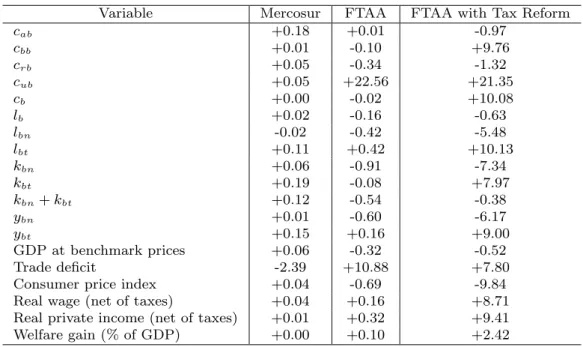
level observed in the United States). We called this experiment FTAA with tax reform. The main results are presented in table 2.
We measured the welfare gain using equivalent variation as a percent of bench-mark GDP. All other figures in the table are percent changes from the benchbench-mark competitive equilibrium.
The equivalent variation is a standard measure of welfare gains and/or losses in general equilibrium analysis. Let Pb0 be the price vector faced by the Brazilian consumer and u0 the utility level she obtained before the reform. Let u1denote the post-reform utility level andE(Pb, u) the expenditure function. The equivalent
variation is given by E(Pb0, u1)−E(Pb0, u0). Observe that this difference tells how much extra income the consumer would need, at benchmark prices, to obtain the post-reform utility. For more on the equivalent variation and other welfare measures, see Varian (1992).
In the Mercosur experiment, the Brazilian trade deficit fell 2.39%. All other variables changed by less than 0.2%. The welfare gains for the Brazilian people were very modest. A factor behind the small impact of a drop inτbain the Brazilian
economy is the relative size of the countries. The Brazilian GDP is almost three times Argentina’s GDP. Kehoe and Kehoe (1994a) stated that “because Mexico’s economy is the smallest, it will enjoy the biggest NAFTA-produced increase in economic welfare” and “NAFTA’s impact on the United States, although positive, is barely perceptible as a percentage of GDP.” So, our finding is perfectly consistent with earlier studies.
Despite the small impact of the fall inτba on the Brazilian economy, the
Merco-sur experiment provides some insights. Since both kbn and kbt went up, Mercosur
Table 2 Experiments’ results
Variable Mercosur FTAA FTAA with Tax Reform
cab +0.18 +0.01 -0.97
cbb +0.01 -0.10 +9.76
crb +0.05 -0.34 -1.32
cub +0.05 +22.56 +21.35
cb +0.00 -0.02 +10.08
lb +0.02 -0.16 -0.63
lbn -0.02 -0.42 -5.48
lbt +0.11 +0.42 +10.13
kbn +0.06 -0.91 -7.34
kbt +0.19 -0.08 +7.97
kbn+kbt +0.12 -0.54 -0.38
ybn +0.01 -0.60 -6.17
ybt +0.15 +0.16 +9.00
GDP at benchmark prices +0.06 -0.32 -0.52
Trade deficit -2.39 +10.88 +7.80
Consumer price index +0.04 -0.69 -9.84
Real wage (net of taxes) +0.04 +0.16 +8.71
Real private income (net of taxes) +0.01 +0.32 +9.41
Welfare gain (% of GDP) +0.00 +0.10 +2.42
The FTAA experiment generated an increase of 10.88% in the Brazilian trade deficit. The welfare gain was 0.10% of the benchmark GDP. This is still a modest figure, but far larger than the Mercosur one. Brazilian consumption of the Amer-ican tradable good (cub) increases by 22.56%. All other variables changed by less
than 1%. So, except for the trade balance and cub, the FTAA has small impacts
on the variables.
Observe that both cab and cub went up, while lb, cb, cbb and crb fell. There was
a reallocation of labor from the nontradable to the tradable sector of the Brazilian economy. Capital utilization went down in both sectors. So, a capital outflow took place. The tradable output went up, while the nontradable one went down. Both GDP and CPI went down. Real wages and real private income experienced an increase.
We do not report these data here, but it is worth mentioning that the FTAA has negligible effects on the rest of the world. Particularly, krn and krt are roughly
The Mercosur experiment showed that when a trade tariffτij is reduced, capital
flows from country j to country i. In the FTAA experiment, several τij’s were
simultaneously reduced. Thus, it is not possible to anticipate which country should receive or send capital abroad. It turned out that United States received capital, while Brazil and Argentina lost it.
This result about capital deserves more attention. Evidence from the formation of European Union indicates that the capital movement goes from the richest countries to the poorest ones. So, if the same were to happen with the FTAA, Brazil should benefit from a capital inflow.
Kehoe and Kehoe (1994b) discuss in detail the issue of capital flows in models of trade agreements. They show that larger welfare gains take place when there is a capital flow. However, any static model will hardly generate a capital flow from a richer to a poorer country. What drives capital movement is the capital rate of return. Hence, a possible way that a model can generate a capital flow to a poorer country is by means of a productivity increase.
Kim (2000) provides evidence that trade liberalization had a positive impact on the productivity of Korean manufactures. Tybout and Westbrook (1995) shows that a similar event took place in Mexico during the trade liberalization of the 90s. Herrendorf and Teixeira (2001), Holmes and Schmitz (2001) and Holmes and Schmitz (1995) show, from a theoretical point of view, that trade liberalization may have a positive impact on a country’s productivity.
Despite not capturing the productivity surge and capital flow associated with trade opening, the model still predicts welfare gains in both the Mercosur and FTAA experiments. We believe that these gains are lower bounds. We anticipate that a more sophisticated model will display even larger welfare improvements.
The observed GDP fall in the FTAA experiment also deserves attention. That fall was driven by a drop in ybn. Observe that when the Brazilian government
reduces tariffs and tax rates, there is a fall in government fiscal revenue. This will lead to a decrease in gb and a consequent fall in ybn.
The aforementioned fall in gb brings an important point to light. A reduction
of the tax burden, as was done in the above experiments, has to be accompanied by a reduction in government expenditures. An interesting exercise would consist of opening the Brazilian economy to international trade and raising some tax rates to compensate for the tariff reduction. This exercise is left for future research.
The FTAA with tax reform experiment generated a huge welfare gain (when compared to the previous two). There was a gain on the order of 2.42% of GDP. The Brazilian consumer substituted away from cab and crb toward cbb, cub, cb and
Recall that our model is static. Thus, statements about capital flows have to be evaluated with care. Anyway, it is interesting to see that in the FTAA experiment the sum kbn+kbt went down by 0.54%, while in the last experiment
it went down by a smaller amount (0.38%). Hence, the third experiment suggests that a tax reform may help Brazil to attract capital.
The third experiment generated a flow of production factors to the tradable sector. Both lbt and kbt went up. Resources left the nontradable sector. As a
consequence of this reallocation of resources, ybt grew and ybn fell.
The aforementioned fall in GDP was larger than in the FTAA experiment. Again, this fall was driven by the reduction in gb. The trade deficit increased, but
less than in the FTAA simulation. On the other hand, the decrease in the CPI and the increase in net real wages and net private income were by far larger.
Let us analyze the last experiment carried out in this paper. The calibrated value of τbu was 2.52%. As mentioned in the appendix, this number is a weighted
average of tax rates on Brazilian exports to the US. This procedure does not take into consideration non-tariff barriers, as quotas. So, the effective tariff rate is clearly higher than 2.52%. To address this issue, we proceeded as following: we assumed that τbu was equal to 8.1% (which is the average tariff that the
Euro-pean Union places on Brazilian products) and ran the three experiments again. Surprisingly, the results did not change much. We report them in table 3. In the particular case of welfare gains, the differences are negligible.
This finding has a striking policy implication. The model suggests that most of the gains Brazil can obtain from a trade agreement come from the reduction of Brazilian tariffs. More specifically, a unilateral reduction of Brazilian tariffs would increase welfare. Besides, if this unilateral reduction of tariffs were also followed by a tax reform, the welfare gains would be substantial.
The conclusion that a reduction in domestic taxation induces larger welfare gains has an intuitive explanation. Consider the tariffs imposed by the US on the goods imported from Brazil. Even when we increased this average tariff from 2.52% to 8.1% this tariff is still small when compared to the taxation that Brazil imposed on consumption of the domestic good. That is, the distortions that the US government places are too small compared to the distortion introduced domestically. Therefore, substantial welfare gains can be obtained by a unilateral reduction of Brazilian taxes and tariffs.
Table 3
Experiments’ results for a higher initial US tariff on brazilian goods
Variable Mercosur FTAA FTAA with Tax Reform
cab +0.18 +0.07 -0.91
cbb +0.01 -0.08 +9.77
crb +0.05 -0.28 -1.27
cub +0.05 +22.63 +21.42
cb +0.00 -0.02 +10.09
lb +0.02 -0.13 -0.61
lbn -0.02 -0.44 -5.50
lbt +0.11 +0.55 +10.26
kbn +0.06 -0.85 -7.27
kbt +0.19 +0.13 +8.20
kbn+kbt +0.12 -0.40 -1.10
ybn +0.01 -0.59 -6.16
ybt +0.15 +0.33 +9.18
GDP at benchmar prices +0.06 -0.25 -0.45
Trade deficit -2.33 +8.00 +5.00
Consumer price index +0.04 -0.64 -9.79
Real wage (net of taxes) +0.04 +0.20 +8.75
Real private income (net of taxes) +0.01 +0.34 +9.43
Welfare gain (% of GDP) +0.00 +0.10 +2.42
5.
Conclusion
A small-scale general equilibrium model was used to evaluate the impact of trade agreements and tax reforms on the Brazilian economy. The main finding is that most of the welfare gains arise from reduction of Brazilian domestic taxes and import tariffs. A reduction of trade tariffs charged by foreigners on Brazilian goods does not have large welfare effects on Brazilian individuals.
The tariff and tax reductions performed in this paper were not compensated by an alternative source of revenue for the government. Consequently, the real government expenditure was reduced in most of the experiments. An interesting exercise would consist of carrying out a tariff reduction compensated by a tax increase in another sector of the economy so that government revenue would remain constant.
References
Bergoeing, R. & Kehoe, T. (2001). Trade theory and trade facts. Federal Reserve Bank of Minneapolis Research Department, Staff Report 284.
Bugarin, M., Ellery Jr., R., Gomes, V., & Teixeira, A. (2002). The Brazilian depression in the 1980s and 1990s. Unpublished manuscript, 2002.
Bulacio, J. (1999). La carga impositiva sobre el capital e el trabajo. Anales de la XXXIV Reuni´on de La Asociaci´on Argentina de Econom´ıa Pol´ıtica.
Castilho, M. (2001). O acesso das exporta¸c˜oes do Mercosul ao mercado europeu. Anais do XXIX Encontro Nacional da Associa¸c˜ao Nacional dos Centros de P´ os-Gradua¸c˜ao em Economia.
Cavalcante, J. & Mercenier, J. (1999). Uma avalia¸c˜ao dos ganhos dinˆamicos do Mercosul usando equil´ıbrio geral. Pesquisa e Planejamento Econˆomico, 29(2):153–184.
Cooley, T. & Prescott, E. (1995). Economic growth and business cycles. In Cooley, T. E., editor, Frontiers of Business Cycle Research. Princeton University Press, Princeton.
Gonzaga, G., Terra, M. C., & Cavalcante, J. (1998). O impacto do Mercosul sobre o emprego setorial no Brasil. Pesquisa e Planejamento Econˆomico, 28(3):475– 508.
Herrendorf, B. & Teixeira, A. (2001). How trade policy affects technology adoption and total factor productivity. Unpublished manuscript.
Holmes, T. & Schmitz, J. (1995). Resistance to new technology and trade between areas. Federal Reserve Bank of Minneapolis Quarterly Review, 19(1):2–17.
Holmes, T. & Schmitz, J. (2001). A gain from trade: From unproductive to productive entrepreneurship. Journal of Monetary Economics, 47(2):417–446.
IMF (2001). Direction of Trade Statistics Yearbook. IMF, Washington.
Kehoe, P. & Kehoe, T. (1994b). A primer on static applied general equilibrium models. Federal Reserve Bank of Minneapolis Quarterly Review, 18(2):2–16.
Kim, E. (2000). Trade liberalization and productivity growth in Korean manufac-ture industries: Price protection, market power and scale efficiency. Journal of Development Economics, 62(1):55–83.
Kydland, F. & Prescott, E. (1982). Time to build and aggregate fluctuations. Econometrica, 50(6):1345–1370.
Lejour, A., Mooji, R., & Nahuis, R. (2001). EU enlargement: Economic impli-cations for countries and industries. CPB Netherlands Bureau for Economic Policy Analysis, document 11.
Mendoza, E., Razin, A., & Tesar, L. (1994). Effective tax rates in macroeconomics: Cross-country estimates of tax rates on factor incomes and consumption. Jour-nal of Monetary Economics, 34(3):297–323.
Rebelo, S. (1997). What happens when countries peg their exchange rates? Na-tional Bureau of Economic Research, working paper 6168.
Rebelo, S. & V´egh, C. (1995). Real effects of exchange rate based stabilization: An analysis of competing theories. National Bureau of Economic Research, working paper 5197.
Rosal, J. M. & Ferreira, P. (1998). Imposto inflacion´ario e op¸c˜oes de financiamento do setor p´ublico em um modelo de ciclos reais de neg´ocios para o Brasil. Revista Brasileira de Economia, 52(1):3–37.
Siqueira, R., Nogueira, J. R., & Souza, E. (2001). A incidˆencia final dos impostos indiretos no Brasil: Efeitos da tributa¸c˜ao de insumos. Revista Brasileira de Economia, 55(4):513–544.
Tybout, J. & Westbrook, M. D. (1995). Trade liberalization and the dimensions of efficiency change in Mexican manufacturing industries. Journal of International Economics, 39(1-2):53–78.
Varian, H. (1992). Microeconomic Analysis. W. W. Norton & Company, New York.
Appendix
The following list of parameters have to be calibrated: αj, αaj, αbj, αrj, αuj,
γ, ¯kj, θ, ϕ, τaj, τbj, τrj, τuj, τlj. We calibrated the model to match some features
of the US, Brazil, Argentina and the Rest of the World economies in 1997. Our procedure is detailed below.
Following Kydland and Prescott (1982), we set γ = 2/3. We borrow from Rebelo (1997) and Rebelo and V´egh (1995) the shares θ = 0.37 and ϕ= 0.52.
To calibrate the trade tariffs we proceeded as follows.
1. US:
We used the data provided by the US International Trade Commission to calculate the weighted average tariff imposed on Brazilian, Argentine and an Rest of the World goods. Weights were by given the participation of each good in the total trade with the respective country. The values we obtained are τau = 1.94%, τbu = 2.52% and τru = 2.01%.
2. Brazil and Argentina:
We took the simple average of Mercosur tariff information provided in Gon-zaga, Terra and Cavalcante (1998). The values we obtained are τba = 9.3%,
τra =τua = 18.4%, τab = 0 and τrb = τub = 23%.
3. Rest of the world:
We took the simple average of the European Union tariffs provided in Lejour et al. (2001) to setτur = 4.32%. We picked a weighted average tariff provided
by Castilho (2001) to set τar = τbr = 8.1%.
To calibrate the tax rates on labor income and domestic consumption, we took the steps detailed below.
1. US:
Mendoza et al. (1994) estimated tax rates on labor income and consumption for several OECD countries. In an updated version of their work (which is available at www.econ.duke.edu/˜mendonzae), they provided estimates for these variables for 1996. We used their figures to set τlu = 5.467% and
2. Brazil:
We used the calibration carried out by Rosal and Ferreira (1998) to set τlb = 18%. The paper on tax incidence of Siqueira et al. (2001) led us to set
τbb = 16.2%.
3. Argentina:
Bulacio (1999) estimatedτla = 23.61% and Zee (1998) estimated τaa = 21%.
4. Rest of the world:
The updated version of Mendoza et al. (1994) provides average labor income and average consumption tax figures for Canada, France, Germany, Italy, Japan, and the United Kingdom. Using PPP GDP as weights, we took the weighted average of these countries taxes and obtained τlr = 36.39%
and τrr = 9.31%. Note that these countries amount to 75% of the world’s
(excluding US, Brazil and Argentina) PPP GDP.
To calibrate the αj’s and αij’s we proceeded as follows.
1. αj:
For Brazil, the US and Argentina, we set αj equal to the ratio of each
country’s service output to its GDP. This data is provided by the World Bank (1999) . This procedure yielded αa = 63%, αb = 50% and αu = 72%.
To calibrate αr we used the formula
αr =
αwYw −αaYa−αbYb −αuYu
Yw −Ya−Yb−Yu
= 0.5992,
whereYw is the world’s GDP andαw the world’s services output as a fraction
of Yw (both αw and Yw are provided in the aforementioned publication and
Yj is country j’s GDP). To round off, we picked αr = 60%.
2. αaj, αbj, αrj, αuj:
To explain how we calibrated these parameters, we will take Argentina as our example. The same procedure was used for Brazil and the US. From the Argentine consumer first order conditions we have
(1−αa)αja
αa
= (1 +τja)pjtcja (1 +τaa)paca
In the above expression, pjtcja is the value of Argentina’s imports from
country j and paca is equal αaYa (see the above section). We computed
prtcra as a residue. That is, let Ma be the value of total Argentine imports.
Therefore,prtcra = Ma−pbtcba−putcua. The IMF (2001) provides the figures
for Ma, pbtcba and putcua. We obtained αba ∼= 0.0516, αra ∼= 0.1425 and
αua ∼= 0.0497. Sinceαaa+αba+αra+αua = 1, thenαaa ∼= 0.7561. By taking
the same steps for Brazil and the US, we got αab ∼= 0.0178, αbb ∼= 0.8374,
αrb ∼= 0.1063, αub ∼= 0.0386, αau = 0∼ .0011, αbu ∼= 0.0045, αru ∼= 0.3952,
and αuu ∼= 0.5992. To obtain αar, αbr, αrr, and αur, an additional step was
required. By taking the total Brazilian, Argentine and American exports and subtracting the value each of them exported to the other two we computed the amount each of these countries exported to the Rest of the World, as well as the total imports of the Rest of the World. With this information at hand, we applied the procedure detailed above. This led to αar ∼= 0.0020,
αbr ∼= 0.0048, αrr = 0∼ .9109, and αur ∼= 0.0823. The values here use the
“∼=” sign because they were in reality computed to more than four decimal places.
To calibrate the ¯kj’s we proceed as follows.
1. US:
According the World Bank (1999), the US GDP was equal to US$ 7.745705 trillion in 1997. Cooley and Prescott (1995) estimated that US’s capi-tal/output ratio is close to 3.32. We use these information to set ¯ku =
3.32×7.745705×1012.
2. Brazil and Argentina:
Using the data on GDP and GNP in current dollars and PPP GNP dol-lars provided by the World Bank (1999), one can estimate the PPP GDP for both Brazil and Argentina. We obtained YP P P
a ∼= 374,776.415 million
and YP P P
b ∼= 1,037,130.429 million. Bugarin et al. (2002) estimated a
capi-tal/output ratio of 2.3 for the Brazilian economy. We then set ¯kj = 2.3YjP P P
for j =a and j = b.
3. Rest of the World:
We used the procedure mentioned in the previous item to find thatY P P P
r ∼=