Ribosome binding site recognition using neural networks
Márcio Ferreira da Silva Oliveira
1, Daniele Quintella Mendes
2, Luciana Itida Ferrari
1and Ana Tereza Ribeiro Vasconcelos
11
Laboratório Nacional de Computação Científica, Coordenação de Matemática Aplicada,
Laboratório de Bioinformática, Petrópolis, RJ, Brazil.
2
Universidade Federal do Rio de Janeiro, Coordenação de Pós-graduação e Pesquisa de Engenharia,
Programa de Engenharia de Sistemas e Computação, Rio de Janeiro, RJ, Brazil.
Abstract
Pattern recognition is an important process for gene localization in genomes. The ribosome binding sites are signals that can help in the identification of a gene. It is difficult to find these signals in the genome through conventional methods because they are highly degenerated. Artificial Neural Networks is the approach used in this work to address this problem.
Key words:bioinformatics, neural networks, ribosome binding site.
Received: August 15, 2003; Accepted: August 20, 2004.
Introduction
Pattern recognition is an important process for local-ization of functional sequences in genomes, such as genes, promoters, or regulators (for example,SOS boxes1andLux boxes2). For many reasons, it is difficult to find some of
these patterns in a genome, but generally this is because there is a great variation in the composition or localization of these sequences, or because there is not enough knowl-edge about them. Pattern recognition methods can be used to overcome these problems. TheRibosome Binding Site (RBS)is one of those important signals for the
identifica-tion of genes in a DNA sequence, since almost every bacte-rial mRNA (messenger RNA) has an RBS, to the polypeptidical product to be produced.
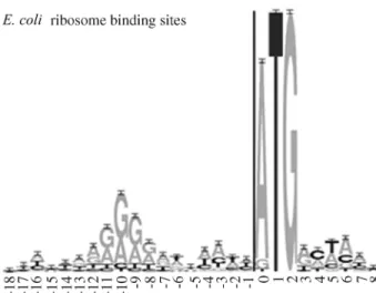
The RBS is the region where the ribosome binds to an mRNA to begin the translation of the mRNA into a protein. In the literature it is possible to find a large variety of defini-tions for RBS, but some characteristics can be pointed out
(Shultzbergeret al., 2001; Alberts, 1994) (Lodish, 2000;
Lewin, 1999). These are shown in Figure 1.
• RBS sequences are rich in purine bases,i.e., rich in Adenine (A) and Guanine (G);
• They are localized from three to 14 base pairs up-stream from the beginning of a gene3;
• Their size vary from three to nine base pairs; • Their consensus sequence is “A G G A G”; • The RBS sequences are complementary4to the
py-rimidine-rich sequence found in the rRNA in the 16S unit of the ribosome (end 3’ - HO-A U U C C U C C A C U A G -5’).
The RBS sequence is highly degenerated, and may have a great variation in its base composition and localiza-tion in the genome, as shown in Figure 2. Due to this great flexibility, the conventional methods generally used to rec-ognize RBS’s might have a very high error rate in their pre-dictions.
In this work, a Machine Learning approach (Mitchell, 1997; Carvalho, 2001) was used, due to its capability of dealing with this kind of problem, where there is little infor-mation or highly imprecise data to be analyzed.
www.sbg.org.br
Send correspondence to Ana Tereza Ribeiro Vasconcelos. Labora-tório Nacional de Computação Científica, Coordenação de Mate-mática Aplicada, Laboratório de BioinforMate-mática, Av. Getulio Vargas 333, Quitandinha, 25651-075 Petrópolis, RJ, Brazil. E-mail: [email protected].
Research Article
1 These are sequences that may indicate that a gene belongs to theSOS Regulation System, that is activated when there is a damage to
the DNA.
2 These are sequences that may indicate that a gene belongs to theQuorum Sensing System, which is responsible for “counting” the number of individuals of the same species.
3 In the beginning of a gene usually there is a sequence of adenine-thymine-guanine bases (ATG), known as astart codon.
More specifically, a Multi-Layer Neural Network (MLNN), with the Backpropagation learning algorithm (Haykin, 1998 Wu, 2000), were employed. The MLNN was chosen because the knowledge can be taught to the net-work through exposure to examples, in a learning process. In this work, the concept of the RBS will be learned from a set of nucleic bases sequences that represent the problem adequately; this will be shown in the next section. Indeed, the Backpropagation algorithm figures among the simplest ones in the Artificial Neural Network universe. Because of this, it was chosen for an initial work in this issue.
As a special contribution, this work emphasizes the need for the creation of biological data mining tools capa-ble of capturing both imprecision and ambiguity present in biological data.
Material and Methods
We carried out this work through successive steps, in order to construct a neural network capable of learning the RBS concept, quite independently from the enormous data quantity generated by genome sequencing. For each step, a
different model was designed for both architecture and data codification.
Three models of MLNN were built and, for each one, tests were performed with several different parameters, such as training strategy, learning step, and maximum error rate. For each of the models the best results are shown, and one network from each model is indicated as having the best performance. This performance is calculated using these values:
•True Positive(TP): percentage of instances that the
network correctly classified a RBS sequence;
•True Negative(TN): percentage of instances that the
network correctly classified as not being a RBS sequence; •False Positive(FP): percentage of instances that are
not RBS sequences, but the network classified as a RBS se-quence;
•False Negative(FN): percentage of instances that
are RBS sequences, but the network classified as not being a RBS sequence.
First model
The training of the first model was done using exam-ples of sequences, which were taken from a well-known software for RBS identification: the RBSFinder (Suzek, 2001), whose default output is five bases length sequences. Therefore, this will be the size of the input of the networks of this model.
The codification used in this work is a normalized Bi-nary Four Digit One (known as BIN4) (see Table 1), which in Wu (2000) is the most recommended for Bioinformatics applications.
The networks were built with 20 units in the input layer. The number of neurons in the hidden layer, the learn-ing step, and the maximum error rate were empirically de-termined.
To assemble the output layer, it is interesting to know how the sequences are presented in the decision space formed by the network. The codification also has an influ-ence on the determination of the number of units in the out-put layer. For evaluating the effects of the codification over the network’s decision space, we used a clustering algo-rithm, known as an “Elastic Algorithm” (Salvini, 2000).
We have presented the codified sequences to the Elas-tic Algorithm, which answered with four sequence clusters. The fact that the Elastic Algorithm separated these se-quences into different clusters does not necessarily mean that there are different kinds of RBS. It just suggests that the codification chosen separates the sequences in four Figure 1- Sequence Logo built using 149 selected sequences of theE. coli
genome. The RBS pattern can be seen between the positions -13 and -6, where there is a high concentration of purine bases. Figure taken from Schneider (1990).
Figure 2- Selected parts of theE. coligenome. The RBS sequences are underlined, and the names of the genes they correspond to are on the left. Adapted Figure from Alberts (1994) page 401.
Table 1- Nucleic bases codification.
0.9 0.1 0.1 0.1 Adenine
0.1 0.9 0.1 0.1 Thymine
0.1 0.1 0.9 0.1 Guanine
clusters, indicating that there are four patterns to be recog-nized. So, the output layer was built with four units, one for each cluster. Each of these units has an output value of be-tween 0.1 and 0.9. The highest output value among the four units indicates which cluster the sequence belongs to, and this value has to be greater than a 0.5 threshold. If the four units answer values are lower than this threshold, it is con-sidered a negative answer,i.e., the tested sequence is not
part of any RBS cluster.
From the 49 sequences presented to the Elastic Algo-rithm, 10 were chosen to constitute the training set, because these are more representative of the four clusters. These se-quences are the positive examples. The negative examples of the training set were built by making the complement of the positive set. For example, a positive sequence A G G A G will generate the sequence T C C T C as a negative exam-ple.
From those sequences that were not chosen to be the positive examples of the training set, 12 were chosen for the test set. Their complements were built to be the negative ex-amples of the training set.
As we will argue in more detail in the Discussion, both training and test sets had to be structured under some restrictions. The number of examples available were rather limited and we decided, with this model, to keep the RBSFinder data format in order to make comparisons as re-liable as possible with well recognized software which ad-dresses the same issue.
The results of the three best networks for this model can be seen in Table 2. The best performance for the first model was the 20-4-4-architecture network.
Second model
In this model we used the same codification as pre-sented in the first one, so there were no changes in the input layer. But as a different training strategy was implemented, the hidden and output layers, as well as the learning step and the maximum error rate were altered.
As stated above, RBS sequences have a high concen-tration of purine bases (A and G), which can be easily seen in the output of the RBSFinder in its analysis over theE. coli genome. Based on this information, we decided to
model this concept explicitly, through the sequences used to train the network. So, the training set was built with only four sequences: A A A A A and G G G G G, representing the purines as positive examples; and C C C C C and T T T T T, representing the pyrimidines as negative examples.
This approach for addressing a pattern recognition problem is quite different from what it is currently found in Artificial Neural Network applications. Indeed, it was our aim to develop a way of representing a RBS concept as sim-ply as possible, based upon its biological characteristics.
One observation concerns the negative examples: these were represented by the complement of the positive ones because in most of the cases they indeed are their com-plement. The results showed that this strategy can be a good choice.
Only one unit, with answer values varying between 0.1 to 0.9 , was chosen to compose the output layer. Output values close to 0.1 are considered negative answers, and those close to 0.9 are considered positive answers, with a 0.5 threshold. The other parameters were chosen empiri-cally, as in the previous model.
In this model we used the same test set of the first model to evaluate the performance. The best architectures for this model can be seen in Table 3, and the one indicated as having the best performance is the 20-2-1.
Third model
In the third model, the codification was modified to address the concept that RBS are sequences rich in purine bases using a different strategy. Table 4 shows the codifica-tion used.
This codification does not distinguish bases of a same family; instead it groups them in purines (A and G) and py-rimidines (C and T). The training set is the same as the one
Table 2- Comparison between the first model networks. The column Architecture(x-y-z) indicates the number of units in the input, hidden, and output
layers, respectively. The column MC (Misclassified) indicates that the network correctly classified a sequence as a RBS, but in the wrong cluster.
Architecture (x-y-z) Learning step Max. error rate TP(%) TN(%) FP(%) FN(%) MC(%)
20-2-4 0.3 0.001 33.4 16.6 33.4 00.0 16.6
20-3-4 0.1 0.01 33.4 33.4 16.6 4.1 12.5
20-4-4 0.2 0.001 37.5 41.7 8.3 00.0 12.5
Table 3- Comparison between the second model networks. The column Architecture(x-y-z) indicates the number of units in the input, hidden, and output layers, respectively.
Architecture (x-y-z) Learning step Max. error rate TP(%) TN(%) FP(%) FN(%)
20-1-1 0.2 0.001 45.9 50.0 00.0 4.1
20-2-1 0.1 0.01 50.0 50.0 00.0 00.0
used in the second model, reinforcing the concept of purine rich sequences.
As the codification size is now one digit for each base (instead of the four digits used in the previous models), the quantity of units in the input layer was reduced to five, one for each base of the sequences that will be presented to this layer.
As in the second model, there is only one unit in the output layer to classify a sequence as positive or negative. The threshold remains 0.5.
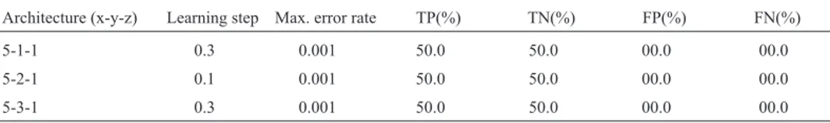
The number of units in the hidden layer, the learning step and the maximum error rate were chosen empirically, as in the previous models. In this model we used the same test set of the previous models to evaluate the performance, and the outcome can be seen in Table 5.
The same questions involving training and test sets, as was mentioned for the second model in the previous subsection, will be examined more in depth in the Discus-sion.
Model validation
As mentioned before, the neural networks were trained with variations in parameters, such as learning and error rates. The condition for learning interruption was based on the error rate. The values of learning parameters presented by the best neural networks may be observed in Tables 2, 3 and 5. Therefore, each neural network presented a particular performance measured by its numbers of right and wrong answers, when applied over the test set.
Observing the recognition ability of the three archi-tectures, the one indicated as having the best performance was the 5-2-1-architecture network, for this one had its an-swer values closer to the goal values (i.e., positive answers
closer to 0.9, and negative answers closer to 0.1).
The neural networks which obtained the best perfor-mances were chosen for later refinement. The best one for each strategy, after refinement, was employed for compari-sons between the three models and for validation withE.
coli data extracted from Regulon DB (Colado-Vides,
1998).
Here, two additional test phases will be shown: first, the networks were validated using sequences previously experimentally tested; later, the networks were tested over the entireE. coligenome. For these two test phases, only
the networks chosen in each model as having the best per-formance were used.
In order to read and present the nucleic sequences to the MLNN, we used asliding window. This window
con-sists of an array of nucleic bases that will be read at once (from the experimental data, or from theE. coligenome),
codified, and then presented to the MLNN’s input layer. Then, this window slides to the next base, and this new se-quence is read and codified until this window slides through the entire selected area.
The Escherichia coli K-12 MG1655 genome
(U00096) was used to evaluate and compare the three mod-els. To validate the models, we used a database containing 137 sequences that were experimentally tested from theE. coligenome, taken from the Regulon DB (Collado-Vides,
1998). The sequences are 30 bases length, as displayed in Figure 3.
For estimating the number of true positives and false negatives, we created a set of positive sequences, using the 10 bases from region “a” in Figure 3 of the 137 Regulon DB sequences. In order to obtain just one answer for each gene, only the highest output of the networks was considered for each start codon coordinate.
For the set of negative sequences construction, in or-der to calculate the true negative and false positive cases, 1470 sequences were extracted from the 20 bases of the re-gions “b” as in Figure 3.
Results
We analyzed several different thresholds for each net-work, until we obtained the values shown in Tables 6, 7 and 8. The threshold tests began with the value 0.5, as this Table 4- Nucleic base codification.
0.9 Adenine
0.1 Thymine
0.9 Guanine
0.1 Cytosine
Table 5- Comparison between the second model networks. The column Architecture (x-y-z) indicates the number of units in the input, hidden, and output
layers, respectively.
Architecture (x-y-z) Learning step Max. error rate TP(%) TN(%) FP(%) FN(%)
5-1-1 0.3 0.001 50.0 50.0 00.0 00.0
5-2-1 0.1 0.001 50.0 50.0 00.0 00.0
5-3-1 0.3 0.001 50.0 50.0 00.0 00.0
threshold was used in all the models previously described. The tests were done from this value to 0.8, with a 0.1 step, and from the data obtained it was possible to see that the best outcomes were between 0.7 and 0.8. So, additional tests were done, starting with 0.7, using a 0.01 step.
Due to the highly degenerated characteristic of the RBS sequences, the MLNN were trained to allow general-ization at high levels, increasing the maximum error rate accepted. It causes a reduction in the difference between the values of positive and negative answers, as can be seen in the comparison of the behavior of the models with different threshold values.
We chose a best threshold for each network analyzing the data in the Tables 6, 7 and 8. This choice was con-strained by the fact that we want to reduce the false positive quantity, without increasing the false negative quantity. The best thresholds for each model are: 0.72 for the first model; 0.71 for the second model; and 0.74 for the third model.
Recognition of ribosome binding sites inE. coli The graph in Figure 4 shows the answer values for the three models, for each sequence position analyzed up-stream from the start codon. In the graph in Figure 4, it is
possible observing that the networks of the second and third models presented higher answer values in the RBS region. On the other hand, the first model network presented higher answer values in many positions. The graph shows a posi-tive outcome, for the networks identified RBS sequences within the expected localization, though they were not trained explicitly with information about the position up-stream from the start codon.
In the individual evaluation of answers of networks for each start codon, it was noted that there was a high level of generalization, identifying many possible RBS se-quences for a single gene. It was a predicted result due to the training strategies chosen. In Figure 5 it is possible to observe that, in some cases, the answer values increase as the window slides towards the start codon, up to a certain point. From this point on, the answer values begin to de-crease. This might be due to the variation of the RBS’s size, and because the network was not trained explicitly with in-Table 6- Performance evaluation for model 1.
Threshold
0.71 0.72 0.73
Positive instances:
TP (%) 99.27 99.27 98.54
FN (%) 0.73 0.73% 1.46
Negative instances:
TN (%) 79.25 80.00 82.11
FP (%) 20.75 20.00 17.89
Table 7- Performance evaluation for model 2.
Threshold
0.70 0.71 0.72
Positive instances:
TP (%) 99.27 99.27 98.54
FN (%) 0.73 0.73 1.46
Negative instances:
TN (%) 78.37 80.27 81.97
FP (%) 21.63 19.73 18.03
Table 8- Performance evaluation for model 3.
Threshold
0.73 0.74 0.75
Positive instances:
TP (%) 100.00 100.00 98.54
FN (%) 0.00 0.00 1.46
Negative instances:
TN (%) 68.91 72.79 80.00
FP (%) 31.09 27.21 20.00
Figure 4- Answer values from the networks for each position, for the three models.
formation, such as localization, for the RBS sequences. It is expected that in the analysis of a RBS sequence longer than the size of the window used, the networks should answer as having identified more than one sequence as a RBS. In those cases, the final answer was only the highest output for each start codon.
Furthermore, some authors have observed that it is not necessary that a RBS sequence has all its bases adja-cent. There may be gaps from base to base, which requires that the bases continue being the complement of the rRNA of the 16S unit of the Ribosome. That also justifies the high answer values in the region, suggesting that there is more than one RBS sequence for a start codon. Together, these suggest a RBS.
TheE. coligenome has 4,279 genes; most of these
must have a RBS for its translation, but the exact number of RBS sequences is not known. The three MLNN models, as well as the RBSFinder, presented a close number of predic-tions, with a large area of intersection between the results. Table 9 shows the results over the entireE. coli
ge-nome for the three models and for the RBSFinder. On the first line are the number of start codons to which a RBS was predicted, and on the second line, the number of start codons to which no RBS has been predicted. The thresholds used for the models are the ones chosen in Future work.
In Table 9, it is possible to see that the RBSFinder has classified 4,009 sequences as RBS, and left 270 start codons without any suggestion of a possible RBS. In 969 of the 4,009 predictions, the software has altered the position of the start codon, disregarding the positions previously annotated; and the position of 411 of the RBS sequences predicted were more than 25 base pairs upstream from the start codon.
Discussion
It is important to emphasize that it is possible to use Neural Network methods over a wide range of Bioinformatics problems, even the ones that are already be-ing treated through conventional methods.
The three models presented here had a very good per-formance in the classification of positive sequences, with 99% prediction accuracy. The false positive predictions were about 20%. However, this balance between the classi-fication of true positives and false positives demonstrates that some RBS sequences are not being located.
Another important fact was that the localization of most of the RBS predictions was close to the expected identi-fication interval. As the information about the localization of RBS sequences was not used in the training of the models,
that also indicates that the networks were able to “learn” to distinguish the RBS sequences from the other ones.
For the first model, the emphasis goes to the study of the codification and training set effect over the answer do-main, using the Elastic Algorithm. This study has driven the choice of the number of units in the output layer, and the prediction that the hidden layer also had to have 4 units.
As seen in previous sections, the second and third models allowed an economic representation of a highly de-generated biological concept. In the second model, only four extreme sequences were used to train the networks, characterizing a non-conventional approach. In the third model, this non-conventional approach also shows up in a different codification, where the goal concept is directly represented. In both models, the fundamental idea was to use the learning processes of the networks to represent the RBS concept, aiming to reduce drastically the training set. In other words, from sequences like AAAAA and GGGGG, and using a codification that better suits the prob-lem (purine bases = 0.9 and pyrimidine bases = 0.1), it was possible to model the information that an important charac-teristic of the RBS sequences is that they are purine rich. There was no need for a huge training set containing explic-itly all possible examples. The generalization capacity of the networks, together with those extreme sequences, al-lowed a simple and biologically adequate approach.
As for the size of the RBS sequence, the approach through sliding windows allowed the needed flexibility for the prediction of a region where the extension is imprecise.
Finally, in a complex environment with the task of bi-ological data mining, where there is an inherent lack of spe-cific knowledge about the problem or degeneration of information, the Neural Networks were an efficient method for pattern recognition in genomes.
One of the most important ideas to be emphasized here concerns flexibility: biological data mining techniques must incorporate functions capable of capturing biological ambiguity and imprecision. That is the real challenge to mi-grate techniques developed for very exact pattern recogni-tion purposes for such a specialized, imprecise field as Biology.
Therefore, one of the main motivations for develop-ing this work was the investigation of Artificial Neural Net-work characteristics that could help solve problems which cannot be adequately attacked by traditional Bioinformatics tools.
It became quite clear for us that very interesting new possibilities emerge when Artificial Neural Networks are
Table 9- Number of RBS sequences predicted by the 3 models and the RBS Finder.
Model 1 threshold: 0.72 Model 2 threshold: 0.71 Model 3 threshold: 0.74 RBSFinder
Number of start codons with RBS 4253 4170 4137 4009
applied to model biological data, in a way which is much different from that employed in Engineering applications.
Certainly, some points concerning data sets may be analyzed carefully and they will be addressed with more at-tention here.
Because of its strong degeneration, a very particular RBS characteristic, such biological patterns could not be treated as exact, precise, non-biological patterns. So, only the first model construction, considered the most conven-tional, was based on sequences recognized by the RBSFinder. By virtue of the proposal originality, there was an implicit need for beginning with the construction of a network whose performance was directly comparable to that of traditional software.
Other reasons, however, underlined this strategy: a difficulty in directly manipulating RBS sequences which originated from experimental data and reliability of data generated by recognized software, employed in the major Genome Projects.
Apparently, the training set size does not seem enough if analyzed under more conventional Artificial Neural Network learning criteria. The lack of specific ex-amples in the literature also disallowed an efficient classi-cal training, and, moreover, the experimental data available did not indicate precisely where a RBS sequence could be found.
Regardless, the first model performance is not limited by that of the RBSFinder: even using RBSFinder’s outputs, the neural network could be trained so that its answers gained more flexibility than those of the RBSFinder. In-deed, the RBSFinder lacks some RBS sequences for the rather rigid treatment it applies to biological ambiguity.
On the other hand, as was mentioned earlier, the clear purpose of this work was to construct a neural network based on the following RBS characteristic: a sequence, around five bases long, plain of purines (adenines and guanines). This objective was achieved. As shown by our results, the second and third models learned to represent a concept situated between the extreme-sequences AAAAA and GGGGG. Such an approach, based highly on biologi-cal criterion, weakened the need for using a bigger data set. Consequently, the RBS concept as a purine enriched re-gion, by itself, indicated its negative correspondent - a poor purine region, plain of pyrimidines.
Finally, it is important to note that this strategy is valid once employed with a policy that defines the RBS search region. In this study, this was achieved by the sliding windows which were restricted to a limited region in accor-dance with the literature.
Future work
Possible future works may be to test different training strategies, for example, the addition of explicit information about the RBS sequence distance upstream from the start codon. This may help the network to be more accurate in
the classification of sequences, even though there are varia-tions in the distance between the RBS and the start codon. It is also possible to test different kinds of Neural Net-works that are able to deal with inputs that have an indeter-minate size (like the RBS sequences).
On the other hand, it would be of great interest to compare performances between other Neural Network par-adigms, as Self Organizing Maps (SOM) or Adaptive Reso-nance Theory (ART). It would also be nice to apply some recognized pattern recognition techniques, such as Regres-sion Analysis or DeciRegres-sion Trees, to the RBS recognition problem.
Acknowledgments
We would like to emphasize the importance of the LABINFO - LNCC environment where this investigation was carried out, as well the financial support provided by CNPq. We are also grateful to Dr. Diego Frías (UESC), for his enriching discussions on results interpretation.
References
Alberts B, Bray D, Lewis J, Raff MRK and Watson JD (1994) Molecular Biology of the Cell. 3rd edition. Garland Pub-lishing, New York, 1294 pp.
Braga AP, Carvalho APL and Ludermir TB (1999) Fundamentos de Redes Neurais Artificiais: 11ª Escola de Computação. DCC/IM, COOPE/Sistemas, NCE/UFRJ, Rio de Janeiro, 249 pp.
Carvalho LAV (2001) Data Mining. Érica, São Paulo, 235 pp. Collado-Vides J, Huerta AM, Salgado H and Thieffry D (1998)
RegulonDB: A database on transcriptional regulation in
Escherichia coli. Nucleic Acids Research 26:55-59. Haykin S (1998) Neural Networks: A Comprehensive
Founda-tion. 2nd ediFounda-tion. Prentice Hall, New Jersey, 842 pp. Lewin B (1999) Genes VII. Oxford University Press, Oxford, 990
pp.
Lodish HF and Freeman WH (2000) Molecular Cell Biology. 4th edition. W.H. Freeman, New York, 1084.
Mitchell TM (1997) Machine Learning. McGraw-Hill Press, New York, 414 pp.
NCBI - National Center for Biotechnology Information, http:// www.ncbi.nlm.nih.gov.
Salvini RL (2000) Uma Nova abordagem para análise de agrupa-mentos baseada no algoritmo elástico. MSc Dissertation, Programa de Engenharia de Sistemas e Computação, Uni-versidade Federal do Rio de Janeiro, Rio de Janeiro. Schneider TD and Stephens RM (1990) Sequence Logos: A new
way to display consensus sequences. Nucleic Acids Re-search 18:6097-6100.
Shultzberger RK, Bucheimer RE, Rudd KE and Schneider TD (2001) Anatomy of Escherichia coli ribossome binding sites. J. Molecular Biology 313:215-228.
Suzek BE, Ermolaeva MD, Schreiber M and Salzberg SL (2001) A Probabilistic method for identifying start codons in bacte-rial genomes. Bioinformatics 17(12):1123-1130.